Unsupervised Detection of Adversarial Examples with Model Explanations
Abstract.
Deep Neural Networks (DNNs) have shown remarkable performance in a diverse range of machine learning applications. However, it is widely known that DNNs are vulnerable to simple adversarial perturbations, which causes the model to incorrectly classify inputs. In this paper, we propose a simple yet effective method to detect adversarial examples, using methods developed to explain the model’s behavior. Our key observation is that adding small, humanly imperceptible perturbations can lead to drastic changes in the model explanations, resulting in unusual or irregular forms of explanations. From this insight, we propose an unsupervised detection of adversarial examples using reconstructor networks trained only on model explanations of benign examples. Our evaluations with MNIST handwritten dataset show that our method is capable of detecting adversarial examples generated by the state-of-the-art algorithms with high confidence. To the best of our knowledge, this work is the first in suggesting unsupervised defense method using model explanations.
1. Introduction
Deep neural networks have shown remarkable performance in complex real-world tasks including image and audio classification, text recognition and medical applications. However, they are known to be vulnerable to adversarial examples – adversarially perturbed inputs which can be easily generated to fool the decisions made by DNNs (Szegedy et al., 2014; Eykholt et al., 2018). Such attacks can lead to devastating consequences, as they can undermine the security of the system deep networks are being used.
In order to prevent such attacks from happening, many recent efforts have focused on developing methods in detecting adversarial examples (Gong et al., 2017; Grosse et al., 2017; Tian et al., 2018; Fidel et al., 2020) and preventing their usage. However, many existing works suffer from high computational cost, because they rely on pre-generated adversarial examples.
In this work, we suggest a simple yet effective method in detecting adversarial examples; our method uses model explanations in an unsupervised manner, meaning that no pre-generated adversarial samples are required. Our work motivates from the insight that a small perturbation to the input can result in large difference in model’s explanations. We summarize our contributions as follows:
-
•
We propose a novel method in detecting adversarial examples, using model explanations. Unlike many previous attempts, our method is attack-agnostic and does not rely on pre-generated adversarial samples.
-
•
We evaluate our method using MNIST, a popular handwritten digit dataset. The experimental results show that our method is comparable to, and often outperforms existing detection methods.
2. Background
In this section, we provide a brief overview on a number of adversarial attacks as well as model explanation used in our experiments. We also briefly discuss on the existing approaches in detection of adversarial examples.
2.1. Adversarial Examples
2.1.1. Fast Gradient Sign Method (FGSM)
Goodfellow et al. (Goodfellow et al., 2015) suggested Fast Gradient Sign Method (FGSM) of crafting adversarial examples, which takes the gradient of the loss function with respect to a given input and adds perturbation as a step of size in the direction that maximizes the loss function. Formally, for a given parameter , loss function , and model parameters , input , and label , adversarial example is computed as follows:
where is a sign function.
2.1.2. Projected Gradient Descent (PGD)
Projected Gradient Descent (PGD) (Madry et al., 2018) is a multi-step, iterative variant of FGSM which maximizes the cost function via solving following equation:
where is the adversarial example at the step , is the projection onto the ball of the maximum possible perturbation . Solving the optimization over multiple iterations makes PGD more efficient than FGSM, resulting in a more powerful first-order adversary.
2.1.3. Momentum Iterative Method (MIM)
Momentum Iterative Method (MIM) (Dong et al., 2018) is another variant of FGSM, where it uses gradient velocity vector to accelerate the updates. Adversarial example can be obtained from by solving the following constrained optimization problem:
Here, represents the value of gradient and generated adversarial example at the step , respectively.
2.2. Model Explanations
Due to ever-increasing complexity of deep networks, numerous methods have been developed in order to explain the neural network’s behavior. Input feature attribution methods are the most widely studied, where they generate local explanations by assigning an attribution score to each input feature. Formally, given an input to a network , feature attribution methods compute , assigning score to input feature .
Input gradient (saliency map).
One of the first proposed measure of attribution is input gradient (Simonyan et al., 2014). Intuitively for a linear function, input gradients represent exact amount that each input feature contributes to the linear function’s output. For image inputs, each pixel’s contribution could be represented in a heatmap called saliency map.
As most practical deep networks compute a confidence score for each class label and output the class of with the largest score, multiple saliency maps can be obtained according to the target class label . For simplicity, we only consider the saliency map corresponding to the output class label of the given input. Formally, given an input and DNN , saliency map of input is computed as follows:
where denotes a confidence score for class label (i.e., ).
2.3. Detection of Adversarial Examples
Detection-based defenses have been gaining a lot of attention as a potential solution against adversarial attacks. Many works use a supervised approach to train a separate detection neural networks (Gong et al., 2017; Metzen et al., 2017), or modify existing network to detect incoming adversarial examples (Grosse et al., 2017; Bhagoji et al., 2017; Li and Li, 2017). However, these methods often require a large amount of computational cost, where some of them resulting in the loss of accuracy on normal examples (Pang et al., 2018; Tian et al., 2018).
Other works apply transformations to the input and analyze (in)consistencies in the outputs of transformed and original inputs. (Tian et al., 2018) uses rotation-based transformation, while (Nesti et al., 2021) suggests a wider variety of transformations such as blurring and adding random noises. While these methods use less computational power, transformations may not be universally applied, and only work for a given dataset.
Similar to our work, (Fidel et al., 2020) trains a classifier separating SHAP (Lundberg and Lee, 2017) signatures of normal and adversarial examples. However, their method relies on pre-generated adversarial examples, resulting in degraded performance against unknown attacks. Moreover, they use SHAP signatures for the entire class labels instead of a single class, resulting in a large dimension for model explanations as well as high computational cost.
3. Proposed Method
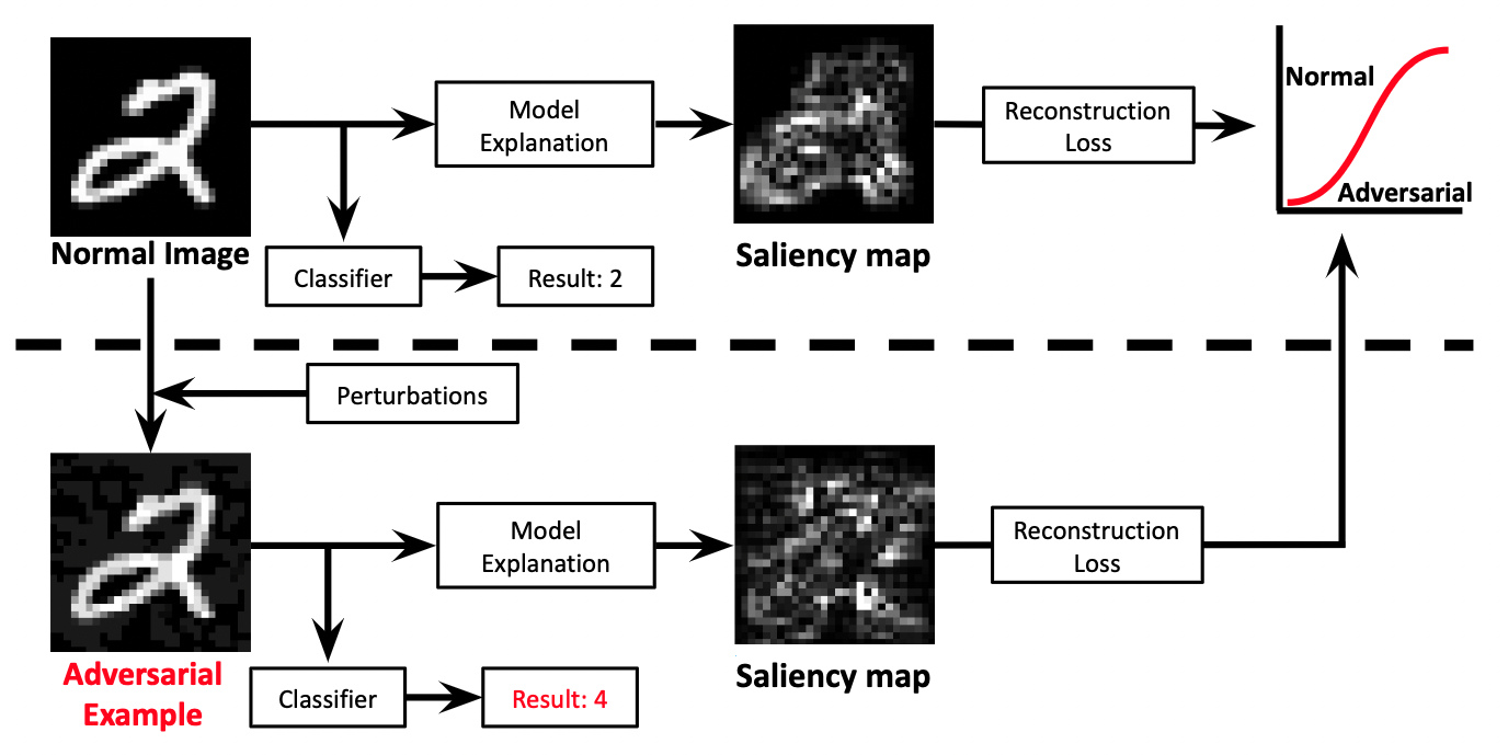
In this section, we illustrate our method: Unsupervised Detection of Adversarial Examples with Model Explanations. We first explain the threat model, and then illustrate our approach in detail. An overview of our method is illustrated in Figure 1.
3.1. Threat Model
In this paper, we consider an inspector for the given machine learning classifier , who wishes to detect (and possibly filter) whether a given input to the model is maliciously crafted to fool the decisions (i.e., the input is an adversarial example). Throughout the paper, we will refer to the model subject to attack as the target classifier.
The attacker maliciously crafts adversarial examples in order to fool the decision of the target classifier. We assume that the attacker uses state-of-the-art methods such as FGSM (Goodfellow et al., 2015), PGD (Madry et al., 2018), or MIM (Dong et al., 2018), and has access to the training and test samples, as well as the model parameters necessary to conduct the attacks.
3.2. Our Detection Method
As noted in Section 1, our method is based on the insight that adding small perterbations to generate adversarial examples could result in unusual explanations. Throughout the paper, we denote the explanation of for DNN as . We will often denote it as , when is clear from the context.
Taking advantage of this insight, our method performs unsupervised detection based on three steps: i) generating input explanations, ii) training reconstructor networks using generated explanations, and iii) utilizing reconstructor networks to separate normal and adversarial examples.
Generating input explanations.
In our proposed method, the inspector is assumed to have access to the training samples that was used to train the target classifier. In order to perform unsupervised anomaly detection based on the model explanations, the inspector first generates input explanations for the target model, using training samples.
As noted in Section 2, explanations of the target classifier depends on the output label . As the explanations are differently applied for each label, the inspector organizes generated explanations according to the corresponding input’s output label. We denote by as a set of input explanations for the inputs in the training dataset with output label .
Training reconstructor networks.
Once the explanations for training samples are collected and organized, the inspector then trains reconstructor networks — one for each class label — which reconstructs the explanations for an input with corresponding class label. Such reconstructor networks will later be used in separating adversarial examples from benign examples.
For each class label , the inspector trains a parameterized network reconstructing input explanations, solving the following optimization:
where is a reconstruction loss for network on .
Separating adversarial examples.
Lastly, the inspector utilizes the trained reconstructor networks in order to separate adversarial examples from benign examples. As the networks are optimized to reconstruct model explanations of training samples, it will show poor reconstruction quality when an unusual shape of explanation is given. Hence, when the reconstruction error is above certain threshold, it is likely that the given input is adversarially crafted.
Formally, for a given suspicious input , the inspector first obtains the class label and its explanation . If the reconstruction error of is larger than given threshold for label (i.e., ), the inspector concludes that the input is likely to be an adversarial example.
4. Evaluation
In this section, we evaluate the effectiveness of our proposed detection method.
| Original | Adversarial | |||
|---|---|---|---|---|
| FGSM | PGD | MIM | ||
| Input |
|
|
|
|
| Gradient |
|
|
|
|
| Recons. |
|
|
|
|
4.1. Experimental Setup
We evaluate our method using the MNIST handwritten digit dataset (MNIST) (LeCun et al., 1998). Using MNIST dataset, we first train the target classifier, which is subject to the adversarial attacks. In our evaluations, we trained a simple Convolutional Neural Network using the standard 60,000-10,000 train-test split of MNIST dataset. Trained target classifier had ¿99% and ¿98% classification accuracies for training and test dataset, respectively.
Given the target classifier and the training dataset, model explanations are collected to train a network reconstructing them. In our evaluations, we used input gradients (Simonyan et al., 2014) as model explanations to generate saliency maps. For each class label, the saliency maps for each MNIST training data with corresponding label is collected and used to train the reconstructor network. For all reconstructor networks, we used a simple autoencoder consisting of a single hidden layer. Summary on the model architectures can be found in Table 1.
In order to evaluate the effectiveness of our detection method, we crafted adversarial examples using all 70,000 MNIST images and filtered out unsuccessful attacks (i.e., adding perturbation does not change the original class label). For (successful) adversarial examples, saliency maps were obtained and combined with the saliency maps of the (benign) MNIST test dataset to form a evaluation dataset for our detection method. For a detailed configuration on datasets, we refer to Appendix A.
| Target classifier | Reconstructor | ||
|---|---|---|---|
| Conv.ReLU | 3 3 32 | Dense.ReLU | 784 |
| Dense.ReLU | 128 | Dense.ReLU | 64 |
| Softmax | 10 | Dense.ReLU | 784 |
| Adv. Attack | (Feinman et al., 2017) | (Lee et al., 2019) | (Liang et al., 2021) | (Ma et al., 2018) | Ours | |
|---|---|---|---|---|---|---|
| FGSM | 0.7768 | 0.7952 | 0.9514 | 0.8030 | 0.9233 | |
| 0.8672 | 0.8977 | 0.9826 | 0.7767 | 0.9573 | ||
| 0.8925 | 0.9380 | 0.9887 | 0.8681 | 0.9693 | ||
| PGD (BIM*) | 0.9419 | 0.8096 | 0.9716 | 0.8092 | 0.9839 | |
| 0.9768 | 0.8330 | 0.9890 | 0.9027 | 0.9894 | ||
| 0.9801 | 0.7088 | 0.9896 | 0.9574 | 0.9901 | ||
* BIM (Basic Iterative Method) (Kurakin et al., 2017) is a variant of FGSM, similar to PGD. As in some papers PGD is described as a specialized BIM attack, we included results of BIM attacks in the table.
4.2. Experimental Results
Effect of input perturbations on explanations.
Figure 2 shows pairs of input image (Input), explanation (Gradient) obtained from the target classifier, and the reconstruction (Recons.) from the trained reconstructor networks, for an example MNIST image and adversarial examples crafted from the image. Here, we confirm our insight that small adversarial perturbations to inputs can lead to noticeable changes in their explanations. Since the reconstructor networks are only trained on benign explanations (input explanations of benign examples), we see that reconstructions of adversarial explanations (input explanations of adversarial examples) are more noisy than the reconstruction of the explanation of original image.
Adversarial detection performance.


In order to evaluate the effectiveness of our proposed detection method, we measure Area Under the ROC Curve (AUC). As our method uses multiple reconstructor networks, we record multiple values of AUC — each corresponding to a given class label — as well as their average.
Figure 3 shows the trend of AUC values under different adversarial attack scenarios. For each attack, we plot the min, max, and average values of AUC according to the severity of attack (i.e., value of ). While our method has harder time separating adversarial examples with smaller noise level, average AUC stays relatively high even in its lowest values (¿95% for FGSM, ¿97% for PGD and MIM, when ).
Our methods show high performance (average AUC of 0.9583 for FGSM, 0.9942 for PGD, 0.9944 for MIM) in the standard adversarial attack setting of for MNIST dataset. This can be also confirmed by observing Figure 4, where the ROC curves of our detection method for different class labels are plotted.
Note that only a single set (i.e., one per class label) of reconstructor networks is used in all of the attack scenarios. The results clearly show that our defense method can generalize across multiple attack algorithms – which is impressive, considering that no single adversarial example is provided in the training phase. For a more detailed benchmark results, we refer to Appendix B.
Quantitative comparison to previous approaches.
We quantitatively compare our method’s adversarial detection accuracy to a number of previous approaches. Specifically, we compare our results with the results from four different existing works ((Feinman et al., 2017; Lee et al., 2019; Liang et al., 2021; Ma et al., 2018)), where the benchmark results are recorded in (Sutanto and Lee, 2021).
Table 2 shows comparison on adversarial detection accuracies of the proposed and existing approaches. In all experiments, our method performs the best or the second best in detecting adversarial samples. The results show that our method is comparable to, and often outperforms existing methods.
5. Conclusion
In this paper, we propose a novel methodology in detecting adversarial examples using model explanations. Our method is motivated from the insight that even when small perturbation is added to the input, model explanations can drastically be altered. Taking advantage of this, we suggested an anomaly detection of adversarial examples using a network optimized to reconstruct the model explanations from benign examples. Unlike supervised methods, our method is attack-agnostic, in that it does not require pre-generated adversarial samples.
In our experiments using MNIST handwritten dataset, we showed that our method is capable of separating benign and adversarial examples with high performance, comparable to, or better than existing approaches. We argue that our method is more efficient due to its unsupervised manner; with single training of reconstructor networks, multiple state-of-the-art attacks such as FGSM, PGD, and MIM can be prevented. To the best of our knowledge, this work is the first in suggesting unsupervised defense method using model explanations.
Acknowledgment
This work was developed with the suppport of Institute of Information & communications Technology Planning & Evaluation (IITP) grant, funded by the Korea government (MSIT) (No.2020-0-00153, Penetration Security Testing of ML Model Vulnerabilities and Defense).
References
- (1)
- Bhagoji et al. (2017) Arjun Nitin Bhagoji, Daniel Cullina, and Prateek Mittal. 2017. Dimensionality Reduction as a Defense against Evasion Attacks on Machine Learning Classifiers. CoRR abs/1704.02654 (2017).
- Dong et al. (2018) Yinpeng Dong, Fangzhou Liao, Tianyu Pang, Hang Su, Jun Zhu, Xiaolin Hu, and Jianguo Li. 2018. Boosting Adversarial Attacks With Momentum. In 2018 IEEE Conference on Computer Vision and Pattern Recognition, CVPR 2018, Salt Lake City, UT, USA, June 18-22, 2018. IEEE Computer Society, 9185–9193.
- Eykholt et al. (2018) Kevin Eykholt, Ivan Evtimov, Earlence Fernandes, Bo Li, Amir Rahmati, Chaowei Xiao, Atul Prakash, Tadayoshi Kohno, and Dawn Song. 2018. Robust Physical-World Attacks on Deep Learning Visual Classification. In CVPR. IEEE Computer Society, 1625–1634.
- Feinman et al. (2017) Reuben Feinman, Ryan R. Curtin, Saurabh Shintre, and Andrew B. Gardner. 2017. Detecting Adversarial Samples from Artifacts. CoRR abs/1703.00410 (2017).
- Fidel et al. (2020) Gil Fidel, Ron Bitton, and Asaf Shabtai. 2020. When Explainability Meets Adversarial Learning: Detecting Adversarial Examples using SHAP Signatures. In IJCNN. IEEE, 1–8.
- Gong et al. (2017) Zhitao Gong, Wenlu Wang, and Wei-Shinn Ku. 2017. Adversarial and Clean Data Are Not Twins. CoRR abs/1704.04960 (2017).
- Goodfellow et al. (2015) Ian J. Goodfellow, Jonathon Shlens, and Christian Szegedy. 2015. Explaining and Harnessing Adversarial Examples. In ICLR (Poster).
- Grosse et al. (2017) Kathrin Grosse, Praveen Manoharan, Nicolas Papernot, Michael Backes, and Patrick D. McDaniel. 2017. On the (Statistical) Detection of Adversarial Examples. CoRR abs/1702.06280 (2017).
- Kurakin et al. (2017) Alexey Kurakin, Ian J. Goodfellow, and Samy Bengio. 2017. Adversarial examples in the physical world. In 5th International Conference on Learning Representations, ICLR 2017, Toulon, France, April 24-26, 2017, Workshop Track Proceedings. OpenReview.net.
- LeCun et al. (1998) Yann LeCun, Léon Bottou, Yoshua Bengio, and Patrick Haffner. 1998. Gradient-Based Learning Applied to Document Recognition. In Proceedings of the IEEE, Vol. 86. 2278–2324.
- Lee et al. (2019) Sangheon Lee, Noo-Ri Kim, YoungWha Cho, Jae-Young Choi, Suntae Kim, Jeong-Ah Kim, and Jee-Hyong Lee. 2019. Adversarial Detection with Gaussian Process Regression-based Detector. KSII Trans. Internet Inf. Syst. 13, 8 (2019), 4285–4299.
- Li and Li (2017) Xin Li and Fuxin Li. 2017. Adversarial Examples Detection in Deep Networks with Convolutional Filter Statistics. In ICCV. IEEE Computer Society, 5775–5783.
- Liang et al. (2021) Bin Liang, Hongcheng Li, Miaoqiang Su, Xirong Li, Wenchang Shi, and Xiaofeng Wang. 2021. Detecting Adversarial Image Examples in Deep Neural Networks with Adaptive Noise Reduction. IEEE Trans. Dependable Secur. Comput. 18, 1 (2021), 72–85.
- Lundberg and Lee (2017) Scott M. Lundberg and Su-In Lee. 2017. A Unified Approach to Interpreting Model Predictions. In NIPS. 4765–4774.
- Ma et al. (2018) Xingjun Ma, Bo Li, Yisen Wang, Sarah M. Erfani, Sudanthi N. R. Wijewickrema, Grant Schoenebeck, Dawn Song, Michael E. Houle, and James Bailey. 2018. Characterizing Adversarial Subspaces Using Local Intrinsic Dimensionality. In ICLR. OpenReview.net.
- Madry et al. (2018) Aleksander Madry, Aleksandar Makelov, Ludwig Schmidt, Dimitris Tsipras, and Adrian Vladu. 2018. Towards Deep Learning Models Resistant to Adversarial Attacks. In 6th International Conference on Learning Representations, ICLR 2018, Vancouver, BC, Canada, April 30 - May 3, 2018, Conference Track Proceedings. OpenReview.net.
- Metzen et al. (2017) Jan Hendrik Metzen, Tim Genewein, Volker Fischer, and Bastian Bischoff. 2017. On Detecting Adversarial Perturbations. In ICLR (Poster). OpenReview.net.
- Nesti et al. (2021) Federico Nesti, Alessandro Biondi, and Giorgio C. Buttazzo. 2021. Detecting Adversarial Examples by Input Transformations, Defense Perturbations, and Voting. CoRR abs/2101.11466 (2021).
- Pang et al. (2018) Tianyu Pang, Chao Du, Yinpeng Dong, and Jun Zhu. 2018. Towards Robust Detection of Adversarial Examples. In NeurIPS. 4584–4594.
- Simonyan et al. (2014) Karen Simonyan, Andrea Vedaldi, and Andrew Zisserman. 2014. Deep Inside Convolutional Networks: Visualising Image Classification Models and Saliency Maps. In ICLR (Workshop Poster).
- Sutanto and Lee (2021) Richard Evan Sutanto and Sukho Lee. 2021. Real-Time Adversarial Attack Detection with Deep Image Prior Initialized as a High-Level Representation Based Blurring Network. Electronics 10, 1 (2021).
- Szegedy et al. (2014) Christian Szegedy, Wojciech Zaremba, Ilya Sutskever, Joan Bruna, Dumitru Erhan, Ian J. Goodfellow, and Rob Fergus. 2014. Intriguing properties of neural networks. In ICLR (Poster).
- Tian et al. (2018) Shixin Tian, Guolei Yang, and Ying Cai. 2018. Detecting Adversarial Examples Through Image Transformation. In AAAI. AAAI Press, 4139–4146.
Appendix A Datasets for Reconstructor Networks
| Adv. Attack | Training | Test | ||
|---|---|---|---|---|
| normal | normal | adversarial | ||
| FGSM | 60000* | 10000** | 5797 | |
| 22649 | ||||
| 39524 | ||||
| 51191 | ||||
| 57272 | ||||
| 60287 | ||||
| PGD | 60000* | 10000** | 8671 | |
| 55432 | ||||
| 69604 | ||||
| 69818 | ||||
| 69823 | ||||
| 69823 | ||||
| MIM | 60000* | 10000** | 8679 | |
| 53150 | ||||
| 69402 | ||||
| 69822 | ||||
| 69823 | ||||
| 69825 | ||||
* saliency maps of MNIST training images
** saliency maps of MNIST test images
Appendix B Detailed Performance Benchmark
| Adv. Attack | Accuracy | F1 Score | Avg. AUC | |
|---|---|---|---|---|
| FGSM | 0.8772 | 0.7680 | 0.9299 | |
| 0.9233 | 0.9230 | 0.9583 | ||
| 0.9470 | 0.9543 | 0.9690 | ||
| 0.9573 | 0.9643 | 0.9733 | ||
| 0.9644 | 0.9725 | 0.9775 | ||
| 0.9693 | 0.9747 | 0.9813 | ||
| PGD | 0.9301 | 0.8898 | 0.9723 | |
| 0.9839 | 0.9848 | 0.9942 | ||
| 0.9884 | 0.9896 | 0.9960 | ||
| 0.9894 | 0.9909 | 0.9961 | ||
| 0.9898 | 0.9908 | 0.9962 | ||
| 0.9901 | 0.9912 | 0.9963 | ||
| MIM | 0.9416 | 0.9096 | 0.9799 | |
| 0.9839 | 0.9852 | 0.9944 | ||
| 0.9882 | 0.9899 | 0.9959 | ||
| 0.9897 | 0.9910 | 0.9960 | ||
| 0.9902 | 0.9915 | 0.9961 | ||
| 0.9910 | 0.9924 | 0.9965 | ||