Universal tripartite entanglement in one-dimensional many-body systems

Quantum entanglement has come to play a key role in our understanding of emergent phenomena in quantum many-body physics and modern numerical methods. Most attention has focused on bipartite entanglement, e.g. properties of a pure state on two parties $\ket{\psi}_{AB}$. The entanglement entropy $S(A)$ is the unique measure of bipartite entanglement because, up to reversible local operations and classical communication, the EPR pair is the unique form of bipartite entanglement. In contrast, a pure tripartite state $\ket{\psi}_{ABC}$ admits a large (presumably infinite) number of distinct forms of entanglement, and consequently a variety of tripartite entanglement measures have been proposed [1]. But it remains relatively unexplored what universal features such measures might reveal about a many-body system [2, 3, 4, 5, 6, 7, 8, 9].

Recently two tripartite entanglement measures, the entanglement of purification $E_{P}(A:B)$ [10] and the “reflected entropy” $S_{R}(A:B)$ [11] have been applied to many-body physics within the context of holographic duality. As motivation, recall that the Ryu-Takayanagi formula equates the bipartite entanglement entropy of a boundary theory to the area of a minimal surface in its holographic dual [12], a central result in the effort to relate the emergence of spacetime geometry to quantum entanglement. It is then natural ask whether there are multi-partite entanglement measures which might also have a dual geometric interpretation. In Refs. [13, 14] it was conjectured that the minimal cross section of the bulk “entanglement wedge” joining two parties, $E_{W}(A:B)$, is dual to the entanglement of purification in the boundary, $E_{P}=E_{W}$. More recently, however, by developing a field-theoretic method for calculating $S_{R}$ in generic conformal field theories (CFTs), it was shown that $S_{R}=2E_{W}$ [11]. In general $S_{R}\neq 2E_{P}$, so one possible resolution is that their equality is a special property of holographic CFTs which is violated at subleading order in large-$N$ expansion ¹¹1It has also been argued that the logarithmic negativity is dual to $E_{W}$ [7], but $\mathcal{E}_{N}$ is not lower bounded by $I$, so we do not consider it here.. The gap between them, $2E_{P}-S_{R}$, would then constitute an interesting entanglement measure of this violation. But investigating this discrepancy requires a method for computing these quantities in generic many-body systems.

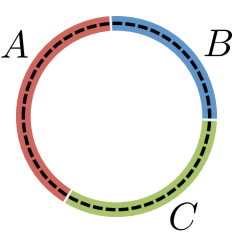
In this work we derive a method for computing $E_{P}$ and $S_{R}$ in 1D lattice models. To summarize our findings it is convenient to define UV-regularized version of these quantities ²²2$2E_{P}(A:B),S_{R}(A:B)$ and $I(A:B)$ all scale logarithmically with the UV cutoff with the same coefficient $c/3$ in front, see Ref. 13, 14, 11., $g(A:B)\equiv 2E_{P}(A:B)-I(A:B)\geq 0$ and $h(A:B)\equiv S_{R}(A:B)-I(A:B)\geq 0$, where $I$ is the mutual information ³³3Note that while the constituents are, $g,h$ are not monotonic under quantum operations on $A,B$.. For the tripartition of a ring shown in Fig. 1, holographic duality predicts that they take on the universal value $g=h=\frac{c}{3}\log(2)$, where $c$ is the central charge of the CFT ⁴⁴4In this computation, the regions $A,B$ are taken to touch and the UV divergences in $E_{W},I$ are regulated by a radial cutoff which is taken to zero after the subtraction $2E_{W}-I$ [14]. This prescription corresponds to the lattice regularization employed in our numerical results. An alternative procedure, in which the quantities are regularized by a small spacing between $A,B$, yields a different result [13].. But what about in a generic lattice model? As a limiting case, we start by proving structure theorems for states with $g,h=0$ which imply that $h=0$ if an only if a state is gapped ($c=0$), while $g=0$ if and only if the system is gapped and does not spontaneously break a symmetry. We then develop a method for numerically computing $g,h$ from a lattice Hamiltonian on systems up to $N\sim 100$ sites. As expected, we find that $h=\frac{c}{3}\log 2$ is universal. However we find that $g\geq h$ and depends on the operator content of the CFT in addition $c$, yet is nevertheless completely universal. Thus $2E_{P}-S_{R}=g-h$ constitutes a new and universal tripartite entanglement invariant of CFTs.

$E_{P}$ and $S_{R}$ — We first review the definitions of the entanglement of purification $E_{P}(A:B)$ and reflected entropy $S_{R}(A:B)$. Unlike the bipartite entanglement entropy, which is a function of a reduced density matrix on one party, these mixed state entanglement measures are functions of the reduced density matrix on two parties, $\rho_{AB}$, or equivalently its purification $\ket{\psi}_{ABC}$, where $\rho_{AB}=\operatorname{Tr}_{C}\ket{\psi}\bra{\psi}$.

The entanglement of purification $E_{P}(A:B)$ [10] is the minimum of the entanglement entropy $S_{AC_{L}}$ over all purifications $\ket{\phi}_{ABC_{L}C_{R}}$ of $\rho_{AB}$ to another pair of systems $C=C_{L}C_{R}$:

The partitions of the subsystems are depicted schematically in Fig. 1. In principle the auxiliary space $C_{L}C_{R}$ can be arbitrary, but the minimal $S_{AC_{L}}$ can always be achieved with $\dim(\mathcal{H}_{C_{L}}),\,\dim(\mathcal{H}_{C_{R}})\leq\operatorname{rank}(\rho_{AB})$.[19] We may alternatively rephrase Eq. (1) as a minimization over unitary operations $U_{C}$ restricted to $C_{L}C_{R}$ starting from an arbitrary purification $\ket{\phi_{0}}_{ABC_{L}C_{R}}$ of sufficiently large dimension,

which is the viewpoint taken in our numerical approach.

$E_{P}$ is lower bounded by the mutual information [10], $E_{P}(A:B)\geq I(A:B)/2$, so we define a non-negative quantity

The physical intuition behind this new quantity is that the subtraction of the mutual information removes correlations which are purely bipartite, as will be made more precise by the structure theorems below.

To define the reflected entropy $S_{R}(A:B)$, we instead pick a particular purification of $\rho_{AB}$ known as the canonical purification $\ket{\sqrt{\rho_{AB}}}$. It is defined as follows: we first take the unique non-negative square root of the reduced density matrix $\rho_{AB}$, and then regard the operator $\sqrt{\rho_{AB}}$ as a state $\ket{\sqrt{\rho_{AB}}}\in\mathcal{H}_{A}\otimes\mathcal{H}_{B}\otimes\mathcal{H}^{*}_{A}\otimes\mathcal{H}^{*}_{B}$. The reflected entropy $S_{R}(A:B)$ is defined as

It is shown in Ref. 11 that $S_{R}(A:B)\geq I(A:B)$, so we define the nonnegative quantity

In order to interpret the nature of the tripartite entanglement captured by these quantities, we derive “structure theorems” for states which saturate these lower bounds, i.e., states with $g=0$ or $h=0$.

States with $g(A:B)=0$ — We first define a class of pure tripartite wavefunctions known as triangle states.

In other words, a triangle state can be obtained by pair-wise distributing bipartite-entangled states followed by local unitaries. In this sense, a triangle state lacks nontrivial tripartite entanglement. We prove the following theorem in the Supplemental Material (SM) [20, 21].

The “only if” direction can be shown by noting that $2E_{P}(A:B)=I(A:B)$ in the purification $\ket{\psi}_{ABC}$ of $\rho_{AB}$. The proof of the “if” direction is more complicated, and is presented in SM [20].

Conversely, $g(A:B)>0$ implies that $\ket{\psi}_{ABC}$ contains tripartite entanglement that cannot be factorized pairwise. For example, for a GHZ state $\ket{\psi}_{ABC}=\sqrt{d^{-1}}\sum_{j=1}^{d}\ket{j_{A}j_{B}j_{C}}$ the optimal purification of $\rho_{AB}$ is $\ket{\psi}_{ABC}$ itself [14], resulting in $g(A:B)=\log d$. It can also be shown that the $W$ state has nonzero $g(A:B)$. This is in accordance with the fact the GHZ state and $W$ state are not triangle states [22].

States with $h(A:B)=0$ — It can be verified that a triangle state has $h(A:B)=0$, so $h(A:B)\neq 0$ also implies irreducible tripartite entanglement. But for the GHZ state, $g(A:B)\neq 0$ while $h(A:B)=0$, which suggests that that some forms of tripartite entanglement are “invisible” to $h$.

To make this precise we introduce the notion of sum of triangle states.

For example, the GHZ state is a SOTS with $p_{j}=\frac{1}{d}$ and the triangle state is a SOTS for which $p_{j}=1$ for exactly one $j$. By using the structure theorem for states satisfying strong subadditivity [23], we prove [20] the following:

As a corollary, while in general $h(A:B)\neq h(B:C)\neq h(C:A)$, if one vanishes then all of them vanish (and likewise for $g$).

$g$ and $h$ for 1D gapped systems — We now give a physical interpretation of these structure theorems in the context of 1D Hamiltonians: we argue that on a ring with the tripartition shown in Fig. 1, a system is gapped if and only if $h=0$, and gapped without long-range order if and only if $g=0$. As motivation, consider the two limiting gapped phases of the 1D Ising model: the symmetric paramagnet, $\ket{\mathrm{PM}}=\ket{\rightarrow\rightarrow\cdots}$, and the ferromagnet $\ket{\mathrm{FM}}=\frac{1}{\sqrt{2}}\big{(}\ket{\mathord{\uparrow\uparrow}\cdots}+\ket{\mathord{\downarrow\downarrow}\cdots}\big{)}$. When partitioned into 3 subsystems, the $\ket{\mathrm{PM}}$ ($\ket{\mathrm{FM}}$) state corresponds to a product state (GHZ state), so it will have $g=0$ ($g=\log 2$) and for both, $h=0$. Indeed, we see that $g$ is sensitive to the “cat state” structure of the exact ground state in a symmetry-broken phase, so will generically detect the multiplicity of super-selection sectors. Away from these extremal points, the ground state develops additional short-range entanglement. However, so long as sizes of the regions $N_{A},N_{B},N_{C}$ are larger than the correlation length $\xi$, this additional entanglement simply dresses the product state within each superselection sector into a triangle state, and so with exponential accuracy in $N/\xi$, $g$ and $h$ are unchanged.

The argument can be phrased most precisely in the language of matrix product states. We first take a finite-dimensional MPS as an approximation to the ground state of a 1D system ⁵⁵5There is a caveat to use the finite-dimensional MPS as an approximation. It is only rigorously proven that the state can be faithfully represented if bond dimension grows with the system size [37, 38]. For a finite bond dimension, it has only been shown that local properties can be well approximated [39]. In order to make our argument, we have to assume that the finite bond dimension does not result in a substantial error in $g$ or $h$, which are nonlocal properties of the ground state. Despite not rigorous proven, the assumption is highly plausible because of empirical success of infinite MPS algorithms, where correlation functions and entanglement properties at long distances are extracted from a finite-dimensional MPS. Therefore the argument could be regarded as heuristic for a general gapped theory. However, it is rigorous if the ground state can be exactly represented by a finite-dimensional MPS, for example that of a MPS parent Hamiltonian [29].. The thermodynamic limit is taken by fixing $N_{A}/N,N_{B}/N$ and taking $N\rightarrow\infty$, where $N$ is the total system size. In the thermodynamic limit we can then apply the standard MPS coarse-graining procedure [25] to obtain a fixed-point MPS. If the initial correlation length is finite [26], the state flows to an MPS with $\xi=0$. It is straightforward to show that a $\xi=0$ MPS is precisely the $N$-party generalization ⁶⁶6The generalization of a triangle state to many parties is a polygon state, which is discussed in detail in [20]. A polygon state is a triangle state with respect to any tripartition into contiguous regions. of a triangle state [25, 28], so by the structure theorems we obtain $g=h=0$. On the other hand, if the MPS has an infinite correlation length (e.g., it is a cat state as occurs for spontaneous symmetry breaking or phase coexistence), then it flows to a sum of $\xi=0$ MPS which are locally orthogonal [29, 20]. Thus in the long-range ordered phase we have $g\neq 0$ and $h=0$. These cases are analyzed in greater detail in [20]. Note that the precise statement of our claim is thus as follows: A fixed-point MPS has $h(A:B)=0$ for all contiguous tripartitions. Since all MPS flow towards fixed-point MPS under coarse graining, $h(A:B)\to 0$ as $N_{A},N_{B}\to\infty$ ⁷⁷7Technically, taking the limit assumes the continuity of $g(A:B)$ and $h(A:B)$ with respect to the reduced density matrix $\rho_{AB}$ [20]. The continuity property of $E_{P}$ and $S_{R}$ has already been proven in [10, 40]..

Gapless systems — At a critical point $g$ and $h$ need not vanish. In fact, they are universal constants which depend only on the emergent CFT in the thermodynamic limit.

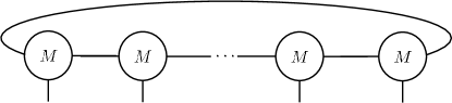
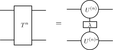
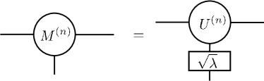
We now briefly describe the algorithm to compute $g$ and $h$ of the ground state of a critical quantum spin chain with $N$ sites and Hamiltonian $H$. First the ground state $\ket{\psi}_{ABC}$ is obtained in the form of a periodic uniform MPS (puMPS) [31, 32, 33]. A puMPS consists of $N$ copies of the same rank-3 tensor $M$ with dimensions $D\times D\times d$, where $d$ is the dimension of the Hilbert space on each site, and $D$ is the bond dimension which grows polynomially with the system size $N$ (Fig. 2). The tensor $M$ is obtained variationally by minimizing the expectation value of $H$. We then apply the standard MPS coarse-graining procedure [25, 20] to “compress” the Hilbert space of each region down to a smaller one via a sequence of isometries, $\mathcal{H}_{\alpha}\to\mathcal{H}_{\tilde{\alpha}}$. Because the entropy of each region is sub-extensive, $S_{\alpha}\ll N_{\alpha}\log(d)$ – even at a critical point – we can reduce the dimension of the Hilbert space $\tilde{d}_{\alpha}\ll d_{\alpha}$ while preserving all the bipartite and tripartite entanglement properties among the three parties $A$, $B$ and $C$ to high-accuracy. The coarse-grained state $\ket{\tilde{\psi}}_{\tilde{A}\tilde{B}\tilde{C}}$ can be represented by a MPS with three tensors $M_{\alpha}$ with dimensions $D\times D\times\tilde{d}_{\alpha}$ (Fig. 2), where $\tilde{d}_{\alpha}\leq D^{2}$. $D,\tilde{d}_{\alpha}$ grow polynomial with system size; as an example, for the Ising CFT we use $D=12$, $\tilde{d}_{\alpha}=36$ for $N=24$ and $D=26$, $\tilde{d}_{\alpha}=100$ for $N=84$.

We compute $S_{R}(A:B)$ according to Eq. (4) in the dense representation. Assuming that $\tilde{d}_{A}\leq\tilde{d}_{B}$, the total time cost scales as $\mathcal{O}\big{(}\tilde{d}^{4}_{A}\tilde{d}^{2}_{B}\big{)}$. To compute $E_{P}(A:B)$, we first make a random split of $\mathcal{H}_{\tilde{C}}$ into $\mathcal{H}_{\tilde{C}_{L}}\otimes\mathcal{H}_{\tilde{C}_{R}}$ with dimensions $\tilde{d}_{C_{L}}\times\tilde{d}_{C_{R}}$. We then numerically minimize the entanglement entropy of $\tilde{A}\tilde{C}_{L}$ with respect to a unitary $U_{\tilde{C}}$ on $\tilde{C}$,

We verified numerically that the $\tilde{d}_{\alpha}$ are large enough to achieve the (near) optimal purification. The numerical optimization can be performed with, e.g., the non-linear conjugate gradient algorithm, since the gradient can be constructed explicitly (see [20]). The time cost of each gradient calculation scales as $\mathcal{O}(\tilde{d}^{2}_{A}\tilde{d}_{B}\tilde{d}^{2}_{C})$, assuming that $\tilde{d}_{A}\leq\tilde{d}_{B}$. The mutual information $I(A:B)$ can also be computed using the coarse-grained state, with time cost $O(\tilde{d}^{3}_{\max})$, where $\tilde{d}_{\max}\equiv\max_{\alpha}\{\tilde{d}_{\alpha}\}$.

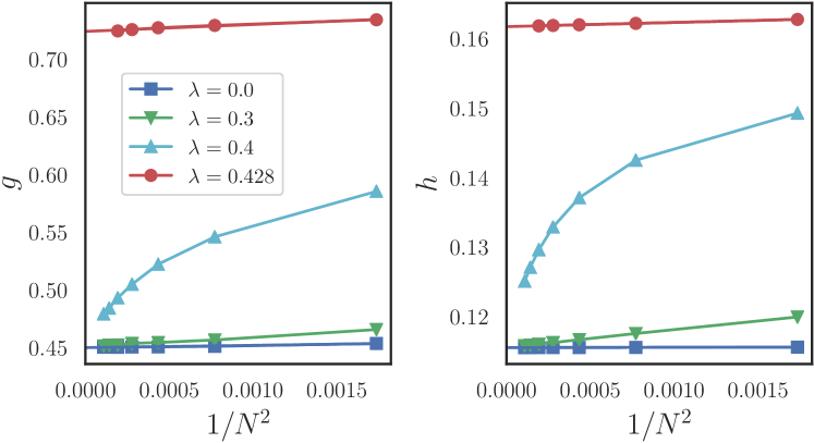
$g$ and $h$ for various CFTs — In order to show that $g$ and $h$ are universal, we study the Ising model with an irrelevant near-to-nearest neighbor interaction [34],

where $X_{j}$($Z_{j}$) are Pauli $X$($Z$) matrices on sites $j$ and periodic boundary conditions are assumed. The model is critical described by the Ising CFT for $\lambda<\lambda^{*}$, gapped for $\lambda>\lambda^{*}$, where the transition at $\lambda^{*}\approx 0.428$ is described by the tricritical Ising CFT [34]. We study four parameter values, $\lambda=0,0.3,0.4,\lambda^{*}$, where the first three correspond to the Ising CFT and the last correspond to the tricritical Ising CFT.

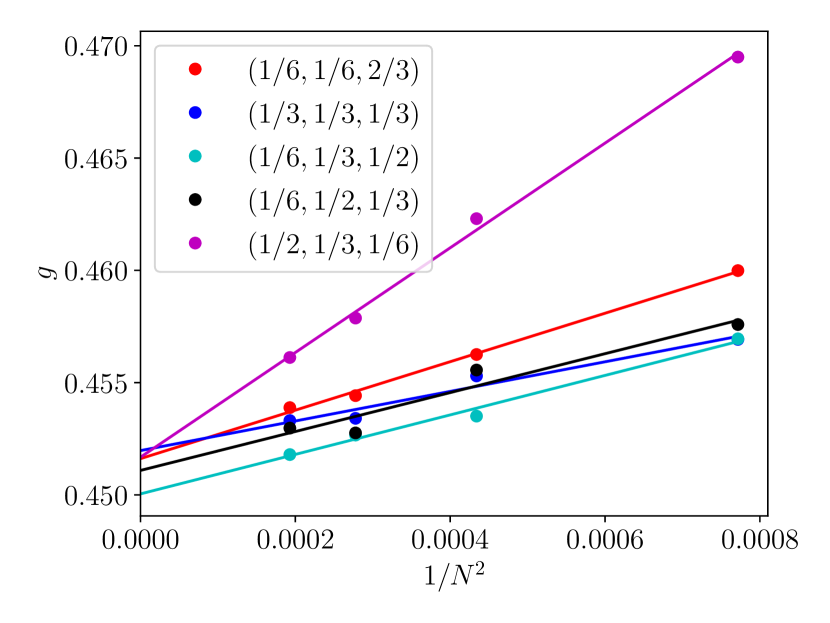
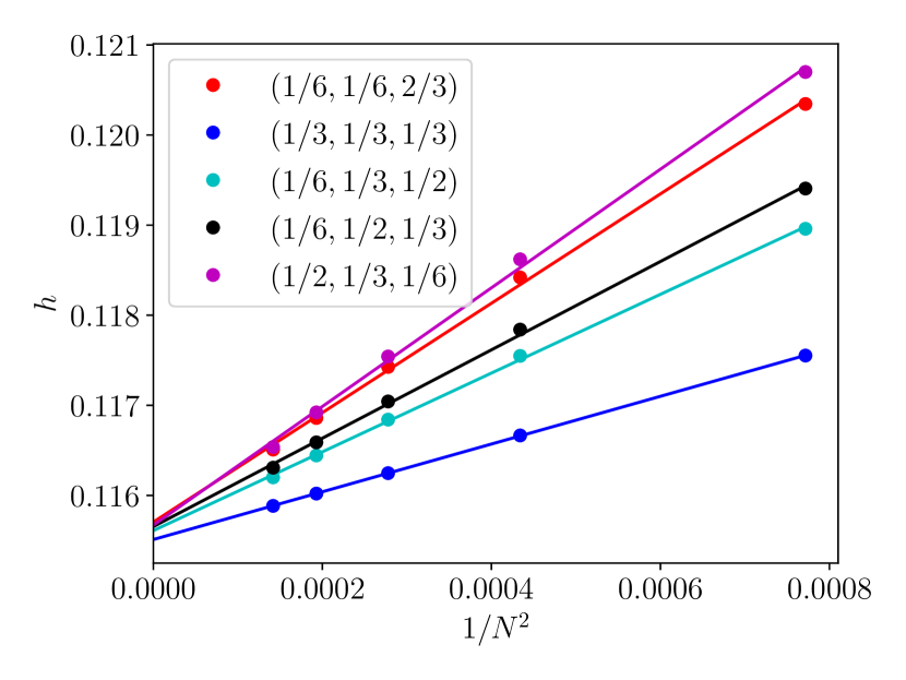
We fix $N_{A}=N_{B}=N_{C}=N/3$ and compute $g(A:B)$ and $h(A:B)$ as a function of $N$, shown in Fig. 3. We see that both $g$ and $h$ converge to a constant as $N\rightarrow\infty$ ⁸⁸8The extrapolation is based on the numerical observation that $g$ and $h$ converges as a power of $1/N$, where the power is determined empirically.. Furthermore, the constant is the same for $\lambda=0$ and $\lambda=0.3$, indicating that $g$ and $h$ are universal. We denote the universal quantities as $g^{{\textsl{\tiny CFT}}}$ and $h^{{\textsl{\tiny CFT}}}$. At $\lambda=\lambda^{*}\approx 0.428$, we obtain a different value that corresponds to the tricritical Ising CFT. At $\lambda=0.4$, both $g$ and $h$ go through a renormalization group flow from the tricritical Ising CFT to the Ising CFT, analogous to the spectral flow observed in Ref. 31. The values of $g^{{\textsl{\tiny CFT}}}$ and $h^{{\textsl{\tiny CFT}}}$ for various CFTs are summarized in Table 1.

We also verified that the values of $g^{{\textsl{\tiny CFT}}}$ and $h^{{\textsl{\tiny CFT}}}$ do not depend on the relative sizes of $A,B,C$ [20]. For any ratio $N_{A}/N$ and $N_{B}/N$, once we take the thermodynamic limit $N\rightarrow\infty$, both $g(A:B)$ and $h(A:B)$ converge to the universal constants $g^{{\textsl{\tiny CFT}}}$ and $h^{{\textsl{\tiny CFT}}}$.

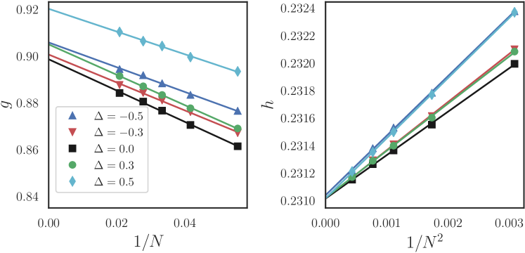
We proceed to examine how $g^{\textsl{\tiny CFT}}$ and $h^{\textsl{\tiny CFT}}$ depend on the conformal data of the CFT. To do so we compute $g^{\textsl{\tiny CFT}}$ and $h^{\textsl{\tiny CFT}}$ for the free compactified boson CFT for differing compactification radius $R$. All have the same central charge $c=1$, but the operator content depends on $R$. A concrete lattice realization of the CFT is the XXZ model,

where $-1\leq\Delta<1$ is a parameter that determines the compactification radius $R=\sqrt{2\pi/\cos^{-1}(-\Delta)}$. We compute $g^{{\textsl{\tiny CFT}}}$ and $h^{{\textsl{\tiny CFT}}}$ for different $R$’s by extrapolating $g(A:B)$ and $h(A:B)$ for different $\Delta$’s to the thermodynamic limit. The result is shown in Fig. 4 and Tab. 1, where $R=\sqrt{3},2,\sqrt{6}$ correspond to $\Delta=0.5,0,-0.5$, respectively ⁹⁹9Note that at $\Delta=0$ both $g^{{\textsl{\tiny CFT}}}$ and $h^{{\textsl{\tiny CFT}}}$ equal twice of that for the Ising CFT, in accordance with the duality between the CFTs..

We see that $h^{{\textsl{\tiny CFT}}}$ does not depend on $\Delta$ and is compatible with $h^{\textsl{\tiny CFT}}=\frac{c}{3}\log 2$. On the other hand, $g^{{\textsl{\tiny CFT}}}$ depends on $\Delta$ and thus on $R$. For example, as shown in Table I, $g^{\textsl{\tiny CFT}}$ takes on three different values at $\Delta=0,0.5,-0.5$, which correspond to $R=2,\sqrt{3},\sqrt{6}$, respectively. We conclude that $h^{{\textsl{\tiny CFT}}}$ only depends on the central charge but $g^{{\textsl{\tiny CFT}}}$ depends on the whole operator content. This feature of $h^{{\textsl{\tiny CFT}}}$ can be understood as follows. The canonical purification of $\rho_{AB}$ can be regarded as the ground state of a CFT living on a circle, divided into four contiguous segments $A,B,\bar{B},\bar{A}$. The measure $h(A:B)=S_{A\bar{A}}-S_{A}-S_{B}+S_{AB}$ involves only contiguous pieces and is hence proportional to the central charge.

Discussion — In this work we have introduced two positive quantities $g$ and $h$ which quantify the obstruction to factorizing a tripartite state into pairwise correlations. While the entanglement wedge cross section duality $E_{W}=E_{P}=S_{R}/2$ predicts $h=g=\frac{c}{3}\log(2)$, for low-$c$ CFTs like the Ising model we find $g>h=\frac{c}{3}\log(2)$. The gap $g-h$ is universal, but it remains an open question how to compute it from the underlying data of the CFT. It is natural to conjecture a general bound $g\geq h$, which would follow from the monotonicity of $S_{R}$ under a partial trace.