Universal quantum computation based on nanoscale skyrmion helicity qubits in frustrated magnets

Introduction. The skyrmion is a classical topological soliton in a continuum theory. The magnetic skyrmion has attracted tremendous attention Nagaosa_NNANO2013 ; Mochizuki_Review ; Finocchio_JPD2016 ; Wiesendanger_Review2016 ; Fert_NATREVMAT2017 ; Zhang_JPCM2020 ; Gobel_PP2021 ; Reichhardt_2021 ; Zhou_NSR2018 ; Li_MH2021 ; Tokura_CR2021 ; Yu_JMMM2021 ; Marrows_APL2021 because it may be used for building spintronic applications Nagaosa_NNANO2013 ; Mochizuki_Review ; Finocchio_JPD2016 ; Wiesendanger_Review2016 ; Fert_NATREVMAT2017 ; Zhang_JPCM2020 ; Gobel_PP2021 ; Reichhardt_2021 ; Zhou_NSR2018 ; Li_MH2021 ; Tokura_CR2021 ; Yu_JMMM2021 ; Marrows_APL2021 such as racetrack memory and logic gates Sampaio_NN2013 ; Tomasello_SREP2014 ; Xichao_SREP2015B . It is a two-dimensional swirling spin texture in thin films. There is the helicity degree of freedom associated with the direction of the swirling in frustrated magnets. The energy of skyrmions are degenerate with respect to the helicity degree of freedom without the magnetic dipole-dipole interaction (DDI) Leonov_NCOMMS2015 ; Lin_PRB2016A ; Batista_2016 ; Diep_Entropy2019 ; Xichao_NCOMMS2017 . However, the helicity is locked to two-fold degenerate Bloch-type skyrmions in the presence of the DDI Xichao_NCOMMS2017 ; Kurumaji_SCIENCE2019 . We note that skyrmions in frustrated magnets with certain perpendicular magnetic anisotropy could be stabilized without applying an external magnetic field Xia_APL2020 ; Xichao_NCOMMS2017 .

Although the skyrmion was initially introduced as a classical object, it must be a quantum object if the radius of the skyrmion is of the order of nanometer Psa ; Lohani ; Siegl ; Haller ; Maeland . Actually, nanoscale skyrmions with atomic scale have been already experimentally manufactured Heinze_NPhys2011 ; Schlenhoff ; Molina ; Grenz ; Swain ; Bruning . Most recently, it was proposed that a frustrated skyrmion can be used as a qubit Psa by quantizing its helicity.

Quantum computations are expected to be the next-generation computations Feynman ; DiVi ; Nielsen . It is realized in various systems including superconductors Nakamura , photonic systems Knill , quantum dots Loss , trapped ions Cirac , and nuclear magnetic resonance Vander ; Kane . Universal quantum computations are necessary for executing arbitrary quantum algorithm. The Solovay-Kitaev theorem dictates that only three quantum gates are enough for universal quantum computations Deutsch ; Dawson ; Universal . They are the $\pi/4$ phase shift gate, the Hadamard gate, and the controlled-NOT (CNOT) gate, where the former two operators are one-qubit operators and the latter one is a two-qubit operator. In principle, one can construct arbitrary rotation of the Bloch sphere based on these three quantum gates.

In this paper, we make the use of the two helicity states of a Bloch-type nanoscale skyrmion in frustrated magnets, where a linear combination of these two states is realized as a quantum-mechanical state. Then, we show that universal quantum computations are possible based on nanoscale skyrmion qubits by explicitly constructing the three necessary quantum gates. Our key observation is that the interlayer coupling between two skyrmions produces the Ising interaction. It is a basis of the CNOT gate. All qubit operations are executed by temporally controlling the electric field and the spin current. It is a merit of the present mechanism that an external magnetic field is not necessary. Our results may open a way toward universal quantum computations based on nanoscale skyrmions.

Classical skyrmion in frustrated magnets. A skyrmion is a centrosymmetric swirling structure of spins, whose collective coordinates are the skyrmion center and the helicity $\eta$ with $0\leq\eta<2\pi$. The spin texture located at the coordinate center is parametrized as

$$\mathbf{m}\left(x,y\right)=(\sin\theta(r)\cos\phi,\sin\theta(r)\sin\phi,\cos\theta(e)),$$

(1)

with

$$\phi=\varphi+\eta+\pi/2,$$

(2)

where $\varphi$ is the azimuthal angle ($0\leq\varphi<2\pi$) satisyfing $x=r\cos\varphi$, $y=r\sin\varphi$. We note that there is a difference from the conventional definition in Eq. (2) by the angle $\pi/2$.

There is a magnetic DDI in frustrated magnet. We have performed Xichao_NCOMMS2017 a numerical analysis of the energy of a skyrmion parametrized by Eq. (1), and found that it depends on the helicity $\eta$ as described by the effective Hamiltonian

$$H_{V}=-V\cos 2\eta,$$

(3)

where $V$ denotes a certain positive constant depending on the magnitude of the DDI.

The helicity of a classical skyrmion is locked therefore at $\eta=0$ or $\pi$, as shown in Fig. 1(a). It is used as a classical bit $(\left|0\right\rangle,\left|1\right\rangle)$ corresponding to a pair of $\eta=0$ and $\pi$, respectively.

When we apply a spin current, a helicity rotation occurs from $(\left|0\right\rangle,\left|1\right\rangle)$ to $(\left|1\right\rangle,\left|0\right\rangle)$. The effect is written in terms of the Pauli operator acting on the qubit basis

	$\displaystyle H_{J_{\text{current}}}$	$\displaystyle=$	$\displaystyle-\alpha_{J}J_{\text{current}}\left(\left|1\right\rangle\left\langle 0\right|+\left|0\right\rangle\left\langle 1\right|\right)$		(4)
		$\displaystyle=$	$\displaystyle-\alpha_{J}J_{\text{current}}\sigma_{x},$

where $\alpha_{J}$ is a constant.

On the other hand, a noncollinear spin texture induces the electric dipole Katsura ,

$$\mathbf{P}_{ij}=-\mathbf{e}_{ij}\times\left(\mathbf{S}_{i}\times\mathbf{S}_{j}\right),$$

(5)

where $i$ and $j$ are the site indices, $\mathbf{S}_{i}$ is the spin at the site $i$, $\mathbf{P}_{ij}$ is the electric dipole and $\mathbf{e}_{ij}$ is the unit vector pointing from the site $i$ to the site $j$. The total electric polarization is given by the sum of the local electric dipole $\mathbf{P}=\sum_{\left\{i,j\right\}}\mathbf{P}_{ij}$. It is coupled to the electric field $\mathbf{E}$, where the Hamiltonian is given by $\mathbf{E}\cdot\mathbf{P}$. With the use of the skyrmion configuration (1) for $\mathbf{S}_{i}$, this is numerically estimated as YaoNJP

$$H_{E_{z}}=\mathbf{E}\cdot\mathbf{P}=\alpha_{E}E_{z}\cos\eta$$

(6)

in a perpendicular electric field $\mathbf{E}=\left(0,0,E_{z}\right)$, where $\alpha_{E}$ is a constant. This is rewritten as

$$H_{E_{z}}=\alpha_{E}E_{z}\sigma_{z},$$

(7)

because $\sigma_{z}(\left|0\right\rangle,\left|1\right\rangle)^{t}=(\left|0\right\rangle,-\left|1\right\rangle)^{t}$.

Helicity qubit. When the size of a skyrmion is of the order of nanoscale, it must become a quantum-mechanical object which can be a linear superposition of two helicity states. Namely, the two Bloch-type states are lift up to form a qubit $(\left|0\right\rangle,\left|1\right\rangle)$. We discuss how to manipulate this qubit. On the other hand, we treat the position of the skyrmion center as a classical object which we can handle classically in this work.

The dynamics of the helicity is governed by the Schrödinger equation

$$i\hbar\frac{d}{dt}\left|\psi\right\rangle=H\left|\psi\right\rangle,$$

(8)

where the single qubit Hamiltonian is given by

$$H=-\alpha_{J}J_{\text{current}}\sigma_{x}+\alpha_{E}E_{z}\sigma_{z},$$

(9)

which we solve in the presence of a time-dependent $J_{\text{current}}$ or $E_{z}$.

First, we set $J_{\text{current}}=0$ and

$$\alpha_{E}E_{z}\left(t\right)=\hbar\theta/2t_{0}$$

(10)

for $0\leq t\leq t_{0}$ and $E_{z}\left(t\right)=0$ otherwise. The solution of the Schrödinger equation reads

	$\displaystyle U_{Z}\left(\theta\right)$	$\displaystyle=$	$\displaystyle\exp\left[-\frac{i}{\hbar}\sigma_{z}\int_{0}^{t_{0}}\alpha_{E}E_{z}\left(t\right)dt\right]$		(11)
		$\displaystyle=$	$\displaystyle\exp\left[-\frac{i\theta}{2}\sigma_{z}\right].$

This is the $z$ rotation gate by the angle $\theta$.

Next, we set $E_{z}=0$ and

$$\alpha_{J}J_{\text{current}}\left(t\right)=\hbar\theta/2t_{0}$$

(12)

for $0\leq t\leq t_{0}$ and $J_{\text{current}}\left(t\right)=0$ otherwise. The solution of the Schrödinger equation reads

$$U_{X}\left(\theta\right)\equiv\exp\left[-\frac{i\theta}{2}\sigma_{x}\right].$$

(13)

This is the $x$ rotation gate by the angle $\theta$.

$\pi/4$ phase-shift gate. The $\pi/4$ phase-shift gate is realized by the $z$ rotation (11) by the angle $-\pi/8$ as

$$U_{T}=e^{i\pi/8}U_{Z}\left(-\frac{\pi}{8}\right),$$

(14)

up to the overall phase factor $e^{i\pi/8}$.

Hadamard gate. The Hadamard gate SM is realized by a sequential application of the $z$ rotation and the $x$ rotation Schuch as

$$U_{\text{H}}=-iU_{Z}\left(\frac{\pi}{2}\right)U_{X}\left(\frac{\pi}{2}\right)U_{Z}\left(\frac{\pi}{2}\right),$$

(15)

with the use of Eq. (11) and Eq. (13). The quantum circuit representation of Eq. (15) is shown in Fig. 2(a).

Multi-qubit gates. We proceed to consider an $N$-layered system containing one skyrmion in each layer. See Fig. 1(b) in the case of $N=2$. When they are away from each other horizontally, there is no interaction between them. However, when two skyrmions in neighboring layers approach one to another, the exchange interaction begins to operate between them. The interlayer coupling of the helicity between adjacent layers indexed by $m$ and $m+1$ is described by the XY model,

$$H_{\text{inter}}^{m}(d_{m})=-J_{\text{int}}(d_{m})\left(S_{x}^{\left(m\right)}S_{x}^{\left(m+1\right)}+S_{y}^{\left(m\right)}S_{y}^{\left(m+1\right)}\right),$$

(16)

because $S_{i}^{z}=0$, where $d_{m}$ represents the horizontal distance between these two skyrmion centers as in Fig. 1(b).

The exchange coupling $J_{\text{int}}(0)$ is determined by the thickness of the spacer layer between two skyrmions. By inserting Eq. (1) into this equation with $\theta=\pi/2$, we obtain

$$H_{\text{inter}}^{m}(d_{m})\equiv-J_{\text{int}}(d_{m})\cos\left(\eta_{m}-\eta_{m+1}\right).$$

(17)

This exchange interaction is rewritten in the form of the Ising interaction,

$$H_{\text{Ising}}^{m}(d_{m})=-J_{\text{int}}(d_{m})\sigma_{z}^{\left(m\right)}\sigma_{z}^{\left(m+1\right)}.$$

(18)

The equivalence between Eq. (17) and Eq. (18) is shown by acting them on the 2-qubits made of two skyrmions in the $m$-th and ($m$+$1$)-th layers. They are written as $(|00\rangle_{m},|01\rangle_{m},|10\rangle_{m},|11\rangle_{m})$, where $|s_{i}s_{j}\rangle_{m}=|s_{i}\rangle_{m}|s_{j}\rangle_{m+1}$ with $|s_{i}\rangle_{m}$ denoting the $m$-th qubit and $s_{i}=0,1$. In general, multi qubits are given by $\left|s_{1}s_{2}\cdots s_{N}\right\rangle=|s_{1}\rangle_{1}|s_{2}\rangle_{2}\cdots|s_{N}\rangle_{N}$.

As mentioned above, the position of the skyrmion center is treated as a classical object, which we can control externally. We manually control $d_{m}$ as a function of time. Then, the time evolution is given by

$$U=\exp\left[-\frac{i}{\hbar}\int_{0}^{t_{0}}H_{\text{Ising}}^{m}\left(d_{m}(t)\right)dt\right]$$

(19)

with $d_{m}=d_{m}(t)$ in Eq. (18). If we set $J_{\text{int}}\left(d_{m}(t)\right)=\hbar\theta/2t_{0}$ for $0\leq t\leq t_{0}$ and $J_{\text{int}}\left(d_{m}(t)\right)=0$ otherwise, we obtain the Ising coupling gate

$$U_{ZZ}^{(m)}\left(\theta\right)\equiv\exp\left[-\frac{i\theta}{2}\sigma_{z}^{\left(m\right)}\sigma_{z}^{\left(m+1\right)}\right],$$

(20)

acting on the 2-qubit in the neighboring layers.

The controlled-Z (CZ) gate $U_{\text{CZ}}$ is a unitary operation acting on two adjacent qubits SM , and constructed as Mak

$$U_{\text{CZ}}=e^{i\pi/4}U_{Z}^{\left(m\right)}\left(\frac{\pi}{2}\right)U_{Z}^{(m+1)}\left(\frac{\pi}{2}\right)U_{ZZ}^{\left(m\right)}\left(-\frac{\pi}{2}\right),$$

(21)

whose quantum circuit representation is shown in Fig. 2(b).

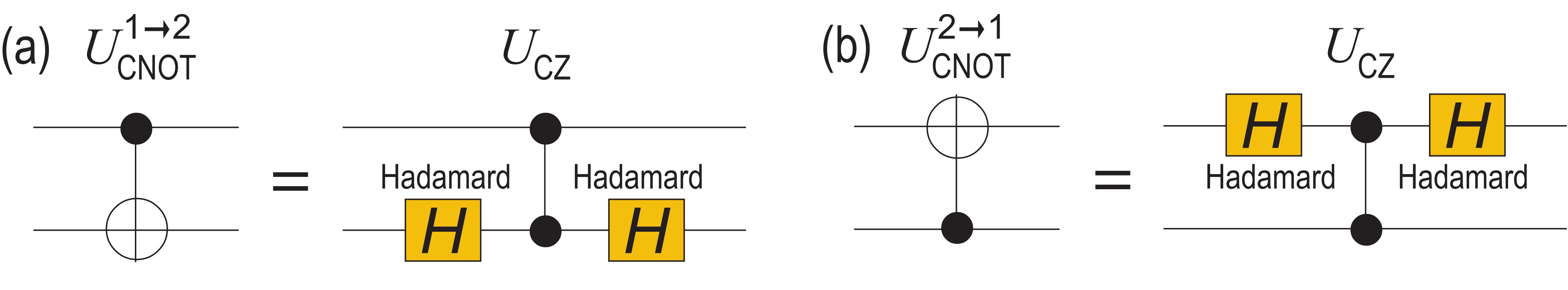
The CNOT gate $U_{\text{CNOT}}^{m\rightarrow m+1}$ is constructed by the sequential applications of the CZ gate and the Hadamard gate as SM

$$U_{\text{CNOT}}^{m\rightarrow m+1}=U_{\text{H}}^{\left(m+1\right)}U_{\text{CZ}}U_{\text{H}}^{\left(m+1\right)},$$

(22)

where the control qubit is the skyrmion in the $m$-layer and and target qubit is the skyrmion in the ($m$+$1$)-layer.

We have so far constructed two-qubit operations between two adjacent qubits. However, it is necessary to construct two-qubit operations between any two qubits. For this it is enough to define the SWAP gate swapping two ajacent qubits such as $U_{\text{SWAP}}^{m\Leftrightarrow m+1}\left|s_{m}s_{m+1}\right\rangle=\left|s_{m+1}s_{m}\right\rangle$. It is decomposed into the sequential application of the CNOT gates SM ,

$$U_{\text{SWAP}}^{m\Leftrightarrow m+1}=U_{\text{CNOT}}^{m\rightarrow m+1}U_{\text{CNOT}}^{m+1\rightarrow m}U_{\text{CNOT}}^{m\rightarrow m+1}.$$

(23)

Then, any two qubits are swapped by an appropriate sequence of these SWAP gates.

Initialization. In order to execute quantum computations, we need to prepare an initial state $\left|00\cdots 0\right\rangle$. We apply an electric field $E_{z}$ to all skyrmions, which resolves the degeneracy between two Bloch-type skyrmions in each layer so that the state $\left|0\right\rangle$ has the lower energy. By cooling down the sample, each qubit falls into the ground state $\left|0\right\rangle$. Hence, after switching off the electric field, the system is initialized as $\left|00\cdots 0\right\rangle$.

Read out process. The read out process of the qubit information could be realized by observing the skyrmion helicity in each layer. By observing the helicity, it is fixed either at $\eta=0$ or $\pi$ because they are two-fold degenerate ground states. The result is $\left|s_{1}s_{2}\cdots s_{N}\right\rangle$. This is a standard representation of the read out process of quantum computations.

Pixelated skyrmion. In the present proposal, it is necessary to control precisely the position of the skyrmion in the execution of the Ising coupling gate. A recent theoretical report has suggested that the position of a nanoscale skyrmion could be digitalized by introducing a square-grid pinning pattern in a thin-film sample hosting a skyrmion Xichao_ComPhys . To be specific, one can fabricate a sample where the easy-axis magnetic anisotropy is modulated with a grid-pattern landscape. The skyrmion is trapped to this grid and thus the center of skyrmion is digitalized. Although this architecture was made for nanoscale skyrmions in ferromagnets with Dzyaloshinskii-Moriya interaction Xichao_ComPhys , it would be also possible to apply it to the system of nanoscale skyrmions in frustrated magnets. Then, the center of the skyrmion is digitalized, which could improve the accuracy of the gate operation.

Discussion and Conclusion. We have proposed a method to materialize the universal quantum gate sets based on the helicity of skyrmions in frustrated magnets. Quantum computations can be performed by temporally controlling the electric field, the spin current, and the skyrmion position.

We estimate the parameters for actual systems. The frustrated skyrmion size is in the range of $3$ nm - $10$ nm. The dipole energy $V$ in Eq.(3) is the order Xichao_NCOMMS2017 of $10^{-21}$J, which is estimated numerically. It corresponds to the order of $100$ K, which is reasonably high temperature. The interlayer exchange interaction $J_{\text{int}}$ is the order of $1$ meV. The required electric field Psa $E_{z}$ is the order of $100$ nV/nm. The required spin current Xichao_NCOMMS2017 $J_{\text{current}}$ is the order of $1$ $\mu$A/nm². The operating time of the quantum gate is governed by the flipping time of the helicity or the dynamics of the center Xichao_NCOMMS2017 , which is the order of $100$ ps.

Although the present work was motivated by a recent theoretical report Psa , the mechanism of the helicity control is quite different. The magnetic DDI plays an essential role in the present work but not in the previous report Psa . We have used the fact that the DDI term favors Bloch-type skyrmions in frustrated magnets. There are two different configurations of Bloch-type skyrmions, which we have used as a qubit. Furthermore, we have proposed the use of electric fields and spin currents in controlling qubits. On the other hand, external magnetic fields are used for the control in the previous proposal. The merit of our method is that electric fields and spin currents can be controlled locally and relatively easily compared to magnetic fields.

M.E. is very much grateful to N. Nagaosa for helpful discussions on the subject. This work is supported by the Grants-in-Aid for Scientific Research from MEXT KAKENHI (Grants No. JP18H03676). This work is also supported by CREST, JST (Grants No. JPMJCR20T2). J.X. was an International Research Fellow of the Japan Society for the Promotion of Science (JSPS). X.Z. was a JSPS International Research Fellow. X.Z. was supported by JSPS KAKENHI (Grant No. JP20F20363). X.L. acknowledges support by the Grants-in-Aid for Scientific Research from JSPS KAKENHI (Grant Nos. JP20F20363, JP21H01364, and JP21K18872). Y.Z. acknowledges support by Guangdong Basic and Applied Basic Research Foundation (2021B1515120047), Guangdong Special Support Project (Grant No. 2019BT02X030), Shenzhen Fundamental Research Fund (Grant No. JCYJ20210324120213037), Shenzhen Peacock Group Plan (Grant No. KQTD20180413181702403), Pearl River Recruitment Program of Talents (Grant No. 2017GC010293), and National Natural Science Foundation of China (Grant Nos. 11974298, 12004320, and 61961136006).

In this Supplemental Material, we summarize matrix representations of quantum gates in the main text.

$\pi/4$ phase-shift gate: The $\pi/4$ phase-shift gate is defined by

$$U_{T}\equiv\left(\begin{array}[]{cc}1&0\\ 0&e^{i\pi/4}\end{array}\right).$$

(S1)

Hadamard gate: The Hadamard gate is defined by

$$U_{\text{H}}\equiv\frac{1}{\sqrt{2}}\left(\begin{array}[]{cc}1&1\\ 1&-1\end{array}\right).$$

(S2)

CZ gate: The CZ gate is defined by

$$U_{\text{CZ}}\equiv\left(\begin{array}[]{cccc}1&0&0&0\\ 0&1&0&0\\ 0&0&1&0\\ 0&0&0&-1\end{array}\right).$$

(S3)

We note that the action is the same whether we choose the control and target qubits as the first or second qubit. Thus, we use a symmetric notation between the first and second qubits as shown in Fig.S1. We construct it based on the Ising interaction. It is given by

$$U_{\text{CZ}}=e^{i\pi/4}U_{Z}^{\left(1\right)}\left(\frac{\pi}{2}\right)U_{Z}^{\left(2\right)}\left(\frac{\pi}{2}\right)U_{\text{ZZ}}\left(-\frac{\pi}{2}\right),$$

(S4)

where we have defined the Ising coupling gate

$$U_{\text{ZZ}}\left(\theta\right)\equiv\exp\left[-\frac{i\theta}{2}\sigma_{z}^{\left(1\right)}\sigma_{z}^{\left(2\right)}\right],$$

(S5)

and the $z$ rotation gate acting on the first qubit

$$U_{Z}^{\left(1\right)}\left(\frac{\pi}{2}\right)=\text{diag.}\left(e^{-i\pi/4},e^{i\pi/4},e^{-i\pi/4},e^{i\pi/4}\right),$$

(S6)

and the $z$ rotation gate acting on the second qubit

$$U_{Z}^{\left(2\right)}\left(\frac{\pi}{2}\right)=\text{diag.}\left(e^{-i\pi/4},e^{-i\pi/4},e^{i\pi/4},e^{i\pi/4}\right).$$

(S7)

CNOT gate: CNOT gate is constructed by the sequential applications of the CZ gate and the Hadamard gate

$$U_{\text{CNOT}}^{1\rightarrow 2}=U_{\text{H}}^{\left(2\right)}U_{\text{CZ}}U_{\text{H}}^{\left(2\right)},$$

(S8)

where the CNOT gate whose control qubit is the first qubit and target qubit is the second qubit is defined by

$$U_{\text{CNOT}}^{1\rightarrow 2}\equiv\left(\begin{array}[]{cccc}1&0&0&0\\ 0&1&0&0\\ 0&0&0&1\\ 0&0&1&0\end{array}\right),$$

(S9)

and $U_{\text{H}}^{\left(2\right)}$ is the Hadamard gate acting on the second qubit

$$U_{\text{H}}^{\left(2\right)}=I_{2}\otimes U_{\text{H}}=\frac{1}{\sqrt{2}}\left(\begin{array}[]{cccc}1&1&0&0\\ 1&-1&0&0\\ 0&0&1&1\\ 0&0&1&-1\end{array}\right).$$

(S10)

The quantum circuit representation of Eq.(S8) is shown in Fig.S1(a).

On the other hand, the CNOT gate whose control qubit is the second qubit and target qubit is the first qubit is defined by

$$U_{\text{CNOT}}^{2\rightarrow 1}\equiv\left(\begin{array}[]{cccc}1&0&0&0\\ 0&0&0&1\\ 0&0&1&0\\ 0&1&0&0\end{array}\right).$$

(S11)

It is constructed as

$$U_{\text{CNOT}}^{2\rightarrow 1}=U_{\text{H}}^{\left(1\right)}U_{\text{CZ}}U_{\text{H}}^{\left(1\right)},$$

(S12)

where $U_{\text{H}}^{\left(1\right)}$ is the Hadamard gate acting on the first qubit

$$U_{\text{H}}^{\left(1\right)}=U_{\text{H}}\otimes I_{2}=\frac{1}{\sqrt{2}}\left(\begin{array}[]{cccc}1&0&1&0\\ 0&1&0&1\\ 1&0&-1&0\\ 0&1&0&-1\end{array}\right).$$

(S13)

The quantum circuit representation of Eq.(S12) is shown in Fig.S1(b).

SWAP gate: So far, we have constructed two-qubit operations between two adjacent qubits. However, it is necessary to construct two-qubit operations between any two qubits. It is executed by the SWAP gate defined by

$$U_{\text{SWAP}}\equiv\left(\begin{array}[]{cccc}1&0&0&0\\ 0&0&1&0\\ 0&1&0&0\\ 0&0&0&1\end{array}\right),$$

(S14)

whose operation is given by$U_{\text{SWAP}}\left|s_{2}s_{1}\right\rangle=\left|s_{1}s_{2}\right\rangle$. It is decomposed to the sequential application of the CNOT gates,

$$U_{\text{SWAP}}=U_{\text{CNOT}}^{1\rightarrow 2}U_{\text{CNOT}}^{2\rightarrow 1}U_{\text{CNOT}}^{1\rightarrow 2},$$

(S15)

whose quantum circuit representation is shown in Fig.S2.

References

- (1) N. Nagaosa and Y. Tokura, Nat. Nanotech. 8, 899 (2013).
- (2) M.Mochizuki and S. Seki, J. Phys.: Condens. Matter 27, 503001 (2015).
- (3) G. Finocchio, F. Büttner, R. Tomasello, M. Carpentieri, and M. Kläui, J. Phys. D: Appl. Phys. 49, 423001 (2016).
- (4) R. Wiesendanger, Nat. Rev. Mat. 1, 16044 (2016).
- (5) A. Fert, N. Reyren, and V. Cros, Nat. Rev. Mater. 2, 17031 (2017).
- (6) Y. Zhou, Natl. Sci. Rev. 6, 210 (2019).
- (7) X. Zhang, Y. Zhou, K. M. Song, T.-E. Park, J. Xia, M. Ezawa, X. Liu, W. Zhao, G. Zhao, and S. Woo, J. Phys. Condens. Matter 32, 143001 (2020).
- (8) B. Göbel, I. Mertig, and O. A. Tretiakov, Phys. Rep. 895, 1 (2021).
- (9) C. Reichhardt, C. J. O. Reichhardt, and M. V. Milosevic, arXiv:2102.10464 (2021).
- (10) S. Li, W. Kang, X. Zhang, T. Nie, Y. Zhou, K. L. Wang, and W. Zhao, Mater. Horiz. 8, 854, (2021).
- (11) Y. Tokura and N. Kanazawa, Chem. Rev. 121, 2857 (2021).
- (12) X. Yu, J. Magn. Magn. 539, 168332 (2021).
- (13) C. H. Marrows and K. Zeissler, Appl. Phys. Lett. 119, 250502 (2021).
- (14) J. Sampaio, V. Cros, S. Rohart, A. Thiaville, and A. Fert, Nat. Nanotechnol. 8, 839 (2013).
- (15) R. Tomasello, E. Martinez, R. Zivieri, L. Torres, M. Carpentieri, and G. Finocchio, Sci. Rep. 4, 6784 (2014).
- (16) X. Zhang, M. Ezawa, and Y. Zhou, Sci. Rep. 5, 9400 (2015).
- (17) A. O. Leonov and M. Mostovoy, Nat. Commun. 6, 8275 (2015).
- (18) S.-Z. Lin and S. Hayami, Phys. Rev. B 93, 064430 (2016).
- (19) C. D. Batista, S.-Z. Lin, S. Hayami, and Y. Kamiya, Rep. Prog. Phys. 79, 084504 (2016).
- (20) H. T. Diep, Entropy 21, 175 (2019).
- (21) X. Zhang, J. Xia, Y. Zhou, X. Liu, H. Zhang, M. Ezawa, Nat. Com. 8, 1717 (2017).
- (22) T. Kurumaji, T. Nakajima, M. Hirschberger, A. Kikkawa, Y. Yamasaki, H. Sagayama, H. Nakao, Y. Taguchi, T.-H. Arima, and Y. Tokura, Science 365, 914 (2019).
- (23) J. Xia, X. Zhang, M. Ezawa, O. A. Tretiakov, Z. Hou, W. Wang, G. Zhao, X. Liu, H. T. Diep, and Y. Zhou, Appl. Phys. Lett. 117, 012403 (2020)
- (24) V. Lohani, C. Hickey, J. Masell, and A. Rosch, Phys. Rev. X 9, 041063 (2019).
- (25) P. Siegl, E. Y. Vedmedenko, M. Stier, M. Thorwart, and T. Posske, arXiv:2110.00348 (2021).
- (26) A. Haller, S. Groenendijk, A. Habibi, A. Michels, and T. L. Schmidt, arXiv:2112.12475 (2021).
- (27) K. Mæland and A. Sudbø, arXiv:2204.02999 (2021).
- (28) C. Psaroudaki and C. Panagopoulos, Phys. Rev. Lett. 127, 06720 (2021).
- (29) S. Heinze, K. von Bergmann, M. Menzel, J. Brede, A. Kubetzka, R. Wiesendanger, G. Bihlmayer and S. Blugel, Nature Physics 7, 713 (2011).
- (30) A. Schlenhoff, P. Lindner, J. Friedlein, S. Krause, R. Wiesendanger, M. Weinl, M. Schreck and M. Albrecht, ACS Nano 9, 5908 (2015).
- (31) A. Roldan-Molina, A. S. Nunez and J. Fernandez-Rossie, New J. Phys. 18, 045015(2016).
- (32) J. Grenz, A. Kohler, A. Schwarz and R. Wiesendanger, Phys. Rev. Lett. 119, 047205 (2017).
- (33) N. Swain, M. Shahzad and P. Sengupta, arXiv:2203.03359.
- (34) R. Bruning, A. Kubetzka, K. von Bergmann, E. Y. Vedmedenko, R. Wiesendanger, arXiv:2201.10702.
- (35) R. Feynman, Int. J. Theor. Phys. 21, 467 (1982).
- (36) D. P. DiVincenzo, Science 270, 255 (1995).
- (37) M. Nielsen and I. Chuang, "Quantum Computation and Quantum Information", Cambridge University Press, (2016); ISBN 978-1-107-00217-3.
- (38) Y. Nakamura; Yu. A. Pashkin; J. S. Tsai, Nature 398, 786 (1999).
- (39) E. Knill, R. Laflamme and G. J. Milburn, Nature, 409, 46 (2001).
- (40) D. Loss and D. P. DiVincenzo, Phys. Rev. A 57, 120 (1998).
- (41) J. I. Cirac and P. Zoller, Phys. Rev. Lett. 74, 4091 (1995).
- (42) L. M.K. Vandersypen, M. Steffen, G. Breyta, C. S. Yannoni, M. H. Sherwood, I. L. Chuang, Nature 414, 883 (2001).
- (43) B. E. Kane, Nature 393, 133 (1998).
- (44) D. Deutsch, Proceedings of the Royal Society A. 400, 97 (1985).
- (45) C. M. Dawson and M. A. Nielsen arXiv:quant-ph/0505030.
- (46) M. Nielsen and I. Chuang, "Quantum Computation and Quantum Information", Cambridge University Press, Cambridge, UK (2010).
- (47) H. Katsura, N. Nagaosa and A. V. Balatsky, Phys. Rev. Lett. 95, 057205 (2005).
- (48) X. Yao, J. Chen and S. Dong, New J. Phys. 22, 083032 (2020).
- (49) See Supplemental Material for explicit matrix representations.
- (50) N. Schuch and J. Seiwert, Phys. Rev. A 67, 032301 (2003).
- (51) Y. Makhlin, Quant. Info. Proc. 1, 243 (2002).
- (52) X. Zhang, J. Xia, K. Shirai, H. Fujiwara, O. A. Tretiakov, M. Ezawa, Y. Zhou, X. Liu, Com. Phys. 4, 255 (2021).
Supplemental Material