Universal Modem Generation with Inherent Adaptability to Variant Underwater Acoustic Channels: a Data-Driven Perspective

We denote the data vector as $\mathbf{s}\in\mathbb{C}^{N\times 1}$ with zero mean and an autocorrelation matrix $\mathbb{E}[\mathbf{s}\mathbf{s}^{H}]=\sigma_{s}^{2}\mathbf{I}_{N}$, where $N$ is the number of subcarriers. The modulated signal $\mathbf{x}\in\mathbb{C}^{M\times 1}$ can be written as

where $\mathbf{\Phi}\in\mathbb{C}^{M\times N}(N\leq M)$ is the modulation matrix.

We construct the baseband signal $x(t)$, which is band-limited to $-B/2\leq f\leq B/2$, by employing a Nyquist interpolation filter.

where $x(m/F_{s})=x[m]$, assumed that the sampling rate $F_{s}\geq B$, and

In practice, we typically use a waveform with a finite duration $T$, which can only be approximately bandlimited. Define $M=\lfloor F_{s}T\rfloor$ as the number of samples taken from $x(t)$ within the time interval $0\leq t\leq T$. We can reformulate $x(t)$ as follows:

Following [8], we assume that $\varepsilon=\|x(t)-\tilde{x}(t)\|^{2}\rightarrow 0$ and thus approximate $x(t)$ by $\tilde{x}(t)$.

The transmitted passband signal can be given by

Following [6], the impulse response of the UWA channel can be determined by

where $P$ denotes the number of propagation paths, $A_{p}(t)$ is the path amplitude and $\tau_{p}(t)$ is the time-varying path delay. Since the duration of a transmitted signal is less than the channel stationary time, $A_{p}(t)$ can be considered as a constant value $A_{p}$, and $\tau_{p}(t)$ can be approximated by

where $a_{p}$ denotes the path-specific Doppler scaling factor and $\tau_{p}$ denotes the constant path delay. As a result, $c(\tau,t)$ can be derived as

The received passband signal is

where the impact of noise is neglected for simplicity in illustration.

The baseband signal $r(t)$ can then be derived as

with a duration of $0\leq t\leq T+T_{g}$ due to the delay spread in the channel. The guard interval $T_{g}$ is given by $T_{g}=[\tau_{p}/(a_{p}+1)]_{\max}$ to prevent interference among different symbols.

Time domain samples $r[m^{\prime}]$ can then be obtained by sampling $r(t)$ at a rate $F_{s}$, where we have

for $m^{\prime}=0,1,\cdots,M^{\prime}-1$, where $M^{\prime}$ denotes the number of signal samples of $r(t)$, which is set as $\left\lfloor F_{s}T+F_{s}T_{g}\right\rfloor$ to capture all useful signals to maximize information retention.

The received vector $\mathbf{r}\in\mathbb{C}^{M^{\prime}\times 1}$ can be written in the matrix-vector notation as follows, including the additive white Gaussian noise $\mathbf{w}\sim\mathcal{CN}(0,\sigma_{n}^{2}\mathbf{I}_{M^{\prime}})$.

$\mathbf{H}\in\mathbb{C}^{M^{\prime}\times M}$ denotes the channel matrix, whose $(m^{\prime},m)\mathrm{th}$ entry is

To simplify the expression, the channel matrix $\mathbf{H}$ can be expressed in another form as

The complex path gain for the $p\mathrm{th}$ path $\xi_{p}\in\mathbb{C}$ is

$\mathbf{\Lambda}_{p}\in\mathbb{C}^{M^{\prime}\times M^{\prime}}$ is a diagonal matrix with an $(m^{\prime},m^{\prime})\mathrm{th}$ entry as

The matrix $\mathbf{\Gamma}_{p}\in\mathbb{C}^{M^{\prime}\times M}$ has an $(m^{\prime},m)\mathrm{th}$ entry as

Here we adopt the notation as $\gamma_{m^{\prime}}^{(p)}=(a_{p}+1)m^{\prime}/F_{s}-\tau_{p}$, noting that when $\gamma_{m^{\prime}}^{(p)}<0$ or $\gamma_{m^{\prime}}^{(p)}>T$, we have

The signal after demodulation $\mathbf{y}\in\mathbb{C}^{N\times 1}$ at the receiver can be expressed as

where $\mathbf{H}_{e}=\mathbf{\Psi}^{H}\mathbf{H\Phi}$ denotes the equivalent channel and $\mathbf{\Psi}^{H}\in\mathbb{C}^{N\times M^{\prime}}$ represents the demodulation matrix, which converts symbols into original dimensions.

Following [6, 11], in the ZP-OFDM system, due to the presence of null subcarriers, the modulation matrix $\mathbf{\Phi}_{\mathrm{OFDM}}\in\mathbb{C}^{M\times N}$ typically has fewer columns than rows, which can be split into two parts

$\mathbf{F}_{M}$ denotes the discrete Fourier transform (DFT) matrix with the $(i,j)$th entry

$\mathbf{X}\in\mathbb{C}^{M\times N}$ represents the matrix to extract $N$ columns from $\mathbf{F}_{M}^{H}$, ensuring the selected subcarriers are as evenly distributed as possible within the passband.

The demodulation matrix $\mathbf{\Psi}^{H}\in\mathbb{C}^{N\times M^{\prime}}$ can be written as

where $\mathbf{R}\in\mathbb{C}^{M\times M^{\prime}}$ represents the matrix to append the last $L=M^{\prime}-M$ columns of $\mathbf{X}^{H}\mathbf{F}_{M}$ on its front.

We aim to identify the modem structure (i.e. modulation matrix $\mathbf{\Phi}$ and demodulation matrix $\mathbf{\Psi}^{H}$), which will optimize system performance across various channel matrices $\mathbf{H}$. Therefore, we need to establish an appropriate evaluation criterion to model the optimization problem, where the equivalent sub-channel rate proves to be useful, following [9].

The signal after demodulation $\mathbf{y}$ can be segmented into $N$ sub-channels, each subject to interference and noise. The output of the $n\mathrm{th}$ sub-channel, denoted by $\mathbf{y}[n]$, can be expressed as

where the last two terms of the sum represent interference and noise, respectively.

Since we find the worst sub-channel has a more significant impact on the transmission, the criterion function is defined as

where $K\geq 1$ denotes the amplification factor of the worst sub-channel rate.

where $r_{n}$ denotes the $n$th equivalent sub-channel rate, which is related to the signal-to-noise ratio (SNR) $\sigma_{s}^{2}/\sigma_{n}^{2}$. Hence, the modulation design can be formulated as an optimization problem

Where $\mathbb{E}_{\mathbf{H}}[\cdot]$ represents the expectation conditioned on the distribution of $\mathbf{H}$, we introduce deep learning-based methods to approximate the quasi-optimal solution.

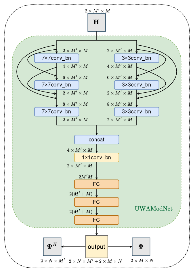
As demonstrated in Fig. 1, we propose a multi-resolution network since the energy distribution of $\mathbf{H}$ exhibits significant localization characteristics. In regions where the energy distribution is more concentrated, smaller convolutional kernels are better able to extract finer features, while in regions where the energy distribution is not concentrated, larger convolutional kernels are adequate. The UWA channel matrix $\mathbf{H}$ is processed as an input image with dimensions $2\times M^{\prime}\times M$. This image comprises two channels, representing the real and imaginary parts of $\mathbf{H}$. The input image is then processed through two parallel pathways. The first pathway consists of three sequential $7\times 7$ convolutional layers that generate a high-resolution view. In contrast, the second pathway includes three consecutive $3\times 3$ convolutional layers, resulting in a lower resolution. Each convolution is followed by a batch normalization, and a dense connection is employed among the convolution layers, alleviating the over-fitting problem. The outputs from both pathways are then concatenated and integrated using a $1\times 1$ convolutional layer. Subsequently, three fully connected (FC) layers are incorporated to adjust the output size, which is finally divided into $\mathbf{\Phi}$ and $\mathbf{\Psi}^{H}$. The energies of $\mathbf{\Phi}$ and $\mathbf{\Psi}^{H}$ are normalized to $N$ and $NM^{\prime}/M$, respectively, aligning with the ZP-OFDM standards.

It is worth noting that each layer, except for the final fully connected (FC) layer, is followed by a leaky ReLU activation layer to introduce non-linearity. Leaky ReLU is defined as

where the negative slope, denoted as $\beta$, is set to a default value of 0.3.

Within the specified range of channel parameters, our goal is to obtain definite modulation matrix $\mathbf{\Phi}$ and demodulation matrix $\mathbf{\Psi}^{H}$. However, when we simultaneously aim to optimize system performance and ensure the convergence of system outputs, the training outcomes are not entirely satisfactory. Thus, we have revised our training strategy: In Stage I, we focus on enhancing system performance, and in Stage II, we address both system performance and the convergence of system outputs, as is developed in Algorithm 1 where $E_{1}$ and $E_{2}$ denote the training epochs of Stage I and Stage II respectively.

In this section, we describe the UWA channel parameters employed to create the training and validation datasets, some of which are displayed in Table I, partially following [8].

Based on the parameters in Table I, we deduce that $M=\left\lfloor F_{s}T\right\rfloor=128$, $M^{\prime}=\left\lfloor F_{s}T+F_{s}T_{g}\right\rfloor=228$, and thus the number of null subcarriers $M-N=58$. In addition, following [8], the path amplitude $A_{p}$ is distributed as $A_{p}\stackrel{{\scriptstyle i.i.d}}{{\sim}}\mathcal{CN}(0,1)$, the path delay $\tau_{p}$ follows a uniform distribution $\tau_{p}\stackrel{{\scriptstyle i.i.d}}{{\sim}}\mathcal{U}(0,\tau_{\max})$, and the path Doppler scaling factor $a_{p}$ conforms to a uniform distribution $a_{p}\stackrel{{\scriptstyle i.i.d}}{{\sim}}\mathcal{U}(1/(1+a_{\max})-1,a_{\max})$ for $p=1,2,\cdots,P$.

The training dataset consists of 15,000 UWA channel matrices $\mathbf{H}$ and their corresponding equivalent channel matrices for the ZP-OFDM system $\mathbf{H}_{e,\mathrm{OFDM}}$. The validation dataset contains 5,000 pairs of $\{\mathbf{H},\mathbf{H}_{e,\mathrm{OFDM}}\}$. The training set is used to adjust UWAModNet weights, while the validation set helps to evaluate the performance during training and finalize the learned modem. Additionally, a testing dataset with 10,000 pairs of $\{\mathbf{H},\mathbf{H}_{e,\mathrm{OFDM}}\}$ is used to generate equivalent sub-channel rate curves and bit error rate curves for system performance evaluation. The process of generating a pair of $\{\mathbf{H},\mathbf{H}_{e,\mathrm{OFDM}}\}$ is shown in Algorithm 2.

For other parameters, the amplification factor $K$ in equation (25) is set to 10 by default. The Adam optimizer, configured with $\beta_{1}=0.9,\beta_{2}=0.999$, learning rate $lr=1\times 10^{-3}$, and $\epsilon=1\times 10^{-8}$, is used to train UWAModNet. Furthermore, both Stage I and Stage II of our training are configured with 400 epochs and a batch size of 100, with our UWAModNet operating at a signal-to-noise ratio (SNR) of 20 dB.

In this section, two figures are presented to demonstrate the performance of the learned modem, one showing the equivalent sub-channel rate and the other depicting the bit error rate.

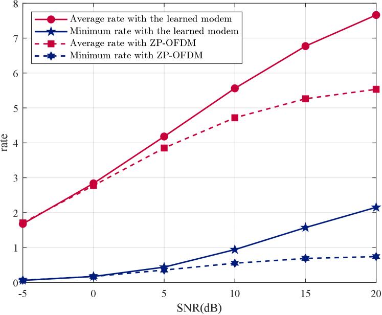
Fig. 2 shows how average and minimum equivalent sub-channel rates vary with SNR ranging from -5 to 20 dB with $a_{\max}=0.001$. At an SNR of 20 dB, the learned modem enhances the average equivalent sub-channel rate by 38.5% and boosts the minimum equivalent sub-channel rate by 190.8% compared to ZP-OFDM. The figure demonstrates that the learned modem achieves a higher average and minimum rate, indicating significant improvements in overall and worst performance.

As for the bit error rate, at the transmitter, the bit sequence $\mathbf{b}$ is translated to the symbol sequence $\mathbf{s}$ using QPSK constellation mapping with Gray coding. At the receiver, we perform linear zero-forcing (LZF) equalization on the demodulated signal $\mathbf{y}$ as follows.

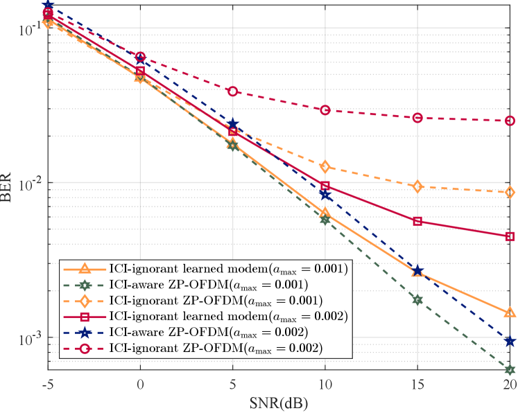
where $\mathbf{z}$ denotes the output of the equalizer. We show the performance of both ICI-aware LZF equalization ($\hat{\mathbf{H}}=\mathbf{H_{e}}$) and ICI-ignorant one-tap LZF equalization ($\hat{\mathbf{H}}=\mathrm{diag}(\mathbf{H_{e}})$) under constraints $a_{\max}=0.001$ and $a_{\max}=0.002$.

In Fig. 3, the learned modem achieves comparable BER performance to ICI-aware ZP-OFDM but at a lower computational cost, and it significantly outperforms ICI-ignorant ZP-OFDM. At an SNR of 20 dB, with $a_{\max}=0.001$, the learned modem declines BER by 84% compared to ICI-ignorant ZP-OFDM.

Under poorer channel conditions, with $a_{\max}=0.002$, the learned modem, originally trained at $a_{\max}=0.001$, suffers some performance loss but still outperforms ICI-ignorant ZP-OFDM, demonstrating good robustness.

References

- [1] J. Xu, M. A. Kishk, and M.-S. Alouini, “Coverage enhancement of underwater internet of things using multilevel acoustic communication networks,” IEEE Internet of Things Journal, vol. 9, no. 24, pp. 25 373–25 385, 2022.
- [2] X. Wang, X. Shi, J. Wang, and Z. Sun, “Iterative lmmse-sic detector for dse-aware underwater acoustic otfs systems,” IEEE Transactions on Vehicular Technology, vol. 73, no. 7, pp. 9895–9910, 2024.
- [3] C. Zhang, Y. Xie, D. Mishra, T. Pacino, J. Shao, B. Li, J. Yuan, P. Chen, and Y. Rong, “A low complexity channel emulator for underwater acoustic communications,” in OCEANS 2023 - MTS/IEEE U.S. Gulf Coast, 2023, pp. 1–8.
- [4] H. L. Nguyen Thi, Q. Khuong Nguyen, and V. D. Nguyen, “A combination of time and frequency synchronization with doppler compensation for coded ofdm-based uwa systems,” in 2023 Asia Pacific Signal and Information Processing Association Annual Summit and Conference (APSIPA ASC), 2023, pp. 1304–1309.
- [5] M. Wen, X. Cheng, L. Yang, Y. Li, X. Cheng, and F. Ji, “Index modulated ofdm for underwater acoustic communications,” IEEE Communications Magazine, vol. 54, no. 5, pp. 132–137, 2016.
- [6] B. Li, S. Zhou, M. Stojanovic, L. Freitag, and P. Willett, “Multicarrier communication over underwater acoustic channels with nonuniform doppler shifts,” IEEE Journal of Oceanic Engineering, vol. 33, no. 2, pp. 198–209, 2008.
- [7] X. Wang and J. Wang, “Pilot allocation for mimo-zp-ofdm systems in underwater acoustic channel based on structured compressive sensing,” in 2016 IEEE/OES China Ocean Acoustics (COA), 2016, pp. 1–5.
- [8] A. K. P., C. R. Murthy, and P. Muralikrishna, “Variable bandwidth multicarrier communications: A new waveform for the delay-scale channel,” in 2022 IEEE 23rd International Workshop on Signal Processing Advances in Wireless Communication (SPAWC), 2022, pp. 1–5.
- [9] H. Zhang, X. Wang, J. Tan, and J. Wang, “Modem optimization of high-mobility scenarios: A deep-learning-inspired approach,” in 2024 IEEE International Conference on Communications Workshops (ICC Workshops), 2024, pp. 1–6.
- [10] Z. Lu, J. Wang, and J. Song, “Multi-resolution csi feedback with deep learning in massive mimo system,” in ICC 2020 - 2020 IEEE International Conference on Communications (ICC), 2020, pp. 1–6.
- [11] C. R. Berger, S. Zhou, J. C. Preisig, and P. Willett, “Sparse channel estimation for multicarrier underwater acoustic communication: From subspace methods to compressed sensing,” IEEE Transactions on Signal Processing, vol. 58, no. 3, pp. 1708–1721, 2010.