Unity is Power: Semi-Asynchronous Collaborative Training of Large-Scale Models with Structured Pruning in Resource-Limited Clients
Abstract
In this work, we study to release the potential of massive heterogeneous weak computing power to collaboratively train large-scale models on dispersed datasets. In order to improve both efficiency and accuracy in resource-adaptive collaborative learning, we take the first step to consider the unstructured pruning, varying submodel architectures, knowledge loss, and straggler challenges simultaneously. We propose a novel semi-asynchronous collaborative training framework, namely , with data distribution-aware structured pruning and cross-block knowledge transfer mechanism to address the above concerns. Furthermore, we provide theoretical proof that can achieve asymptotic optimal convergence rate of . Finally, we conduct extensive experiments on a real-world hardware testbed, in which 16 heterogeneous Jetson devices can be united to train large-scale models with parameters up to 0.11 billion. The experimental results demonstrate that improves accuracy by up to 8.8% and resource utilization by up to 1.2 compared to state-of-the-art methods, while reducing memory consumption by approximately 22% and training time by about 24% on all resource-limited devices.
1 Introduction
The pretrained foundation models (PFMs) with a huge amount of parameters, such as ChatGPT, GPT-4, have witnessed great success in various fields [16, 42, 23], which demonstrates superior performance on kinds of downstream tasks, such as CV [32], NLP [3], robotics [8], etc. However, training the large-scale pretrained models is becoming increasingly more expensive, usually requiring scaling to thousands of high-performance GPUs.
In real-world scenarios, heterogeneous weak computing power are commonly everywhere, such as mobile devices, equipped with limited computational and memory resources. Hence, it would be difficult and unaffordable for resource-constrained clients to train the full large-scale models. In addition, the resource-limited devices can produce heterogeneous data and bring "data silos" due to the promulgation of rigorous data regulations such as GDPR [30]. Therefore, a practical problem arises: How to release the potential of massive resource-limited devices to train large-scale models uniting the weak computing power and heterogeneous dispersed datasets collaboratively?
Traditionally, fruitful works have explored the lightweight collaborative training methods, such as quantization [25, 20, 40], compression [10, 15], distillation [26, 6], and pruning strategies [37]. In addition, adaptively splitting the globally large models into submodels can facilitate the collaboration process in resource-limited federated learning (FL), such as RAM-Fed [31], PruneFL [14], OAP [43], pFedGate [5]. However, when deploying the mentioned methods to prune the large-scale models

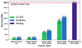
in real-world resource-limited hardware, both efficiency and accuracy should be carefully considered, arising some tricky challenges. (1) Unstructured pruning. The existing adaptive splitting methods adopt unstructured pruning [12, 13], which only zeros out unimportant parameters without reducing the original parameter size. As shown in Fig.1, unstructured pruning fails to train the splitted submodels due to memory constraints in real-world hardware. (2) Varying submodel architectures. The randomized or weight-based submodels might not fit the heterogeneous data distributions in each client, which limits the learning potential of the generated submodels. (3) Knowledge loss. The shallow submodels fail to learn high-level and complex knowledge due to the sparsity of the submodel architectures, causing knowledge loss in the resourced-limited clients. (4) Straggler. The limited computation abilities of clients can cause enormous disparities in submodels training time, slowing down the large model’s convergence and lowering down the utilization of dispersed computing power.
Along this line, in this work, we propose a novel Semi-asynchronous Collaborative training framework with Structured Pruning, named , which can release the potential of massive heterogeneous resource-limited computing power to train a globally large model. In detail, designs a data distribution-aware structured pruning algorithm to ensure a balanced learning capability of submodels at both depth and width dimensions and accelerate the training process. The server first prunes the blocks of the large models in a rolling fashion according to the available resources of clients. Then, the clients train the structured width-based segment-wise masks based on dispersed datasets to make the submodels fit the heterogeneous data distributions. Considering the knowledge loss of the pruned submodels in the resource-limited clients, we adopt self-distillation to implement cross-block knowledge transfer. To facilitate resource utilization and mitigate the straggler challenge, we design a semi-asynchronous aggregation strategy to further accelerate the large model convergence. Furthermore, we give a detailed convergence analysis of , which can achieve an asymptotically optimal rate . Finally, we deploy on a real-world hardware testbed, in which 16 heterogeneous Jetson devices can be united to train a large-scale model with parameters up to 0.11 billion (B), demonstrating its superiority compared with the state-of-the-arts, while effectively reducing memory usage and training time. The main contributions are summarized as follows:
-
•
To release the potential of massive heterogeneous weak computing power to train large-scale models on dispersed datasets, we take the first step to improve both the efficiency and accuracy of the collaborative training by considering the unstructured pruning, varying submodel architectures, knowledge loss, and straggler challenges into a united framework.
-
•
We propose a semi-asynchronous collaborative training framework , in which the data distribution-aware structured pruning is designed at both depth and width dimensions while accelerating training. In addition, the structured pruned submodels are trained with self-distillation to implement cross-block knowledge transfer.
-
•
We theoretically prove the strategy can converge with , which shows that our semi-asynchronous aggregation strategy mitigates the straggler problem while balancing the convergence rate.
-
•
We conduct extensive experiments on a real-world hardware testbed, in which 16 Jetson devices can be united to train large-scale models with parameters up to 0.11B. improves accuracy up to 8.8% and resource utilization up to 1.2 compared with the state-of-the-art methods while reducing memory consumption and training time significantly.

2 Related Work
Lightweight Collaborative Training. With the popularity of PFMs, it would be unaffordable for resource-limited devices to train the full model under classic collaborative learning. In recent years, fruitful works have been proposed for lightweight collaborative training such as quantization [25, 40, 20], compression [19, 10, 15] and distillation [26, 6]. Moreover, some works design pruning strategies [12, 14, 37] and mask strategies [17, 13, 5] to adapt to the limited resources, but fail to accelerate the training process due to the unstructured pruning. To ensure both efficiency and accuracy, we introduce personalized trainable structured masks based on local data distribution, so as to better adapt to local limited resources and accelerate the model training process.
Asynchronous Collaborative Training. In the collaborative training scenario, each client usually has heterogeneous resources such as dispersed data or computational power. Therefore, the stragglers can slow down the whole training process, causing the server to wait for updates from all the clients. Therefore, some fully asynchronous methods [33, 45] and semi-asynchronous collaborative training works such as [35, 4, 24, 41, 29] have been proposed to solve the straggler problem. In our work, we design a novel semi-asynchronous aggregation strategy to accelerate collaborative training and mitigate the impact of stale clients simultaneously.
3 Problem Formulation
In this paper, we aim to train globally large models collaboratively while optimizing the utilization of diverse discrete resource-limited computing power. Specifically, we assume there exist clients with different resources and locally heterogeneous datasets , where denotes the -th training data sample and its ground truth label, and . In the resource-limited collaborative learning scenario, we aim to solve the following optimization problem:
| (1) |
where and are the parameters of global model and pruned submodels respectively. , where is the loss function.
4 Framework Design
We propose a semi-asynchronous collaborative training framework , as shown in Fig.2. In , we design a data distribution-aware structured pruning algorithm to ensure a balanced learning capability of submodel at both the depth and width dimensions while accelerating training (Sec.4.1). The server first prunes blocks in a rolling fashion according to the available resources of clients. Then, in order to make submodels fit the heterogeneous data distributions, the clients train structured width-based segment-wise masks based on local datasets. Considering the knowledge loss in resource-limited clients, we train submodels with self-distillation to implement cross-block knowledge transfer (Sec.4.2). Finally, to mitigate the problem of straggler, we design a semi-asynchronous aggregation strategy (Sec.4.3).
4.1 Data Distribution-Aware Structured Pruning

In this section, we focus on the balanced structured pruning of the globally large models at both depth and width dimensions, as shown in Fig.3. For the heterogeneous clients with weak computing power, we obtain the overall pruned rate according to the available resources, which consists of the width pruned rate and the depth pruned rate . The pruned rate is defined as the ratio of the structured-pruned model size of the full model size. For client , the server first generates the depth-pruned submodel with consecutive trainable blocks by freezing the shallow blocks bottom-to-top and pruning the deep blocks top-to-bottom in a rolling fashion.
Then in order to make the submodels fit the heterogeneous data distributions, the clients train the width-based structured masks based on the local data distributions. A Transformer-like model mainly consists of linear layers and Multi-head Self-Attention(MSA) layers. Consequently, we design trainable segment-wise masks for two types of layers, where the segment represents part parameters of linear layer or head in MSA layer. We denote the weight matrix and its binary mask by and respectively, where represents the -th layer. For the linear layer, each value of indicates whether the part of the layer is pruned or not. For the MSA layer, each value of indicates whether the head is pruned or not and represents the number of heads.
However, considering that the segment-wise mask is a binary tensor, directly applying the existing back-propagation methods to model training would lead to gradients backward errors. Inspired by [44, 13], we introduce the corresponding segment-wise importance mask and segment-wise probability mask . To enable back-propagation, we apply the sigmoid function scaling to the importance mask, and further use the Bernoulli distribution [7] to generate the binary mask . Then we use the inverse of the sigmoid function and record with the straight-through estimator [2] for back-propagation.
Furthermore, the binary matrix mask is introduced as an extension of to produce Hadamard product with the weight matrix of the model. For training the personalized mask efficiently, we freeze the corresponding weights of the depth-pruned submodels. Considering the resource-limited problem, we use the submodel size to reflect computation and communication costs. The loss function is as follows:
| (2) |
where represents the cross entropy loss for target class , represents the set of the linear layers and the MSA layers. is the hyperparameter that indicates the extent to which the submodel adapts to the limited resource. For each client, stays as close as possible to to ensure a balanced learning capability of submodel.
Finally, we perform Hadamard product for the depth-pruned submodel and binary matrix to obtain the structured-pruned submodel. The structured pruning strategy significantly reduces the capacity of model, saves storage and computation resources, and accelerates directly on resource-limited clients.
4.2 Self-Distillation based Knowledge Transfer
To mitigate the knowledge loss problem in resource-limited clients, introduces lightweight self-distillation mechanism [38] to implement cross-block knowledge transfer. For the structured-pruned submodel, we place multiple classifiers at specific depths , where , and is the number of the frozen blocks and is the number of blocks in the global model. We use self-distillation by treating the deepest classifier as the teacher and other classifiers as the students. The loss function for the width pruning is as follows:
| (3) |
where is the number of classifiers in client , represents the cross entropy loss of the -th classifier for target class . , temperature t is a hyperparameter that controls the information capacity of data distributions provided by the teacher, indicates the balance the cross entropy loss and self-distillation. The self-distillation mechanism enables the shallow blocks to be equipped with high-level knowledge without extra forward overhead, because the blocks share feature maps.
4.3 Semi-Asynchronous Aggregation Strategy
Due to the stragglers, we design a semi-asynchronous aggregation strategy with minimum ratio of received clients and waiting interval to balance the performance of the collaborative training and the resource utilization of all clients, which is shown in Algorithm 1. After the server receives client updates, it turns on the clock timing and waits for seconds before aggregation.
Considering that the updates may be too stale and deviate significantly from the latest global model, for received gradients, we compute a segment importance score on each trained segment as follows:
| (4) |
where is the gradients of the client on segment in -th round that indicates the extent of updating, represents the weights of the global model on segment in -th round. represents the weights of the global model on segment in the -th round, is the delay round that the client has not taken part in global aggregation. indicates the difference of the received model by the client and the latest model.
Finally, the server aggregates the gradients and updates segment by normalizing the segment important scores on segment as follows:
| (5) |
where represents the set of clients training segment in the -th round, is the learning rate for training the masked submodel. It is worth noting that the aggregation strategy also transfers the high-order knowledge from the deep blocks to shallow blocks in all clients.
5 Convergence Analysis
In this section, we show the convergence rate of our proposed semi-asynchronous collaborative learning framework . The detailed proof is in Appendix C. Firstly, we give a crucial definition for theoretical analysis:
Definition 1.
(Maximum delay). We define the delay as the client has not taken part in the global aggregation for rounds, so we can get:
| (6) |
Then, we give assumptions for ease of convergence analysis:
Assumption 1.
(-smooth). Every function is -smooth for all
| (7) |
Assumption 2.
(Bounded variance). There exists :
| (8) |
bounds the variance of stochastic gradient.
Assumption 3.
(Bounded data heterogeneity level). There exists :
| (9) |
bounds the effect of heterogeneous data.
Assumption 4.
(Bounded gradient). In algorithm 2, the expected squared norm of stochastic gradients is bounded uniformly, for constant and :
| (10) |
With these definitions and assumptions, we can bound the deviation of the average squared gradient norm for the convergence analysis of .
Theorem 1.
Let all assumptions hold. Suppose that the step size satisfies the following relationships:
Therefore, the step size is defined as:
Then, for all , we have :
where , is the number of segment, , means the minimum number of submodels training the corresponding segment in all rounds.
Theorem 1 shows the convergence of the semi-asynchronous aggregation mechanism in with the upper bound on the average gradient of all segments.
Remark 1.
Impact of the maximum delay . As we defined, is the maximum delay between all clients until round . The result indicates that the larger is, the worse the convergence rate is. Taking into account the local training of the submodel, the larger means that the initial local submodels are more biased towards the latest global model. And a smaller is beneficial to the convergence but disturbed by stragglers. Therefore, our semi-asynchronous aggregation balances the convergence rate and the resource utilization.
| Methods | (ViT-Tiny/16)-ImageNet200 | (ViT-Base/16)-ImageNet300 | ||||||||||||
| Server(%) | Client(Avg.)(%) | Server(%) | Client(Avg.)(%) | |||||||||||
| FA(Full) | 38.7 | 63.6 | 37.3 | 39.2 | 64.1 | 37.1 | 63.5 | 68.6 | 87.2 | 68.1 | 64.4 | 83.2 | 62.8 | 60.0 |
| FA+PLATON | 19.3 | 42.7 | 19.1 | 16.5 | 37.5 | 17.4 | 70.4 | 37.6 | 58.2 | 35.5 | 34.5 | 54.2 | 30.1 | 74.3 |
| FA+AdaViT | 17.9 | 36.1 | 16.2 | 14.3 | 34.5 | 14.0 | 67.3 | 31.9 | 54.9 | 32.1 | 28.6 | 51.7 | 29.1 | 72.7 |
| FA+Q-ViT | 17.6 | 40.1 | 15.8 | 14.9 | 34.8 | 13.6 | 70.7 | 29.7 | 52.6 | 29.8 | 25.6 | 49.1 | 26.3 | 74.5 |
| FedPM | 16.2 | 38.7 | 15.5 | 14.2 | 34.0 | 12.9 | 71.8 | 26.4 | 49.3 | 27.2 | 23.7 | 44.8 | 24.6 | 76.2 |
| PruneFL | 21.8 | 42.2 | 19.1 | 20.2 | 39.1 | 17.1 | 69.2 | 42.1 | 65.8 | 41.3 | 37.1 | 61.6 | 36.2 | 79.6 |
| RAM-Fed | 23.6 | 46.0 | 21.5 | 19.4 | 41.2 | 19.3 | 69.9 | 43.4 | 66.7 | 42.0 | 36.8 | 59.6 | 35.3 | 80.5 |
| FedRolex | 24.3 | 48.0 | 23.1 | 20.7 | 45.8 | 20.5 | 72.5 | 44.2 | 67.5 | 43.4 | 38.4 | 62.1 | 38.6 | 82.4 |
| 33.1 | 59.2 | 31.9 | 31.8 | 56.6 | 30.5 | 87.9 | 50.6 | 76.4 | 48.9 | 47.2 | 72.5 | 45.5 | 92.4 | |
| (Async.) | 27.7 | 53.2 | 27.3 | 26.7 | 49.8 | 26.7 | 100.0 | 47.6 | 71.9 | 46.3 | 44.1 | 68.4 | 42.6 | 100.0 |
Next, by choosing the appropriate convergence rate , we can obtain the following corollary.
Corollary 1.
Let all assumptions hold. Supposing that the step size and is sufficiently small, when the constant exists, the convergence rate can be expressed as follows:
Remark 2.
Impact of the minimum participation rate . The Corollary 1 shows that the semi-asynchronous aggregation mechanism in can converge to , while we use the semi-asynchronous aggregate mechanism with the personalized mask trained on local data. The result shows that the larger is, the faster the convergence rate is. Otherwise, it’s obvious that . When , all clients take part in all the communication rounds, which achieves the same convergence rate as asynchronous full client participation FedAvg.
6 Experiments
6.1 Experimental Settings

Testbed Implementation. To effectively demonstrate the real-world applicability of the proposed collaborative training framework, we utilize a GeForce RTX 3090 GPU as the server for aggregation and 4 types of 16 Jetson developer kits as the resource-limited clients to build a real-world testbed, as shown in Fig.4. The details are shown in Tab.5 of Appendix.D.
Baselines. To fully evaluate the performance and efficiency of the proposed framework , we choose the classical FL algorithm FedAvg [21]. Additionally, we combine FedAvg with existing standalone training for sparsifying transformer-like models: PLATON [39], AdaViT [22] and Q-ViT [18], named . Moreover, we evaluate against several FL algorithms designed for resource-limited scenarios, including FedPM [13], PruneFL [14], RAM-Fed [31] and FedRolex [1].
Backbones and datasets. We use three ViT [9] variants with different capabilities, as shown in Tab.4. We conduct experiments based on ImageNet200 and ImageNet300 sampled from ImageNet1K [27] and design a evaluation metric for the real-world testbed, namely Resource Utilization Rate (RU).
We deploy and all baselines on the testbed based on the general FL framework NVFlare [28]. Considering that the unstructured baselines fail to work in the resource-limited clients, we replace the unstructured pruning in the baselines with the structured pruning. We conduct three groups of real-world experiments, and the detailed configurations are shown in Tab.6 and Tab.7. Due to limited space, please refer to Appendix D for additional details of experimental implementation.
| Methods | Server | Client(Avg.) | |||||
| FedAvg(Full) | 56.4 | 78.3 | 55.8 | 50.4 | 73.0 | 49.9 | 61.4 |
| FedAvg+PLATON | 32.3 | 55.3 | 31.6 | 30.7 | 51.8 | 31.6 | 75.1 |
| FedAvg+AdaViT | 31.4 | 54.3 | 31.9 | 30.8 | 51.4 | 29.3 | 74.4 |
| FedAvg+Q-ViT | 30.7 | 53.2 | 30.2 | 28.1 | 52.1 | 27.6 | 74.1 |
| FedPM | 27.3 | 52.2 | 26.3 | 25.4 | 49.1 | 24.1 | 73.6 |
| PruneFL | 34.3 | 58.4 | 32.8 | 31.0 | 54.4 | 30.4 | 76.9 |
| RAM-Fed | 36.4 | 60.8 | 35.5 | 30.4 | 53.1 | 30.1 | 77.5 |
| FedRolex | 38.1 | 63.2 | 37.3 | 35.6 | 58.5 | 34.7 | 78.2 |
| 46.9 | 72.5 | 46.0 | 45.7 | 67.5 | 44.5 | 90.6 | |
| (Async.) | 43.4 | 68.2 | 43.6 | 41.3 | 65.6 | 41.5 | 100.0 |
6.2 Overall Performance
Server’s Performance. As shown in Tab.1 and Tab.2, outperforms all baselines in terms of global performance across three groups of experiments: (1) improves Top1 accuracy of global model by 8.8%/6.4%/8.7% compared to the closest baseline FedRolex in three groups of experiments respectively, demonstrating that our algorithm achieves better generalization in resource-limited scenarios. (2) For Top1 accuracy, the baselines significantly decrease compared to the federated resource-adaptive methods, indicating that the mixed heterogeneity of collaborative training scenarios has severe implications for model training. (3) Considering Top1 accuracy, achieves 5.4%/3.0%/3.5% higher improvement compared to the fully asynchronous algorithm on three groups of experiments respectively. This highlights that effectively balances resource utilization and model performance.
 |
 |
 |
| (a) Convergence Curves | (b) Memory Usage | (c) Training Time |
Clients’ Average Performance. As shown in Tab.1 and Tab.2, outperforms all baselines in terms of weighted average performance of the clients in three groups of experiments: (1) For Top1 accuracy, achieves 11.1%/8.8%/10.1% higher personalized submodel performance compared to the closest baseline FedRolex in three groups of experiments respectively, demonstrating that our framework obtains a better personalized mask for each client in resource-limited scenarios. (2) Comparing the difference between global and local performance, has closer gap than all baselines. This is because the trainable masks better adapt to local data distributions and the depth-pruned submodels in resource-limited clients. (3) Considering Top1 accuracy, achieves 5.1%/3.1%/4.4% higher personalized model performance compared to the designed asynchronous methods on three groups of experiments respectively, which demonstrates that achieves a better balance between resource utilization and personalized submodel performance.
Efficiency Comparison. As shown in Tab.1, Tab.2 and Fig.5, outperforms all baselines in terms of efficiency in three groups of experiments: (1) Compared to FedRolex, reduces memory consumption by about 22% and training time per round by about 24% on all resource-limited devices, demonstrating the superiority of the structured pruning in memory and computation efficiency. (2) For resource utilization rate, achieves 1.4, 1.5, and 1.5 improvements compared to FedAvg and 1.2, 1.1, and 1.2 improvements compared to FedRolex across the three groups of experiments. This demonstrates that the proposed semi-asynchronous aggregation strategy can effectively improve the resource utilization during large-scale model training.
6.3 Ablation Study
| Trainable Mask | Self- dist. | Server(%) | Client(Avg.)(%) | |||||
| Linear | MSA | |||||||
| ✗ | ✗ | ✓ | 22.5 | 45.3 | 21.6 | 18.9 | 40.2 | 18.3 |
| ✗ | ✓ | ✓ | 26.5 | 51.6 | 26.0 | 24.3 | 47.2 | 25.8 |
| ✓ | ✗ | ✓ | 27.8 | 55.4 | 26.8 | 25.3 | 50.9 | 24.9 |
| ✓ | ✓ | ✗ | 28.2 | 56.1 | 26.9 | 22.3 | 47.5 | 21.6 |
| ✓ | ✓ | ✓ | 33.1 | 59.2 | 31.9 | 31.8 | 56.6 | 30.5 |
Effectiveness of trainable mask policies. We validate that the trainable mask strategy is effective in improving global performance and generating personalized masks in resource-limited scenarios. We replace the trainable masking strategies with randomly mask strategies and report the results in Tab.3. We observe that replacing any set of trainable masks with randomized ones leads to a performance decrease. With MSA/Linear/Both Random, improves global model accuracy by 5.3%/6.6%/10.6%, and the average accuracy of submodels on the client by 6.5%/7.5%/12.9% in Top1 accuracy. These confirm the effectiveness of the trainable mask strategy.
Effectiveness of self-distillation mechanism. We validate that the self-distillation mechanism helps shallow submodels on resource-limited clients to learn high-level and complex knowledge. As shown in Tab.3, improves Top1 accuracy by 4.9% for the global performance and by 9.5% for the average performance of submodels. This demonstrates the effectiveness of self-distillation in enabling shallow models on resource-limited clients to obtain more complex and high-level knowledge.
6.4 Hyperparameter Analysis

Impact of minimum received ratio and waiting interval . We study the impact of and on model performance and the resource utilization of the system. As shown in Fig.6, increasing or , improves the performance of both the global model and the submodels, but reduces the resource utilization rate due to requiring a longer wait for the other clients. In addition, we provide more hyperparameter analysis details of weight term of , balance term of and the ratio between of and in Appendix F.2.
7 Conclusion
To release the potential of massive resource-limited nodes, we proposed a novel semi-asynchronous collaborative training framework . We designed a data distribution-aware structured pruning to ensure balanced learning capability and accelerate training. By self-distillation, facilitated shallow blocks obtaining the high-level knowledge from the deep blocks. Furthermore, we introduced a semi-asynchronous aggregation strategy to solve the straggler problem, and theoretically proved the strategy converges with . We conducted the real-world experiments training model with parameters up to 0.11B. outperforms all the baselines, while reducing memory consumption and training time of all the clients and improving resource utilization of the system.
References
- Alam et al. [2022] Samiul Alam, Luyang Liu, Ming Yan, and Mi Zhang. Fedrolex: Model-heterogeneous federated learning with rolling sub-model extraction. Advances in Neural Information Processing Systems, 35:29677–29690, 2022.
- Bengio et al. [2013] Yoshua Bengio, Nicholas Léonard, and Aaron Courville. Estimating or propagating gradients through stochastic neurons for conditional computation. arXiv preprint arXiv:1308.3432, 2013.
- Brown et al. [2020] Tom Brown, Benjamin Mann, Nick Ryder, Melanie Subbiah, Jared D Kaplan, Prafulla Dhariwal, Arvind Neelakantan, Pranav Shyam, Girish Sastry, Amanda Askell, et al. Language models are few-shot learners. Advances in neural information processing systems, 33:1877–1901, 2020.
- Chai et al. [2021] Zheng Chai, Yujing Chen, Ali Anwar, Liang Zhao, Yue Cheng, and Huzefa Rangwala. Fedat: A high-performance and communication-efficient federated learning system with asynchronous tiers. In Proceedings of the International Conference for High Performance Computing, Networking, Storage and Analysis, pages 1–16, 2021.
- Chen et al. [2023a] Daoyuan Chen, Liuyi Yao, Dawei Gao, Bolin Ding, and Yaliang Li. Efficient personalized federated learning via sparse model-adaptation. In International Conference on Machine Learning, 2023a.
- Chen et al. [2023b] Zheyi Chen, Pu Tian, Weixian Liao, Xuhui Chen, Guobin Xu, and Wei Yu. Resource-aware knowledge distillation for federated learning. IEEE Transactions on Emerging Topics in Computing, 2023b.
- Coolidge [1925] Julian Lowell Coolidge. An introduction to mathematical probability. Clarendon Press, 1925.
- Cui et al. [2022] Yuchen Cui, Scott Niekum, Abhinav Gupta, Vikash Kumar, and Aravind Rajeswaran. Can foundation models perform zero-shot task specification for robot manipulation? In Learning for Dynamics and Control Conference, pages 893–905. PMLR, 2022.
- Dosovitskiy et al. [2020] Alexey Dosovitskiy, Lucas Beyer, Alexander Kolesnikov, Dirk Weissenborn, Xiaohua Zhai, Thomas Unterthiner, Mostafa Dehghani, Matthias Minderer, Georg Heigold, Sylvain Gelly, et al. An image is worth 16x16 words: Transformers for image recognition at scale. arXiv preprint arXiv:2010.11929, 2020.
- Haddadpour et al. [2021] Farzin Haddadpour, Mohammad Mahdi Kamani, Aryan Mokhtari, and Mehrdad Mahdavi. Federated learning with compression: Unified analysis and sharp guarantees. In International Conference on Artificial Intelligence and Statistics, pages 2350–2358. PMLR, 2021.
- Hsu et al. [2019] Tzu-Ming Harry Hsu, Hang Qi, and Matthew Brown. Measuring the effects of non-identical data distribution for federated visual classification. arXiv preprint arXiv:1909.06335, 2019.
- Ilhan et al. [2023] Fatih Ilhan, Gong Su, and Ling Liu. Scalefl: Resource-adaptive federated learning with heterogeneous clients. In Proceedings of the IEEE/CVF Conference on Computer Vision and Pattern Recognition, pages 24532–24541, 2023.
- Isik et al. [2022] Berivan Isik, Francesco Pase, Deniz Gunduz, Tsachy Weissman, and Michele Zorzi. Sparse random networks for communication-efficient federated learning. arXiv preprint arXiv:2209.15328, 2022.
- Jiang et al. [2022a] Yuang Jiang, Shiqiang Wang, Victor Valls, Bong Jun Ko, Wei-Han Lee, Kin K Leung, and Leandros Tassiulas. Model pruning enables efficient federated learning on edge devices. IEEE Transactions on Neural Networks and Learning Systems, 2022a.
- Jiang et al. [2022b] Zhida Jiang, Yang Xu, Hongli Xu, Zhiyuan Wang, and Chen Qian. Adaptive control of client selection and gradient compression for efficient federated learning. arXiv preprint arXiv:2212.09483, 2022b.
- Jiao et al. [2023] Wenxiang Jiao, Wenxuan Wang, Jen-tse Huang, Xing Wang, and Zhaopeng Tu. Is chatgpt a good translator? a preliminary study. arXiv preprint arXiv:2301.08745, 2023.
- Li et al. [2021] Ang Li, Jingwei Sun, Xiao Zeng, Mi Zhang, Hai Li, and Yiran Chen. Fedmask: Joint computation and communication-efficient personalized federated learning via heterogeneous masking. In Proceedings of the 19th ACM Conference on Embedded Networked Sensor Systems, pages 42–55, 2021.
- Li et al. [2022] Zhexin Li, Tong Yang, Peisong Wang, and Jian Cheng. Q-vit: Fully differentiable quantization for vision transformer. arXiv preprint arXiv:2201.07703, 2022.
- Liu et al. [2020] Xiaorui Liu, Yao Li, Jiliang Tang, and Ming Yan. A double residual compression algorithm for efficient distributed learning. In International Conference on Artificial Intelligence and Statistics, pages 133–143. PMLR, 2020.
- Markov et al. [2023] Ilia Markov, Adrian Vladu, Qi Guo, and Dan Alistarh. Quantized distributed training of large models with convergence guarantees. arXiv preprint arXiv:2302.02390, 2023.
- McMahan et al. [2017] Brendan McMahan, Eider Moore, Daniel Ramage, Seth Hampson, and Blaise Aguera y Arcas. Communication-efficient learning of deep networks from decentralized data. In Artificial intelligence and statistics, pages 1273–1282. PMLR, 2017.
- Meng et al. [2022] Lingchen Meng, Hengduo Li, Bor-Chun Chen, Shiyi Lan, Zuxuan Wu, Yu-Gang Jiang, and Ser-Nam Lim. Adavit: Adaptive vision transformers for efficient image recognition. In Proceedings of the IEEE/CVF Conference on Computer Vision and Pattern Recognition, pages 12309–12318, 2022.
- Min et al. [2023] Bonan Min, Hayley Ross, Elior Sulem, Amir Pouran Ben Veyseh, Thien Huu Nguyen, Oscar Sainz, Eneko Agirre, Ilana Heintz, and Dan Roth. Recent advances in natural language processing via large pre-trained language models: A survey. ACM Computing Surveys, 56(2):1–40, 2023.
- Nguyen et al. [2022] John Nguyen, Kshitiz Malik, Hongyuan Zhan, Ashkan Yousefpour, Mike Rabbat, Mani Malek, and Dzmitry Huba. Federated learning with buffered asynchronous aggregation. In International Conference on Artificial Intelligence and Statistics, pages 3581–3607. PMLR, 2022.
- Ozkara et al. [2021] Kaan Ozkara, Navjot Singh, Deepesh Data, and Suhas Diggavi. Quped: Quantized personalization via distillation with applications to federated learning. Advances in Neural Information Processing Systems, 34:3622–3634, 2021.
- Polino et al. [2018] Antonio Polino, Razvan Pascanu, and Dan Alistarh. Model compression via distillation and quantization. arXiv preprint arXiv:1802.05668, 2018.
- Russakovsky et al. [2015] Olga Russakovsky, Jia Deng, Hao Su, Jonathan Krause, Sanjeev Satheesh, Sean Ma, Zhiheng Huang, Andrej Karpathy, Aditya Khosla, Michael Bernstein, Alexander C. Berg, and Li Fei-Fei. ImageNet Large Scale Visual Recognition Challenge. International Journal of Computer Vision (IJCV), 115(3):211–252, 2015. doi: 10.1007/s11263-015-0816-y.
- Sheller et al. [2019] Micah J Sheller, G Anthony Reina, Brandon Edwards, Jason Martin, and Spyridon Bakas. Multi-institutional deep learning modeling without sharing patient data: A feasibility study on brain tumor segmentation. In Brainlesion: Glioma, Multiple Sclerosis, Stroke and Traumatic Brain Injuries: 4th International Workshop, BrainLes 2018, Held in Conjunction with MICCAI 2018, Granada, Spain, September 16, 2018, Revised Selected Papers, Part I 4, pages 92–104. Springer, 2019.
- van Dijk et al. [2020] Marten van Dijk, Nhuong V Nguyen, Toan N Nguyen, Lam M Nguyen, Quoc Tran-Dinh, and Phuong Ha Nguyen. Asynchronous federated learning with reduced number of rounds and with differential privacy from less aggregated gaussian noise. arXiv preprint arXiv:2007.09208, 2020.
- Voigt and Von dem Bussche [2017] Paul Voigt and Axel Von dem Bussche. The eu general data protection regulation (gdpr). A Practical Guide, 1st Ed., Cham: Springer International Publishing, 10(3152676):10–5555, 2017.
- Wang et al. [2023] Yangyang Wang, Xiao Zhang, Mingyi Li, Tian Lan, Huashan Chen, Hui Xiong, Xiuzhen Cheng, and Dongxiao Yu. Theoretical convergence guaranteed resource-adaptive federated learning with mixed heterogeneity. In Proceedings of the 29th ACM SIGKDD Conference on Knowledge Discovery and Data Mining, pages 2444–2455, 2023.
- Wu et al. [2023] Junde Wu, Rao Fu, Huihui Fang, Yuanpei Liu, Zhaowei Wang, Yanwu Xu, Yueming Jin, and Tal Arbel. Medical sam adapter: Adapting segment anything model for medical image segmentation. arXiv preprint arXiv:2304.12620, 2023.
- Xie et al. [2019] Cong Xie, Sanmi Koyejo, and Indranil Gupta. Asynchronous federated optimization. arXiv preprint arXiv:1903.03934, 2019.
- Xie et al. [2022] Xingyu Xie, Pan Zhou, Huan Li, Zhouchen Lin, and Shuicheng Yan. Adan: Adaptive nesterov momentum algorithm for faster optimizing deep models. arXiv preprint arXiv:2208.06677, 2022.
- Xu et al. [2023a] Chenhao Xu, Youyang Qu, Yong Xiang, and Longxiang Gao. Asynchronous federated learning on heterogeneous devices: A survey. Computer Science Review, 50:100595, 2023a.
- Xu et al. [2023b] Jian Xu, Xinyi Tong, and Shao-Lun Huang. Personalized federated learning with feature alignment and classifier collaboration. arXiv preprint arXiv:2306.11867, 2023b.
- Yu et al. [2021] Sixing Yu, Phuong Nguyen, Ali Anwar, and Ali Jannesari. Adaptive dynamic pruning for non-iid federated learning. arXiv preprint arXiv:2106.06921, 2, 2021.
- Zhang et al. [2019] Linfeng Zhang, Jiebo Song, Anni Gao, Jingwei Chen, Chenglong Bao, and Kaisheng Ma. Be your own teacher: Improve the performance of convolutional neural networks via self distillation. In Proceedings of the IEEE/CVF international conference on computer vision, pages 3713–3722, 2019.
- Zhang et al. [2022] Qingru Zhang, Simiao Zuo, Chen Liang, Alexander Bukharin, Pengcheng He, Weizhu Chen, and Tuo Zhao. Platon: Pruning large transformer models with upper confidence bound of weight importance. In International Conference on Machine Learning, pages 26809–26823. PMLR, 2022.
- Zhang et al. [2021] Qingsong Zhang, Bin Gu, Cheng Deng, Songxiang Gu, Liefeng Bo, Jian Pei, and Heng Huang. Asysqn: Faster vertical federated learning algorithms with better computation resource utilization. In Proceedings of the 27th ACM SIGKDD Conference on Knowledge Discovery & Data Mining, pages 3917–3927, 2021.
- Zhang et al. [2023] Tuo Zhang, Lei Gao, Sunwoo Lee, Mi Zhang, and Salman Avestimehr. Timelyfl: Heterogeneity-aware asynchronous federated learning with adaptive partial training. In Proceedings of the IEEE/CVF Conference on Computer Vision and Pattern Recognition, pages 5063–5072, 2023.
- Zhou et al. [2023] Ce Zhou, Qian Li, Chen Li, Jun Yu, Yixin Liu, Guangjing Wang, Kai Zhang, Cheng Ji, Qiben Yan, Lifang He, et al. A comprehensive survey on pretrained foundation models: A history from bert to chatgpt. arXiv preprint arXiv:2302.09419, 2023.
- Zhou et al. [2022] Hanhan Zhou, Tian Lan, Guru Prasadh Venkataramani, and Wenbo Ding. Federated learning with online adaptive heterogeneous local models. In Workshop on Federated Learning: Recent Advances and New Challenges (in Conjunction with NeurIPS 2022), 2022.
- Zhou et al. [2019] Hattie Zhou, Janice Lan, Rosanne Liu, and Jason Yosinski. Deconstructing lottery tickets: Zeros, signs, and the supermask. Advances in neural information processing systems, 32, 2019.
- Zhu et al. [2023] Zehan Zhu, Ye Tian, Yan Huang, Jinming Xu, and Shibo He. Robust fully-asynchronous methods for distributed training over general architecture. arXiv preprint arXiv:2307.11617, 2023.
Appendix
We provide more details about our work and experiments in the appendices:
-
•
Appendix A: the additional details, limitations and broader impacts of the proposed framework.
-
•
Appendix B: the preliminary lemmas used in the theoretical analysis.
-
•
Appendix C: details proof of the convergence analysis of our proposed semi-asynchronous aggregation strategy.
-
•
Appendix D: the details of experiments settings including baselines, datasets, backbones, and evaluation metrics and the implementation details of testbed.
-
•
Appendix E: the details used to reproduce the main experimental results.
- •
-
•
Appendix G: the discussion of limitations and broader impacts of this work.
Appendix A Framework Details
In the section, we introduce the details of the proposed framework . designs a structured mask at both depth and width dimensions by ratio. For the heterogeneous clients with diverse limited resources and dispersed datasets, we measure the training time for a round using different submodels with different capacities and obtain a proper pruned rate for each client according to the available resources. indicates the proportion of the non-pruned parameters of the globally large models, and , denote the width pruned rate and the depth pruned rate, respectively. By constraining these two values, the submodels can obtain balanced learning capacities.
However, the traditional depth pruning method has a strong assumption that some of the available clients can afford to train the full model [12], i.e., there exists at least one client with . The models that can be trained are still bounded by the high-end devices. We design a novel deep pruning mechanism to break the constraints ensure that the whole blocks can be trained evenly by all the clients. For client , the server first generates the depth-pruned submodel by freezing the shallow blocks bottom-to-top and pruning the deep blocks top-to-bottom in a rolling fashion, which consists of consecutive trainable blocks.
The resource-limited clients train the width-based structured masks based on the local data distributions and the depth-pruned submodel, as shown in Algorithm.2. Each value of the segment-wise masks indicates which the part of output neurons of linear layer and the head of MSA layer is pruned. Furthermore, each the part of input neurons in these layers needs to be removed if its corresponding mask value is 0 in the previous layer. Considering the Transformer-like models need to perform residual connection, we utilize zero padding for the outputs of the MSA layer and MLP without introducing the extra parameters and increasing the computation. trains the structured-pruned submodels pruned from depth-pruned submodels based on the width-based masks. All client train the masks and the weights of the submodels in the first rounds sequentially, and then freeze the masks and only train the masked submodels. Furthermore, to ensure personalization, each client maintain the classifiers and only updates them through local submodel training, rather updates from the server[36].

Considering the knowledge loss in the resource-limited clients, within the masked submodel training, we place multiple classifiers at the specific depth. In some clients with deep models, the complex and high-level knowledge transfer from the deep blocks to the shallow blocks through the self-distillation mechanism. Within the aggregation phase, the server aggregates and updates the same segments trained by different clients. Therefore, the shallow blocks in the global model obtain the complex and high-level knowledge. Subsequently, the resource-limited clients with weak computing power obtain the knowledge from the server by updating the depth-pruned submodel, as shown in Fig.7. By this way, we implement cross-block knowledge transfer without extra forward overhead of distillation except for the extra classifiers because the blocks share feature maps.
Appendix B Preliminary Lemmas
In order to analyze the convergence rate of our proposed semi-asynchronous aggregation algorithm, we firstly state some preliminary lemmas as follows:
Lemma 1.
(Jensen’s inequality). For any convex function and any variable we have
| (11) |
Especially, when , we can get
| (12) |
Lemma 2.
For random variable we have
| (13) |
Lemma 3.
For independent random variables whose mean is 0, we have
| (14) |
Appendix C Convergence Analysis of Semi-Asynchronous Aggregation Strategy
C.1 Key Lemmas
Lemma 4.
(Bounded of client update). Suppose all Assumptions hold, for any learning rate satisfies , then the client update is bounded:
| (15) |
Proof.
where (a)(c)(e) are from the Lemma 2, (b) is from Assumption 2, (d) is from Assumption 1 and (f) is from Assumption 3.
Lemma 5.
(Bounded of of global model).Suppose all Assumptions hold, we can get:
| (16) |
Proof.
where (a) is from the definition of .
Here, we define the normalized gamma as
To bound :
where is the region in that has been trained in round . And (a) is due to the Lemma 3 and (b) is from Assumption 4.
Plugging into and using , we can gain the bounded of .
C.2 Convergence Analysis
Let us start the proof of the global model generated by semi-asynchronous aggregation strategy from -Lipschitz Condition:
bound :
where (a) is from the equation with and
Then, we can obtain:
Re-arranging the terms:
Letting and dividing both sides by
Supposing that the step size and is sufficiently small, when the constant exists, the convergence rate can be expressed as follows:
Appendix D Experimental Details
Baselines. We consider the following baselines including classical FL, the combination of FedAvg and state-of-the-art standalone training methods for sparsifying ViT, and resource-limited collaborative training methods in this work:
-
•
FedAvg[21] is the most classical FL algorithm, but it is not applicable to resource-constrained scenarios. The devices send updated parameters to the server and download the aggregated global model for continuous local training.
-
•
FedAvg+PLATON[39] is based on FedAvg using PLATON for model pruning on each client. PLATON captures the uncertainty of importance scores through upper confidence bound on the importance estimation, which in turn determines the local model.
-
•
FedAvg+AdaViT[22] is based on Fedavg using AdaViT on each client. AdaViT is an adaptive learning framework that learns which patches, heads and block to prune throughout the transformer backbone.
-
•
FedAvg+Q-ViT[18] is based on Fedavg using Q-ViT on each client. Q-ViT is an fullly differentiable quantization method to learn the head-wise bit-width and switchable scale.
-
•
PruneFL[14] is a two-stage distributed pruning approach with initial pruning and adaptive iterative pruning, which adapts the model size to minimize the overall training time.
-
•
RAMFed[31] is a general resource-adaptive FL framework with a arbitrary neuron assignment scheme and a server aggregation strategy.
-
•
FedPM[13] is a communication-efficient FL framework where the client only trains the binary mask and the server use the Bayesian strategy to aggregate the masks from clients.
-
•
FedRolex[1] is a structured partial training approach with a rolling submodel extraction scheme that allows different parts of the global model to be evenly trained.
Datasets. We conduct experiments based on ImageNet1K [27] widely used in large-scale model training, which can be found in https://www.image-net.org/challenges/LSVRC/2012/2012-downloads.php. We randomly sample from it to get ImageNet200 with 200 classes and ImageNet300 with 300 classes respectively. For each dataset, we divide it into a testset on the server and a dataset on all clients. We further divide the latter dataset into the dispersed datasets using Dirichlet allocation [11] of parameter . Furthermore, different types of clients have different capacity datasets, as shown in Tab.7. For the dispersed datasets in each client, we randomly split into train/test sets with a ratio 8:2.
| Model | Depth | Hidden size | MLP size | Heads | Params |
| ViT-Tiny | 8 | 512 | 2048 | 8 | 26M |
| ViT-Base | 12 | 768 | 3072 | 12 | 86M |
| ViT-Base(Ext.) | 16 | 768 | 3072 | 12 | 0.11B |
Evaluation Metrics. We evaluate the global model on the testset in the server and report the Top1 accuracy, Top5 accuracy, and F1-score. We also evaluate the personalized masked submodel on the testset in each client and report the average of obtained three values, weighted based on their local dataset sizes. Furthermore, we introduce a evaluation metric for the real-world testbed, namely Resource Utilization Rate (RU), calculated as shown below:
| (17) |
where denotes the number of clients in the -th round, represents the sum of training and communication time of the client n in the -th round.
Testbed Implementation Details. To effectively demonstrate the real-world applicability of the proposed collaborative training framework, we build a real-world testbed, where the server is a GeForce RTX 3090 GPU with 24GB memory and the resource-limited clients consist of 4 types of 16 Jetson developer kits, as shown in Fig.4. The details of server and clients are shown in Tab.5. Based on this, we conduct three groups of real-world experiments with different model variants and datasets, and the detailed configurations of them are shown in Tab.6 and Tab.7.
| Type | Memory | GPU | AI performance | Power Mode |
| Jetson Xavier NX | 8GB | 384-core NVIDIA Volta™ architecture GPU with 48 Tensor Cores | 21TOPS | 15W |
| Jetson Xavier NX 16GB | 16GB | 384-core NVIDIA Volta™ architecture GPU with 48 Tensor Cores | 21TOPS | 20W |
| Jetson AGX Orin 32GB | 32GB | 1792-core NVIDIA Ampere architecture GPU with 56 Tensor Cores | 200TOPS | 50W |
| Jetson AGX Orin 64GB | 64GB | 2048-core NVIDIA Ampere architecture GPU with 64 Tensor Cores | 275TOPS | 60W |
| Exp ID | Model | Datasets | Clients | Server | |||
| Jetson Xavier NX | Jetson Xavier NX 16GB | Jetson AGX 32GB | Jetson AGX 64GB | ||||
| E1 | ViT-Tiny | ImageNet200 | 1 | 0 | 3 | 4 | NVIDIA GeForce RTX 3090 |
| E2 | ViT-Base | ImageNet300 | 1 | 2 | 3 | 10 | NVIDIA GeForce RTX 3090 |
| E3 | ViT-Base(Ext.) | ImageNet300 | 1 | 2 | 3 | 10 | NVIDIA GeForce RTX 3090 |
| Clients Type | E1 | E2 | E3 | ||||||
| Datasets Size(Avg.) | pruned rate | Batch Size | Datasets Size(Avg.) | pruned rate | Batch Size | Datasets Size(Avg.) | pruned rate | Batch Size | |
| Jetson Xavier NX | 8277 | 0.0625 | 8 | 6285 | 0.0625 | 8 | 4737 | 0.015625 | 8 |
| Jetson Xavier NX 16GB | - | - | - | 11770 | 0.0625 | 32 | 9476 | 0.0625 | 32 |
| Jetson AGX 32GB | 24960 | 0.5625 | 64 | 17502 | 0.0625 | 64 | 18932 | 0.25 | 64 |
| Jetson AGX 64GB | 36992 | 0.5625 | 128 | 28047 | 0.5625 | 128 | 29372 | 0.5625 | 128 |
Appendix E Reproduction details
In this section, we provide the details for reproducing three groups of experimental results.
For Experiment 1, we optimize the local submodel for 120 rounds using early stop strategy and Adan optimizer[34], and the initial learning rate is 0.005, the local epochs is 5. And we set the rounds, the local epochs and the initial learning rate for training width-based structured masks to 20, 5 and 0.01 respectively. For the local training in clients, we set the hyperparameter , , and to 1.0, 0.2, and 3. In the semi-asynchronous aggregation strategy, the aggregation minimal ratio , waiting interval are set to 0.5 and 60 seconds, respectively.
For Experiment 2, we use the pretrained Vision Transformer model to initialize the backbone model and optimize the local submodel for 100 rounds using early stop strategy and Adan optimizer, and the initial learning rate is 0.00025, the local epochs is 5. And we set the rounds, the local epochs and the initial learning rate for training width-based structured masks to 10, 5 and 0.001 respectively. For the local training in clients, we set the hyperparameter , , and to 1.0, 0.3, and 3. In the semi-asynchronous aggregation strategy, the aggregation minimal ratio , waiting interval are set to 0.4 and 100 seconds, respectively.
For Experiment 3, we use the pretrained ViT model to initialize the first 12 layers of the backbone model. For the last 4 layers, we initialize it by the last 4 layers of the pretrained model. We optimize the local submodel for 100 rounds using early stop strategy and Adan optimizer, and the initial learning rate is 0.00025, the local epochs is 5. And we set the rounds, the local epochs and the initial learning rate for training width-based structured masks to 10, 5 and 0.001 respectively. For the local training in clients, we set the hyperparameter , , and to 1.5, 0.3, and 3. In the semi-asynchronous aggregation strategy, the aggregation minimal ratio , waiting interval are set to 0.4 and 150 seconds, respectively.
Additionally, we set the width pruned rate equal to depth pruned rate , both equal . The setting ensures that the submodels have a balanced learning capacity of both width and depth dimensions. Furthermore, we provide an extensive analysis of the effectiveness of ratio between of and in F.2.
Appendix F Additional Experiments
 |
 |
 |
| (a) (ViT-Tiny)/(ImageNet200) | (b) (ViT-Base)/(ImageNet300) | (c) (ViT-Base(ext.))/(ImageNet300) |
 |
 |
 |
| (a) (ViT-Tiny)/(ImageNet200) | (b) (ViT-Base)/(ImageNet300) | (c) (ViT-Base(ext.))/(ImageNet300) |
 |
 |
 |
| (a) (ViT-Tiny)/(ImageNet200) | (b) (ViT-Base)/(ImageNet300) | (c) (ViT-Base(ext.))/(ImageNet300) |
F.1 Overall Performance
Server Performance. We make four observations from Tab.1 and Tab.2 corresponding to three groups of experiments:
-
•
For Top1 accuracy, achieves 8.8%/6.4%/8.7% higher global model performance compared to the closest baseline FedRolex on three groups of experiments respectively. For Top5 accuracy, improves 11.2%/8.9%/9.3%, respectively. For F1-score, improves 8.8%/5.5%/8.7% respectively. These demonstrate that our algorithm obtain a better generalized global model in resource-limited scenarios.
-
•
Without loading the pretrained model, is capable to get closer to the accuracy of FedAvg, which demonstrates that our method is effective in mitigating the impact of data heterogeneity.
-
•
For Top1 accuracy, the baselines significantly decrease compared to the federated resource-adaptive methods. For Top5 accuracy, decreases . For F1-score, decreases . These demonstrate that the mixed heterogeneity of the federated scenarios has severe implications for large-scale model training.
-
•
Considering top-1 accuracy, achieves 5.4%/3.0%/3.5% higher global model performance compared to the fully asynchronous methods on three groups of experiments respectively, which demonstrates that achieves a better balance between resource utilization and global model performance.
Clients’ Average Performance. We make four observations from Tab.1, and Tab.2 corresponding to three groups of experiments:
-
•
For Top1 accuracy, achieve 11.1%/8.8%/10.1% higher personalized submodel performance compared to the closest approach on three groups of experiments respectively. For Top5 accuracy, improves 10.6%/10.4%/9.0% respectively. For F1-score, improves 10.5%/6.9%/9.8% respectively. These demonstrate that our framework obtain a better personalized mask for each client in resource-limited scenarios.
-
•
Comparing the difference between global and local performance, has the closer performance gap than the federated resource-adaptive methods, demonstrating that the trainable mask better adapt to local data distribution in resource-limited scenarios.
-
•
Comparing the difference between global and local performance, the baselines have the closer performance gaps than the federated resource-adaptive methods, demonstrating that the former baselines primarily consider the local data distributions.
-
•
Considering Top1 accuracy, achieves 5.1%/3.1%/4.4% higher personalized model performance compared to the fully asynchronous methods on three groups of experiments respectively, which demonstrates that achieves a better balance between resource utilization and personalized submodel performance.
Efficiency Comparison. We make two observations from Tab.1, Tab.2, Fig.9 and Fig.10 corresponding to three groups of experiments:
-
•
For resource utilization rate, improves 1.4, 1.5, and 1.5 higher compared to FedAvg on three groups of experiments respectively and improves 1.2, 1.1, and 1.2 higher compared to FedRolex on three groups of experiments respectively, which demonstrates that the proposed semi-asynchronous aggregation strategy can effectively improve the resource utilization during large-scale model training.
-
•
Comparing our approach with FedRolex with the closest performance, reveals that we reduce memory consumption by about 22% and reduce training time per round by about 24% on all resource-limited devices.
F.2 Hyperparameter Analysis Details
Impact of weight term to constrain submodel capacity. We study the impact of on the personalized mask, as shown in Fig.11. We observe that as increases, it indicates a more rigorous sparsity for the masked submodel, leading to faster convergence of the submodel. Furthermore, we observe that the smaller does not mean the higher performance. This is because the smaller causes the client to not get a personalized mask adapted to the local data distribution. And the performance differences in the clients is more significant, demonstrating the impact of for masked submodels is even greater.
Impact of balance term . Here we study the impact of on the performance of global model and submodels. As shown in Fig.12, with increasing , the effect of self-distillation on submodel training becomes more important and the global model converges more rapidly. However, too much reliance on deep block knowledge affects the performance of the global model. Moreover, we observe that for the performance of clients, and have opposite performance comparisons. This is because the resource-constrained client is capable to learn more complex and higher-level knowledge through knowledge transfer.
Impact of ratio of and . We study the impact of different ratio of and on the performance of global model and submodels. The ratio indicates the proportion of non-pruned parameters of the submodels along the width and depth dimensions. As shown in Tab.8, outperforms the ohter ratios, because the setting makes each submodel have a balanced learning capacity.
 |
 |
| (a) Test in Server | (b) Test in Client(Avg.) |
 |
 |
| (a) Test in Server | (b) Test in Client(Avg.) |
| Server | Client(Avg.) | |||||
| (%) | (%) | (%) | (%) | (%) | (%) | |
| 0.5 | 28.4 | 52.9 | 27.0 | 24.8 | 49.7 | 24.7 |
| 2.0 | 29.7 | 54.6 | 28.3 | 26.9 | 50.5 | 25.3 |
| 1.0 | 33.1 | 59.2 | 31.9 | 31.8 | 56.6 | 30.5 |
Appendix G Limitation and Broader Impacts
In this section, we discuss the limitations and broader impacts of our work.
Limitations. This work proposes a semi-asynchronous collaborative training framework and preliminarily validates its scalability with various experimental groups. However, due to funding and time constraints, we were unable to obtain additional Jetson devices for collaborative training, which limited the scale of large models we could experiment with.
Broader Impacts. Our work on leveraging weak computing power for collaborative learning has the potential to significantly transform the landscape of distributed learning, particularly in resource-constrained environments. This advancement can allow organizations and individuals with limited computational resources to participate in and benefit from cutting-edge AI developments. The smaller institutions and research groups can engage in large-scale model training without the need for expensive hardware investments. Furthermore, the reduction in memory consumption and training time achieved by contributes to lower energy consumption and operational costs, promoting sustainable computing practices. This is particularly important in the context of environmental concerns and the growing demand for green technology solutions. Overall, our work paves the way for more inclusive and sustainable AI development, fostering innovation and collaboration across various communities with otherwise limited computational resources.