UnitedVLN: Generalizable Gaussian Splatting for Continuous Vision-Language Navigation

Guangzhao Dai¹, Jian Zhao²^*, Yuantao Chen³, Yusen Qin⁴, Hao Zhao⁴, Guosen Xie¹, Yazhou Yao¹,
Xiangbo Shu¹^*, Xuelong Li²^*
¹Nanjing University of Science and Technology ²Northwest Polytechnical University
³The Chinese University of Hong Kong, Shenzhen ⁴Tsinghua University

Abstract

^†^†* Corresponding author

Vision-and-Language Navigation (VLN), where an agent follows instructions to reach a target destination, has recently seen significant advancements. In contrast to navigation in discrete environments with predefined trajectories, VLN in Continuous Environments (VLN-CE) presents greater challenges, as the agent is free to navigate any unobstructed location and is more vulnerable to visual occlusions or blind spots. Recent approaches have attempted to address this by imagining future environments, either through predicted future visual images or semantic features, rather than relying solely on current observations. However, these RGB-based and feature-based methods lack intuitive appearance-level information or high-level semantic complexity crucial for effective navigation. To overcome these limitations, we introduce a novel, generalizable 3DGS-based pre-training paradigm, called UnitedVLN, which enables agents to better explore future environments by unitedly rendering high-fidelity 360° visual images and semantic features. UnitedVLN employs two key schemes: search-then-query sampling and separate-then-united rendering, which facilitate efficient exploitation of neural primitives, helping to integrate both appearance and semantic information for more robust navigation. Extensive experiments demonstrate that UnitedVLN outperforms state-of-the-art methods on existing VLN-CE benchmarks.

“The world as we have created it is a process of our thinking. It cannot be changed without changing our thinking.”

— Albert Einstein

Refer to caption — Figure 1: Main insights of UnitedVLN for VLN-CE: Unlike existing state-of-the-art methods that explore only either predicted images or features in future environments, our UnitedVLN fully integrates navigation cues from both appearance and semantic information. By leveraging two complementary rendering strategies—(1) appearance-level rendering (e.g., distinct colors) and (2) semantic-level rendering (e.g., appearance-similar elements like doors)—UnitedVLN enhances the agent’s ability to interpret instructions accurately and navigate complex spaces. The visualizations show how UnitedVLN’s combined approach results in more accurate route choices, reducing errors caused by occlusions or ambiguities that challenge purely RGB- or feature-based methods.

1 Introduction

Vision-and-Language Navigation (VLN) [60, 18, 16, 7] requires an agent to understand and follow natural language instructions to reach a target destination. This task has recently garnered significant attention in embodied AI [82, 62]. Unlike traditional VLN, where the agent navigates a predefined environment with fixed pathways, Continuous Environment VLN (VLN-CE) [3, 115] presents a more complex challenge. In VLN-CE, the agent is free to move to any unobstructed location, making low-level actions, such as moving forward 0.25 meters or turning 15 degrees. Consequently, the agent faces a higher risk of getting stuck or engaging in unproductive navigation behaviors, such as repeatedly hitting obstacles or oscillating in place, due to visual occlusions or blind spots in future environments. To address these challenges, recent methods [115, 106, 56] have focused on anticipating future environments, moving beyond reliance on current observations. These approaches, which include future visual images or semantic features, can be categorized into two main paradigms: RGB-based and feature-based. However, both RGB-based and feature-based methods often fail to integrate intuitive appearance-level information with the high-level semantic context needed for robust navigation in complicated environments.

RGB-based VLN-CE: exploring future visual images. A straightforward approach to anticipating future environments is to predict images that capture future scenes, as images contain rich, appearance-level information (e.g., color, texture, and lighting) that is crucial for scene understanding. Building on this idea, Dreamwalker [106] synthesizes multiple future navigation trajectories by generating panoramic images for path planning. Similarly, Pathdreamer [56] trains a visual generator to predict future observations, which has demonstrated promising results. However, these methods largely overlook more complex, high-level semantic information. As illustrated in the bottom panel of Figure 1, the agent struggles to distinguish the high-level semantic differences between objects like a “door” and a “bedroom”, which may appear visually similar in the context of instructions. This lack of semantic understanding often leads to poor decision-making.

Feature-based VLN-CE: exploring future semantic features. Recently, rather than generating panoramic images, HNR [115] leverages a pre-trained Neural Radiance Field (NeRF) model [75] to render future semantic features. Specifically, it renders feature vectors along a single ray during navigation to avoid the computational cost and speed limitations associated with pixel-by-pixel ray sampling in RGB rendering. However, relying on rendered features alone can result in a lack of intuitive appearance information (e.g., color, texture, or lighting), potentially leading to more severe navigation errors. As shown at the top panel of Figure 1, the agent fails to accurately ground the color “black” in the phrase “black couch” when it encounters two differently colored couches, even though they are easily distinguishable at the visual appearance level.

In fact, human perception of an unknown environment is generally understood as a combination of appearance-level intuitive information and high-level semantic understanding, as suggested by studies in cognitive science [32, 51, 50]. Based on this insight, an agent designed to simulate human-like perception could also interpret instructions and navigate unseen environments. Recently, 3D Gaussian Splatting (3DGS) [55] has emerged in the computer graphics community for scene reconstruction, utilizing 3D Gaussians to speed up image rendering through a tile-based rasterizer. This development motivates us to explore 3DGS as an alternative to NeRF, aiming to overcome the challenge of slow image rendering. Building on this, we propose a 3DGS-based VLN-CE model that can effectively explore future environments, integrating both appearance-level intuitive information and high-level semantic understanding.

Based on the above analysis, we propose a generalizable 3DGS-based paradigm, aka UnitedVLN, which simultaneously renders both visual images and semantic features at higher quality (360° views) from sparse neural points, enabling the agent to more effectively explore future environments in VLN-CE. UnitedVLN primarily consists of two key components. First, we exploit a Search-Then-Query (STQ) sampling scheme for efficient neural point selection. For any neural points in the feature/point cloud, the scheme searches for neighboring points and queries their K-nearest neighbors. Second, to enhance navigation robustness, we introduce a Separate-Then-United (STU) rendering scheme, which uses NeRF to render high-level semantic features and 3DGS to render visual images with appearance-level information. Our main contributions are highlighted as follows:

•

Unified VLN-CE Pre-training Paradigm: We propose UnitedVLN, a generalizable 3DGS-based pre-training framework. It simultaneously renders both high-fidelity 360° visual images and semantic features from sparse neural primitives, enabling the agent to effectively explore future environments in VLN-CE.
•

Search-Then-Query Sampling Scheme: We present a Search-Then-Query (STQ) sampling scheme for efficient selection of neural primitives. For each 3D position, the scheme searches for neighboring points and queries their K-nearest neighbors, improving model efficiency and resource utilization.
•

Separate-Then-United Rendering Scheme: We present a Separate-Then-United (STU) rendering scheme that combines NeRF for rendering high-level semantic features and 3DGS for visual images with appearance-level information, thereby enhancing the model’s robustness in diverse environments.

2 Related Work

Vision-and-Language Navigation (VLN).

VLN [7, 82, 62, 60] recently has achieved significant advance and increasingly introduced several proxy tasks, e.g., step-by-step instructions [7, 62], dialogs-based navigation [104], and object-based navigation [82, 132], et al. Among them, VLN in the Continuous Environment (VLN-CE) [7, 33, 100, 114, 44] entails an agent following instructions freely move to the target destination in a continuous environment. Similar to the general VLN in a discrete environment with perfect pathways, many previous methods of VLN-CE are focused on the visited environment [78, 16, 35, 15, 46], neglecting the exploration of the future environment, causing poor performance of navigation. Thus, some recent works [115, 106, 56] attempt to ahead explore the future environment instead of current observations, e.g., future RGB images or features. However, these RGB-based or feature-based methods rely on single-and-limited future observations [87, 65, 108, 31], lacking appearance-level intuitive information or high-level complicated semantic information. Different from them, we propose a 3DGS-based paradigm named UnitedVLN that obtains full higher-fidelity 360° visual observations (both visual images and semantic features) for VLN-CE.

3D Scene Reconstruction.

Recently, diverse visual analysis methods [97, 96, 21, 20] and neural scene representations have been introduced [75, 77, 55], such as Neural Radiance Fields (NeRF) [75] and 3D Gaussian Splitting (3DGS) [55], advancing the progress in 3D scene reconstruction and high fidelity rendering. The more details can be found in [121]. Thus, it attracts significant attention in the embodied AI community [27, 64] and extends their tasks with NeRF. However, NeRF typically requires frequent sampling points along the ray and multiple accesses to the global MLPs, which heavily intensifies the rendering time and makes it more challenging to generalization to unseen scenes. More recently, 3D Gaussian Splitting (3DGS) [55] utilizes 3D Gaussians with learnable parameters, speeding up image rendering through a tile-based rasterizer. It motivates us to leverage 3DGS to boost image rendering. To this end, we design a 3DGS-based VLN-CE model, which fully explores future environments and generalizes an agent to unite understanding of appearance-level intuitive information and high-level semantic information.

3 Method

Task Setup.

UnitedVLN focuses on the VLN-CE [60, 62] task, where the agent is required to follow the natural instructions to reach the target location in the Continuous Environment. The action space in VLN-CE consists of a set of low-level actions, i.e., turn left 15 degrees, turn right 15 degrees, or move forward 0.25 meters. Following the standard panoramic VLN-CE setting [59, 43, 3], at each time step $t$ , the agent receives a 360° panoramic observations that consists of 12 RGB images $\boldsymbol{\mathcal{I}}_{t}=\{\boldsymbol{r}_{t,i}\}_{i=1}^{12}$ and 12 depth images $\boldsymbol{\mathcal{D}}_{t}=\{\boldsymbol{d}_{t,i}\}_{i=1}^{12}$ surrounding its current location (i.e., 12 view images with 30° each separation). For each episode, it also receives a language instruction $\boldsymbol{\mathcal{W}}$ , the agent needs to understand $\boldsymbol{\mathcal{W}}$ , utilize panoramic observations of each step, and move to the target destination.

Overview of UnitedVLN.

The framework of the proposed UnitedVLN is shown in Figure 2. It is mainly through three stages, i.e., Initialization, Querying, and Rendering. In Initialization, it encodes the existing observed environments (i.e., visited and current observations) into the point cloud and feature cloud (§ 3.1). In Querying, it efficiently regresses feature radiance and volume density in NeRF and images/feature Gaussians in 3DGS, with the assistance of the proposed Search-Then-Query sampling (STQ) (§ 3.2). In Rendering, it renders high-level semantic features via volume rendering in NeRF and appearance-level visual images via splitting in 3DGS, through separate-then-united rendering (STU) (§ 3.3). Finally, the NeRF-rendered features and 3DGS-rendered features are aggregated to obtain future environment representation for navigation.

3.1 Neural Point Initialization

During navigation, the agent gradually stores visual observations of each step online, by projecting visual observations, including current nodes and visited nodes, into point cloud $\mathcal{B}$ and feature cloud $\mathcal{M}$ . Meanwhile, at each step, we also use a waypoint predictor [43] pre-trained on MP3D dataset [11] to predict navigable candidate nodes, following the practice of prior VLN-CE works [2, 106, 3]. Note that $\mathcal{B}$ and $\mathcal{M}$ share a similar way of construction just different in projected subjects, i.e., images ( $\mathcal{B}$ ) and feature map ( $\mathcal{M}$ ). Here, we omit the construction of $\mathcal{M}$ for sake of readability. Please see for more details in supplementary material about the construction of $\mathcal{M}$ .

Point Cloud $\mathcal{B}$ stores holistic appearances of observed environments (e.g., current node and visited nodes), which consists of pixel-level point positions and colors, as shown in Figure 2. Specifically, at each time step $t$ , we first use 12 RGB images $\boldsymbol{\mathcal{I}}_{t}=\{\boldsymbol{r}_{t,i}\}_{i=1}^{12}$ to enumeratively project pixel colors $\{\boldsymbol{c}_{t,i}\in\mathcal{\mathbb{R}}^{H\times W\times 3}\}_{i=1}^{12}$ , where $H\times W\times 3$ denotes RGB images resolution. For the sake of calculability, we omit all the subscripts $(i,h,w)$ and denoted it as $l$ , where $l$ ranges from 1 to $L$ , and $L=12\cdot$ $H$ $\cdot$ $W$ . Then, we use $\boldsymbol{\mathcal{D}}_{t}=\{\boldsymbol{d}_{t,i}\}_{i=1}^{12}$ to obtain the point positions. Through camera extrinsic $[\mathbf{R},\mathbf{T}]$ and intrinsics $\mathbf{K}$ , each pixel in the $i$ -view image $\boldsymbol{r}_{t,i}$ is mapped to its 3D world position $\boldsymbol{P}_{t,l}=[p_{x},p_{y},p_{z}]$ using depth images $\boldsymbol{d}_{t,i}$ , as

\begin{split}\boldsymbol{P}_{t,l}&=\begin{bmatrix}\boldsymbol{d}_{t,l}\mathbf{R}^{-1}\mathbf{K}^{-1}\begin{bmatrix}h\ w\ 1\end{bmatrix}^{T}-\mathbf{T}\;\end{bmatrix}^{T}.\end{split}

(1)

Thus, for all 12 views in each step, the holistic appearances of observed environments are stored, by gradually perceiving point colors and their positions into the point cloud $\mathcal{B}$ , as

\mathcal{B}_{t}=\mathcal{B}_{t-1}\cup\{[\boldsymbol{P}_{t,j},\boldsymbol{C}_{t,j}]\}_{j=1}^{J}.

(2)

Meanwhile, similar to Eq. 1, we project feature maps extracted by pre-trained CLIP-ViT-B [85] to obtain feature cloud $\mathcal{M}$ , as

\mathcal{M}_{t}=\mathcal{M}_{t-1}\cup\{[\boldsymbol{Q}_{t,u},\boldsymbol{H}_{t,u},\boldsymbol{\theta}_{t,u},\boldsymbol{s}_{t,u}]\}_{j=1}^{U}.

(3)

Here, $\boldsymbol{Q}_{t,u}$ and $\boldsymbol{H}_{t,u}$ denote 3D positions and grid embedding in feature map, respectively. The $\boldsymbol{\theta}_{t,u}$ and $\boldsymbol{s}_{t,u}$ denote feature point directions and feature scales, respectively.

3.2 Search-Then-Query Sampling

We propose a Search-Then-Query sampling (STQ) scheme to query K-nearest points for each point in $\mathcal{B}$ and $\mathcal{M}$ within a certain search range, improving model efficiency. After sampling, it will be fed into different MLPs to regress neural properties and images/feature Gaussians, respectively.

Sampling in 3DGS.

To obtain more representative points, we filter low-information or noisy points in the source point cloud $\mathcal{B}$ by two steps, i.e., point search and point query. For point search, we first build an occupancy tree to represent each point $\boldsymbol{p}_{i}$ occupancy in $\mathcal{B}$ with a coarse-grained grid way, based on KD-Tree [36] algorithm. Then, with an initial occupancy $\epsilon$ threshold, we quickly detect all satisfied points $\boldsymbol{P}$ in $\mathcal{B}$ based on its occupancy from the occupancy tree. After detecting satisfied points, we search it K nearest points by a K-nearest matrix of distance $\boldsymbol{D}_{\text{kn}}$ , as

{\boldsymbol{D}_{\text{kn}}}=\text{D}_{\text{oc}}^{\text{tree}}\left(\left\{{p}_{i}\in{P}\;\middle|\;d_{\text{oc}}({p}_{i})<\epsilon^{2}\right\},\text{K}\right),

(4)

where $\boldsymbol{d}_{\text{oc}}(\boldsymbol{p}_{i})$ denotes the square distance of $\boldsymbol{p}_{i}$ the nearest neighbor grid point, and $\text{D}_{\text{oc}}^{\text{tree}}$ denotes K-nearest search from occupancy tree.

Based on $\boldsymbol{D}_{\text{kn}}$ , for these satisfied points filtered by Eq. 4, we then calculate the total distance (i.e., density) to its neighbored points. Following HNR [115], we query points with local maxima in the density distribution in its surroundings, which represent the most representative and dense structural information. In this way, the dense source points $\boldsymbol{P}$ is reformulated to sparse new points $\boldsymbol{P}^{{}^{\prime}}$ :

\boldsymbol{P}^{{}^{\prime}}=\left\{\boldsymbol{q}_{i}\;\middle|\;i\in\Gamma\left(\frac{1}{\sum_{j}\boldsymbol{D_{ij}}}\right)\cup\Lambda\left(\frac{1}{\sum_{j}\boldsymbol{D_{ij}}}\right)\right\},

(5)

where $\boldsymbol{D}_{ij}$ denotes the distance between the $i$ -th query point and its $j$ -th neighbor. The $\Gamma$ and $\Lambda$ denote density and peak selection functions, respectively.

With sampled points $P^{{}^{\prime}}$ and their corresponding colors $\boldsymbol{C}^{{}^{\prime}}$ , we next to regress its image/feature Gaussians via 3DGS. Specifically, for each point in $\mathcal{B}^{{}^{\prime}}$ , we first use a multi-input and single-output UNet-like architecture [109] to encode points with different scales to obtain neural descriptors $\boldsymbol{F}_{p}^{{}^{\prime}}$ . Then, we regress it to several Gaussian properties, i.e, rotation matrix $\boldsymbol{R}\in\mathrm{R}^{4}$ , scale factor $\boldsymbol{S}\in\mathrm{R}^{3}$ , opacity $\alpha\in[0,1]$ , as

\boldsymbol{R},\boldsymbol{S},\alpha=\texttt{N}(\mathcal{H}_{\text{r}}(\boldsymbol{F}_{p}^{{}^{\prime}})),\texttt{E}(\mathcal{H}_{\text{s}}(\boldsymbol{F}_{p}^{{}^{\prime}})),\texttt{S}(\mathcal{H}_{\text{o}}(\boldsymbol{F}_{p}^{{}^{\prime}})).

(6)

Here $\mathcal{H}_{\text{r}}$ , $\mathcal{H}_{\text{s}}$ , and $\mathcal{H}_{\text{o}}$ denote three different MLPs to predict corresponding properties of Gaussian. The N, E, and S denote normalization operation, exponential function, and sigmoid function, respectively. In addition, we also use the neural descriptors $\boldsymbol{P}^{{}^{\prime}}$ to replace colors to obtain feature Gaussians, following general point-rendering practice [109]. Thus, the images Gaussians $\mathcal{G_{\scalebox{0.6}{$\triangle$}}}$ and feature Gaussians $\mathcal{G_{\scalebox{0.8}{$\triangledown$}}}$ in the 3DGS branch can be formulated as

\mathcal{G_{\scalebox{0.6}{$\triangle$}}},\mathcal{G_{\scalebox{0.8}{$\triangledown$}}}=\{\boldsymbol{R},\boldsymbol{S},\alpha,\boldsymbol{P}^{{}^{\prime}},\boldsymbol{C}{{}^{\prime}}\},\{\boldsymbol{R},\boldsymbol{S},\alpha,\boldsymbol{P}^{{}^{\prime}},\boldsymbol{F}_{p}^{{}^{\prime}}\}.

(7)

Sampling in NeRF.

As shown in Figure 2, we use sampled feature points in $\mathcal{M}$ to regress feature radiance $r$ and volume density $\sigma$ . For each point $q$ along the ray, we then use KD-Tree [36] to search k-nearest features $\{\boldsymbol{h}_{k}\}_{k=1}^{K}$ around it within a certain radius $R$ in the $\mathcal{M}$ . Based on searched $\{\boldsymbol{h}_{k}\}_{k=1}^{K}$ , for the feature point $\boldsymbol{p}_{q}$ , we use a MLP $\varphi_{\text{1}}$ to aggregate a new feature vector $\boldsymbol{f}_{q}^{{}^{\prime}}$ that represent point $\boldsymbol{q}$ local content as,

\boldsymbol{f}_{q,h}=\varphi_{\text{1}}(\boldsymbol{f}_{q},\boldsymbol{p}_{q}-\boldsymbol{h}_{k}),

(8)

\boldsymbol{f}_{q}^{{}^{\prime}}=\sum_{k}^{K}s_{k}\frac{w_{k}}{\sum w_{k}}\boldsymbol{f}_{q,h},\ w_{k}=\frac{1}{\|\boldsymbol{h}_{k}-\boldsymbol{p}_{q}\|}.

(9)

Here, $w_{k}$ denotes inverse distance, which makes closer neural points contribute more to the sampled point computation, $s_{k}$ denotes feature scales (cf. in Eq. 19), $\boldsymbol{f}_{q}$ denotes feature embedding of $\boldsymbol{p}_{q}$ , and $\boldsymbol{h}_{k}-\boldsymbol{p}_{q}$ denotes the relative position of $\boldsymbol{p}_{q}$ to $\boldsymbol{h}_{k}$ . Then, through two MLPs $\varphi_{\text{2}}$ and $\varphi_{\text{3}}$ , we regress the view-dependent feature radiance $r$ and $\sigma$ with the given view direction $\theta_{k}$ and feature scale $s_{k}$ of $\boldsymbol{h}_{k}$ .

r=\varphi_{\text{2}}(\boldsymbol{f}_{q}^{{}^{\prime}},\theta_{k}),

(10)

\displaystyle\sigma

\displaystyle=\sum_{i}\varphi_{\text{3}}\left(\boldsymbol{f}_{q,h}\right)\gamma_{i}\frac{w_{i}}{\sum_{i}w_{i}},\quad w_{i}=\frac{1}{\left\|\boldsymbol{h}_{k}-\boldsymbol{p}_{q}\right\|}.

(11)

3.3 Separate-Then-United Rendering

As shown in Figure 2, we render future observations, i.e., the feature map (in NeRF branch), image and feature map (in 3DGS branch), with the obtained feature radiance $r$ (cf. in Eq. 10), volume density $\sigma$ (cf. in Eq. 11) and image/feature Gaussian $\mathcal{G_{\scalebox{0.6}{$\triangle$}}}$ / $\mathcal{G_{\scalebox{0.8}{$\triangledown$}}}$ (cf. in Eq. 21). Specifically, by leveraging the differentiable rasterizer, we first render image/feature Gaussian to image/feature map $\boldsymbol{I}_{g}$ / $\boldsymbol{F}_{g}$ as,

\boldsymbol{I}_{g}=\Omega\{\boldsymbol{R},\boldsymbol{S},\alpha,\boldsymbol{P}^{{}^{\prime}},\boldsymbol{C}{{}^{\prime}}|(\mathbf{K},[\mathbf{R,T}])\},

(12)

\boldsymbol{F}_{g}=\Omega\{\boldsymbol{R},\boldsymbol{S},\alpha,\boldsymbol{P}^{{}^{\prime}},\boldsymbol{F}_{p}^{{}^{\prime}}|(\mathbf{K},[\mathbf{R,T}])\},

(13)

where $\mathbf{K}$ and $[\mathbf{R,T}]$ denote the camera intrinsic and extrinsic, and $\Omega$ denotes Gaussian rasterization.

Based on $\boldsymbol{I}_{g}$ and $\boldsymbol{F}_{g}$ , we then use two visual encoders to extract their corresponding image/feature-based embedding $\boldsymbol{f}_{g}^{r}$ / $\boldsymbol{f}_{g}^{f}$ , following the patch position and patch embedding [28]. After that, we use multi-head cross-attention to bridge appropriate semantics from $\boldsymbol{f}_{g}^{f}$ into $\boldsymbol{f}_{g}^{r}$ , for better generalization. To sum up, the aggregation representation $\boldsymbol{f}_{g}^{rf}$ can be formulated as,

\boldsymbol{f}_{g}^{r},\boldsymbol{f}_{g}^{f}=\varphi_{\text{g1}}(\boldsymbol{I}_{g}),\varphi_{\text{g2}}(\boldsymbol{F}_{g}),

(14)

\boldsymbol{f}_{g}^{rf}=\text{CA}(f_{g}^{r},f_{g}^{f},f_{g}^{f}),

(15)

where $\varphi_{\text{g1}}$ and $\varphi_{\text{g2}}$ denote two visual encoder of CLIP-ViT-B [85] for encoding image and feature map, and CA denotes operation of multi-head cross-attention.

In NeRF branch, with the obtained feature radiance $r$ and volume density $\sigma$ of sampled points along the ray, we render the future feature $\boldsymbol{F}_{f}$ by using the volume rendering [75]. Similarly, with the patch embedding and position, we use the encoder $\varphi_{\text{f}}$ of Transformer [105] to extract the feature embedding $\boldsymbol{f}_{n}$ for $\boldsymbol{F}_{f}$ in NeRF, as

\boldsymbol{f}_{n}^{f}=\varphi_{\text{f}}(\boldsymbol{F}_{f}).

(16)

To improve navigation robustness, we aggregate future feature embedding $\boldsymbol{f}_{g}^{rf}$ (cf. in Eq. 15) and $\boldsymbol{f}_{n}^{f}$ (cf. in Eq. 16) as a view representation of future environment. Similarly, in this way, we also obtain other 11 future-view embedding. After that, we aggregate all 12 future-view embeddings $\boldsymbol{F}^{future}$ via average pooling and project them to a future node. Finally, we use a feed-forward network (FFN) to predict navigation goal scores between the candidate node $\boldsymbol{F}^{\text{candidate}}$ and the future node $\boldsymbol{F}^{\text{future}}$ in the topological map, following practices of previous methods [3, 115]. Note that the scores for visited nodes are masked to avoid agent unnecessary repeated visits. Based on navigation goal scores, we select a navigation path with a maximum score, as

S^{\text{path}}=\{\texttt{Max}([\texttt{FFN}(\boldsymbol{F}^{\text{candidate}}),\texttt{FFN}(\boldsymbol{F}^{\text{future}})]\}.

(17)

3.4 Objective Function

According to the stage of VLN-CE, UnitedVLN mainly has two objectives, i.e., one aims to achieve better render quality of images (cf. Eq 12) and features (cf. Eq 13) in the pre-training stage and the other is for better navigation performance (cf. Eq 17) in the training stage. Please see supplementary material for details about the setting of loss.

4 Experiment

Methods	Val Seen				Val Unseen				Test Unseen
Methods	NE↓	OSR↑	SR↑	SPL↑	NE↓	OSR↑	SR↑	SPL↑	NE↓	OSR↑	SR↑	SPL↑
CM² [35]	6.10	51	43	35	7.02	42	34	28	7.70	39	31	24
WS-MGMap [15]	5.65	52	47	43	6.28	48	39	34	7.11	45	35	28
Sim-2-Sim [59]	4.67	61	52	44	6.07	52	43	36	6.17	52	44	37
ERG [111]	5.04	61	46	42	6.20	48	39	35	-	-	-	-
CWP-CMA [43]	5.20	61	51	45	6.20	52	41	36	6.30	49	38	33
CWP-RecBERT [43]	5.02	59	50	44	5.74	53	44	39	5.89	51	42	36
GridMM [116]	4.21	69	59	51	5.11	61	49	41	5.64	56	46	39
Reborn [4]	4.34	67	59	56	5.40	57	50	46	5.55	57	49	45
Ego²-Map [45]	-	-	-	-	4.94	-	52	46	5.54	56	47	41
Dreamwalker [106]	4.09	66	59	48	5.53	59	49	44	5.48	57	49	44
ScaleVLN [118]	-	-	-	-	4.80	-	55	51	5.11	-	55	50
BEVBert [2]	-	-	-	-	4.57	67	59	50	4.70	67	59	50
ETPNav [3]	3.95	72	66	59	4.71	65	57	49	5.12	63	55	48
HNR [115]	3.67	76	69	61	4.42	67	61	51	4.81	67	58	50
UnitedVLN (Ours)	3.30	78	70	61	4.26	70	62	49	4.67	68	57	47

Table 1: Evaluation on the R2R-CE dataset.

Methods	Val Seen					Val Unseen
Methods	NE↓	SR↑	SPL↑	NDTW↑	SDTW↑	NE↓	SR↑	SPL↑	NDTW↑	SDTW↑
CWP-CMA [43]	-	-	-	-	-	8.76	26.6	22.2	47.0	-
CWP-RecBERT [43]	-	-	-	-	-	8.98	27.1	22.7	46.7	-
Reborn [4]	5.69	52.4	45.5	66.3	44.5	5.98	48.6	42.1	63.4	41.8
ETPNav [3]	5.03	61.5	50.8	66.4	51.3	5.64	54.8	44.9	61.9	45.3
HNR [115]	4.85	63.7	53.2	68.8	52.8	5.51	56.4	46.7	63.6	47.2
UnitedVLN (Ours)	4.74	65.1	52.9	69.4	53.6	5.48	57.9	45.9	63.9	48.1

Table 2: Evaluation on the RxR-CE dataset.

4.1 Datasets and Evaluation Metrics

Datasets.

To improve the rendered quality of images and features, we first pre-train the proposed 3DGS-based UnitedVLN on the large-scale indoor HM-3D dataset. Following the practice of prior VLN-CE works [43, 106, 3], we evaluate our UnitedVLN two VLN-CE public benchmarks, i.e, R2R-CE [60] and RxR-CE [62]. Please see supplementary material for more details about the illustration of datasets.

Evaluation Metrics.

Following standard protocols in previous methods [115, 3, 106], we use several standard metrics [7] in VLN-CE for evaluating our UnitedVLN performance of navigation, including Navigation Error (NE), Success Rate(SR), SR given the Oracle stop policy (OSR), Normalized inverse of the Path Length (SPL), Normalized Dynamic Time Warping (nDTW), and Success weighted by normalized Dynamic Time Warping (SDTW).

Methods	NE↓	OSR↑	SR↑	SPL↑
A1 (Base)	4.73	64.9	57.6	46.5
A2 (Base + STQ)	4.57	67.7	60.6	47.4
A3 (Base + STQ + NeRF Rendering)	4.51	66.9	60.4	47.1
A4 (Base + STQ + 3DGS Rendering)	4.31	68.4	61.2	48.2
A5 (Base + STQ + STU)	4.26	70.1	62.0	49.4

Table 3: Ablation study of each component of UnitedVLN model.

4.2 Implementation Details

Our UnitedVLN adopts a pertaining-then-finetuning train paradigm, which first pre-training a generalized 3DGS to regress future visual images and features, then generalizes such future observations to the agent for VLN-CE in a zero-shot way. Please see for details in supplementary material about the settings of pre-training and training.

4.3 Comparison to State-of-the-Art Methods

Table 1 and 2 show the performance of UnitedVLN compared with the state-of-the-art methods on the R2R-CE and RxR-CE benchmarks respectively. Overall, UnitedVLN achieves SOTA results in the majority of metrics, proving its effectiveness from diverse perspectives. As demonstrated in Table 1, on the R2R-CE dataset, our method outperforms the SOTA method (i.e., HNR [115]): +1% on SR and +3% on OSR for the val unseen split; +1% on SR and -1.4% on NE for the test unseen split. Meanwhile, as illustrated in Table 2, the proposed method also achieves improvements in the majority of metrics on the RxR-CE dataset.

Methods	NE↓	OSR↑	SR↑	SPL↑
B1 (ETPNav)	4.71	64.8	57.2	49.2
B2 (UnitedVLN ${}_{\text{ETPNav}}$ )	4.22	67.4	58.9	49.9
B3 (HNR)	4.42	67.4	60.7	51.3
B4 (UnitedVLN ${}_{\text{HNR}}$ )	4.26	70.1	62.0	49.4

Table 4: Generalization analysis of UnitedVLN among different VLN-CE models.

Specifically, compared with Dreamwalker [106] that shares a partial idea of UnitedVLN to predict future visual images in Table 1, our UnitedVLN model achieves performance gains of about 11% on SR for all splits. Our UnitedVLN supplements the future environment with high-level semantic information, which is better than Dreamwalker depending on a single visual image. Compared with HNR, we still outperform it (e.g., +3% OSR) on the val unseen set, which relies on future features of environments but lacks appearance-level intuitive information. It proves that UnitedVLN can effectively improve navigation performance by uniting future appearance-level information (visual images) and high-level semantics (features).

Methods	Pre-train stage	Train stage
C1 (HNR)	2.21s (0.452Hz)	2.11s (0.473Hz)
C2 (UnitedVLN)	0.034s (29.41Hz)	0.031s (32.26Hz)

Table 5: Runtime analysis measured on one NVIDIA RTX 3090.

Extractors	NE↓	OSR↑	SR↑	SPL↑
D1 (ViT-B/16-ImageNet [26])	4.45	69.6	61.4	49.1
D2 (ViT-B/16-CLIP [85])	4.26	70.1	62.0	49.4

Table 6: Ablation study of the different extractors of 3DGS branch.

4.4 Ablation Study

We conduct extensive ablation experiments to validate key designs of UnitedVLN. Results are reported on the R2R-CE val unseen split with a more complex environment and difficulty, and the best results are highlighted.

Effect on each component of UnitedVLN.

In this part, we analyze the effect of each component in UnitedVLN. As illustrated in Table 3, A0 (Base) denotes that only use the baseline model for VLN-CE. Compared with A1, the performance of A2 (Base + STQ) on Section 3.2 is significantly improved, by improving +3.0(%) on SR. It proves that STQ can effectively enhance the performance of navigation by performing efficient neural point sampling. Compared with A2, the performance gain of A3 is continued when equipped with future environmental features via NeRF rendering on the Eq. 16. Compared with A3, the navigation performance gain of A4 is further extended when equipped with 3DGS rendering on the Eq. 15, which validates the effectiveness of aggregating the high-level semantics (features) and appearance-level information (visual images). From the results in A5, when we combine features from NeRF rendering and 3DGS rendering on Section 3.3, it further improves and achieves the best performance, by +5.5(%) on OSR. To sum up, all components in UnitedVLN can jointly improve the VLN-CE performance.

#	$\mathcal{L}_{1}^{r}$	$\mathcal{L}_{2}^{r}$	$\mathcal{L}_{ssim}^{r}$	$\mathcal{L}_{2}^{f}$	NE↓	OSR↑	SR↑	SPL↑
E1:	✓	✗	✗	✗	4.80	64.1	56.9	46.9
E2:	✗	✓	✗	✗	4.77	66.3	57.5	47.1
E3:	✓	✓	✗	✗	4.52	68.0	58.7	47.2
E4:	✓	✓	✓	✗	4.31	68.4	61.2	48.2
E5:	✓	✓	✓	✓	4.26	70.1	62.0	49.4

Table 7: Ablation study of the different loss in UnitedVLN model.

Effect on numbers of K-nearest on point sampling.

Figure 4 shows the effect of point sampling with different numbers of k-nearest features on SR accuracy. We set K $\in\{1,8,16,32\}$ for investigation, and K stabilizes from 8 and converges to the best performance at 16. Here, we select K = 16 in NeRF/3DGS sampling. It can be found that when K is set to smaller than 16 or larger than 16, the accuracy of navigation decreases slightly. Nevertheless, a larger or smaller number in a moderate range is acceptable since contextual information is aggregated by K-nearest sampling on the local surroundings in an automated way.

Effect on generalizability to other VLN-CE model.

Table 4 illustrates the performance of our proposed 3DGS-based paradigms to generalize two recent-and-representative VLN-CE models, i.e., ETPNav [3] and HNR [115], when train agent to execute VLN-CE task. Here, B1 (ETPNav) and B3 (HNR) denote ETPNav and HNR models, respectively. Compared with B1, our B2 (UnitedVLN ${}_{\text{ETPNav}}$ ) assembled the future environment with visual images and semantic features achieves significant performance gains for all metrics. Similarly, it also improves the navigation performance when generalizing our 3DGS-based paradigms to HNR model. It proves that our proposed 3DGS-based paradigms can generalize other VLN-CE models and achieve performance gains for them.

Effect on speed of image rendering.

Table 5 illustrates speed comparisons of image rendering of our UntedVLN with HNR (the SOTA model) on the stage of pre-training and training. For a fair comparison, we fix the same experiment setting with HNR. Here, C1 denotes the HNR model speed of image rendering on pre-training and training. As shown in Table 5, our UntedVLN rendering speed is about 70x faster than HNR for all stages: our 0.034s (29.41Hz) vs. HNR 2.21s (0.452Hz) for the pre-training stage; our 0.031s (32.26Hz) vs. HNR 2.11s (0.473Hz) for the training stage. It proves that our UntedVLN achieves better visual representation towards faster rendering speed.

Effect of different feature extractors on rendering.

Table 6 illustrates the performance comparison of UnitedVLN using different feature extractors to encode the rendered image and feature map (cf. Eq. 12-Eq. 13) to feature embedding. Here, D1 (ImageNet-ViT-B/16) and D2 (ViT-B/16-CLIP) denote performance using the different pre-trained dataset, i.e., ImageNet [26] and CLIP [85]. As demonstrated in Table 6, D2 achieves better performance with ViT-B-16 pre-trained on CLIP [85], compared with D1. The reason for performance gain on D2 may CLIP encodes more semantics due to large-scale image-text matching while lacking diverse visual concepts on ImageNet. Thus, we use ViT-B/16-CLIP as the feature extractor, enhancing the semantics of navigation representation.

Effect of multi-loss on rendering.

Table 4 illustrates the performance of the proposed UnitedVLN using diverse losses to pre-train, i.e., $\mathcal{L}_{1}^{r}$ , $\mathcal{L}_{2}^{r}$ , $\mathcal{L}_{ssim}^{r}$ , and $\mathcal{L}_{2}^{f}$ . Among them, i.e., $\mathcal{L}_{1}^{r}$ , and $\mathcal{L}_{2}^{r}$ , $\mathcal{L}_{ssim}^{r}$ are adopted use optime rendered RGB images between ground-truth images for colors and geometry, while $\mathcal{L}_{2}^{f}$ is for feature similarity. Here, E1 - E5 denote compositions using different loss functions to pre-train UnitedVLN, and E5 achieves the best performance due to jointly optimizing RGB images with better colors and geometric structure, and features with semantics.

4.5 Qualitative Analysis

5 Conclusion and Discussion

Conclusion.

We introduce UnitedVLN, a generalizable 3DGS-based pre-training paradigm for improving Continuous Vision-and-Language Navigation (VLN-CE). It pursues full future environment representations by simultaneously rendering the visual images the semantic features with higher-quality 360° from sparse neural points. UnitedVLN has two insightful schemes, i.e., Search-Then-Query sampling (STQ) scheme, and separate-then-united rendering (STU) scheme. For improving model efficiency, STQ searches for each point only in its neighborhood and queries its K-nearest points. For improving model robustness, STU aggregate appearance by splatting in 3DGS and semantics information by volume-rendering in NeRF for robust navigation. To the best of our knowledge, UnitedVLN is the first work that integrates 3DGS and NeRF into the united model for assembling the intuitive appearance and complicated semantics information for VLN-CE in a generalized way. Extensive experiments on two VLN-CE benchmarks demonstrate that UnitedVLN significantly outperforms state-of-the-art models.

Discussion.

Some recent work (e.g., HNR [115]) share the same spirit of using future environment rendering but there are some distinct differences: 1) There are different paradigms (3DGS vs. NeRF). 2) There are different future explorations (RGB-united-feature vs. feature). 3) There are different scalability (efficient-and-fast rendering vs. inefficient-and-slow rendering). For the proposed UnitedVLN framework, this is a new paradigm that focuses on the full future environment representation besides just rough on single-and-limited features or images. Both STQ and STU are plug-and-play for enforcing sampling and rendering. This well matches our intention, contributing feasible modules like STQ and STU in the embodied AI. One more thing, we hope this paradigm can encourage further investigation of the idea “dreaming future and doing now”.

References

[1] Arpit Agarwal, Katharina Muelling, and Katerina Fragkiadaki. Model learning for look-ahead exploration in continuous control. In Proceedings of the AAAI Conference on Artificial Intelligence, volume 33, pages 3151–3158, 2019.
[2] Dong An, Yuankai Qi, Yangguang Li, Yan Huang, Liang Wang, Tieniu Tan, and Jing Shao. Bevbert: Multimodal map pre-training for language-guided navigation. In ICCV, pages 2737–2748, 2023.
[3] Dong An, Hanqing Wang, Wenguan Wang, Zun Wang, Yan Huang, Keji He, and Liang Wang. Etpnav: Evolving topological planning for vision-language navigation in continuous environments. arXiv preprint arXiv:2304.03047, 2023.
[4] Dong An, Zun Wang, Yangguang Li, Yi Wang, Yicong Hong, Yan Huang, Liang Wang, and Jing Shao. 1st place solutions for rxr-habitat vision-and-language navigation competition. arXiv preprint arXiv:2206.11610, 2022.
[5] Peter Anderson, Xiaodong He, Chris Buehler, Damien Teney, Mark Johnson, Stephen Gould, and Lei Zhang. Bottom-up and top-down attention for image captioning and visual question answering. In CVPR, pages 6077–6086, 2018.
[6] Peter Anderson, Ayush Shrivastava, Joanne Truong, Arjun Majumdar, Devi Parikh, Dhruv Batra, and Stefan Lee. Sim-to-real transfer for vision-and-language navigation. In Conference on Robot Learning (CoRL), 2020.
[7] Peter Anderson, Qi Wu, Damien Teney, Jake Bruce, Mark Johnson, Niko Sünderhauf, Ian Reid, Stephen Gould, and Anton Van Den Hengel. Vision-and-language navigation: Interpreting visually-grounded navigation instructions in real environments. In CVPR, pages 3674–3683, 2018.
[8] Jimmy Lei Ba, Jamie Ryan Kiros, and Geoffrey E. Hinton. Layer normalization. arXiv preprint arXiv:1607.06450, 2016.
[9] Edward Beeching, Jilles Dibangoye, Olivier Simonin, and Christian Wolf. Egomap: Projective mapping and structured egocentric memory for deep rl. In Joint European Conference on Machine Learning and Knowledge Discovery in Databases, pages 525–540. Springer, 2020.
[10] Vincent Cartillier, Zhile Ren, Neha Jain, Stefan Lee, Irfan Essa, and Dhruv Batra. Semantic mapnet: Building allocentric semantic maps and representations from egocentric views. In AAAI, volume 35, pages 964–972, 2021.
[11] Angel Chang, Angela Dai, Thomas Funkhouser, Maciej Halber, Matthias Niessner, Manolis Savva, Shuran Song, Andy Zeng, and Yinda Zhang. Matterport3d: Learning from rgb-d data in indoor environments. In 3DV, pages 667–676, 2017.
[12] Devendra Singh Chaplot, Dhiraj Prakashchand Gandhi, Abhinav Gupta, and Russ R Salakhutdinov. Object goal navigation using goal-oriented semantic exploration. NeurIPS, 33:4247–4258, 2020.
[13] Jinyu Chen, Chen Gao, Erli Meng, Qiong Zhang, and Si Liu. Reinforced structured state-evolution for vision-language navigation. In CVPR, pages 15450–15459, June 2022.
[14] Kevin Chen, Junshen K. Chen, Jo Chuang, Marynel Vázquez, and Silvio Savarese. Topological planning with transformers for vision-and-language navigation. In CVPR, pages 11276–11286, 2021.
[15] Peihao Chen, Dongyu Ji, Kunyang Lin, Runhao Zeng, Thomas H Li, Mingkui Tan, and Chuang Gan. Weakly-supervised multi-granularity map learning for vision-and-language navigation. In NeurIPS, pages 38149–38161, 2022.
[16] Shizhe Chen, Pierre-Louis Guhur, Cordelia Schmid, and Ivan Laptev. History aware multimodal transformer for vision-and-language navigation. In NeurIPS, volume 34, pages 5834–5847, 2021.
[17] Shizhe Chen, Pierre-Louis Guhur, Makarand Tapaswi, Cordelia Schmid, and Ivan Laptev. Learning from unlabeled 3d environments for vision-and-language navigation. In ECCV, pages 638–655, 2022.
[18] Shizhe Chen, Pierre-Louis Guhur, Makarand Tapaswi, Cordelia Schmid, and Ivan Laptev. Think global, act local: Dual-scale graph transformer for vision-and-language navigation. In CVPR, pages 16537–16547, 2022.
[19] Yibo Cui, Liang Xie, Yakun Zhang, Meishan Zhang, Ye Yan, and Erwei Yin. Grounded entity-landmark adaptive pre-training for vision-and-language navigation. In ICCV, pages 12043–12053, 2023.
[20] Guangzhao Dai, Xiangbo Shu, Wenhao Wu, Rui Yan, and Jiachao Zhang. Gpt4ego: Unleashing the potential of pre-trained models for zero-shot egocentric action recognition. arXiv preprint arXiv:2401.10039, 2024.
[21] Guangzhao Dai, Xiangbo Shu, Rui Yan, Peng Huang, and Jinhui Tang. Slowfast diversity-aware prototype learning for egocentric action recognition. In ACM MM, pages 7549–7558, 2023.
[22] Abhishek Das, Samyak Datta, Georgia Gkioxari, Stefan Lee, Devi Parikh, and Dhruv Batra. Embodied question answering. In CVPR, pages 1–10, 2018.
[23] Samyak Datta, Sameer Dharur, Vincent Cartillier, Ruta Desai, Mukul Khanna, Dhruv Batra, and Devi Parikh. Episodic memory question answering. In CVPR, pages 19119–19128, 2022.
[24] Narayanan Deepak, Shoeybi Mohammad, Casper Jared, LeGresley Patrick, Patwary Mostofa, Korthikanti Vijay, Vainbrand Dmitri, Kashinkunti Prethvi, Bernauer Julie, Catanzaro Bryan, Phanishayee Amar, and Zaharia Matei. Efficient large-scale language model training on gpu clusters using megatron-lm. In Proceedings of the International Conference for High Performance Computing, Networking, Storage and Analysis, 2021.
[25] Matt Deitke, Winson Han, Alvaro Herrasti, Aniruddha Kembhavi, Eric Kolve, Roozbeh Mottaghi, Jordi Salvador, Dustin Schwenk, Eli VanderBilt, Matthew Wallingford, et al. Robothor: An open simulation-to-real embodied ai platform. In CVPR, pages 3164–3174, 2020.
[26] Jia Deng, Wei Dong, Richard Socher, Li-Jia Li, Kai Li, and Li Fei-Fei. Imagenet: A large-scale hierarchical image database. In CVPR, pages 248–255, 2009.
[27] Terrance DeVries, Miguel Angel Bautista, Nitish Srivastava, Graham W Taylor, and Joshua M Susskind. Unconstrained scene generation with locally conditioned radiance fields. In ICCV, pages 14304–14313, 2021.
[28] Alexey Dosovitskiy, Lucas Beyer, Alexander Kolesnikov, Dirk Weissenborn, Xiaohua Zhai, Thomas Unterthiner, Mostafa Dehghani, Matthias Minderer, Georg Heigold, Sylvain Gelly, et al. An image is worth 16x16 words: Transformers for image recognition at scale. In ICLR, 2020.
[29] Zi-Yi Dou and Nanyun Peng. Foam: A follower-aware speaker model for vision-and-language navigation. In NAACL, 2022.
[30] Xiaohua Zhai et al. Scaling vision transformers. In CVPR, 2022.
[31] Weixi Feng, Tsu-Jui Fu, Yujie Lu, and William Yang Wang. Uln: Towards underspecified vision-and-language navigation. arXiv preprint arXiv:2210.10020, 2022.
[32] Jay W Forrester. Counterintuitive behavior of social systems. Theory and Decision, 2(2):109–140, 1971.
[33] Daniel Fried, Ronghang Hu, Volkan Cirik, Anna Rohrbach, Jacob Andreas, Louis-Philippe Morency, Taylor Berg-Kirkpatrick, Kate Saenko, Dan Klein, and Trevor Darrell. Speaker-follower models for vision-and-language navigation. In NeurIPS, volume 31, 2018.
[34] Chen Gao, Jinyu Chen, Si Liu, Luting Wang, Qiong Zhang, and Qi Wu. Room-and-object aware knowledge reasoning for remote embodied referring expression. In CVPR, pages 3064–3073, 2021.
[35] Georgios Georgakis, Karl Schmeckpeper, Karan Wanchoo, Soham Dan, Eleni Miltsakaki, Dan Roth, and Kostas Daniilidis. Cross-modal map learning for vision and language navigation. In CVPR, 2022.
[36] Thomas Grandits, Alexander Effland, Thomas Pock, Rolf Krause, Gernot Plank, and Simone Pezzuto. GEASI: Geodesic-based earliest activation sites identification in cardiac models. International Journal for Numerical Methods in Biomedical Engineering., 37(8):e3505, 2021.
[37] Jing Gu, Eliana Stefani, Qi Wu, Jesse Thomason, and Xin Eric Wang. Vision-and-language navigation: A survey of tasks, methods, and future directions. arXiv preprint arXiv:2203.12667, 2022.
[38] Pierre-Louis Guhur, Makarand Tapaswi, Shizhe Chen, Ivan Laptev, and Cordelia Schmid. Airbert: In-domain pretraining for vision-and-language navigation. In CVPR, pages 1634–1643, 2021.
[39] Saurabh Gupta, James Davidson, Sergey Levine, Rahul Sukthankar, and Jitendra Malik. Cognitive mapping and planning for visual navigation. In Proceedings of the IEEE conference on computer vision and pattern recognition, pages 2616–2625, 2017.
[40] Weituo Hao, Chunyuan Li, Xiujun Li, Lawrence Carin, and Jianfeng Gao. Towards learning a generic agent for vision-and-language navigation via pre-training. In CVPR, pages 13137–13146, 2020.
[41] Joao F Henriques and Andrea Vedaldi. Mapnet: An allocentric spatial memory for mapping environments. In proceedings of the IEEE Conference on Computer Vision and Pattern Recognition, pages 8476–8484, 2018.
[42] Yicong Hong, Cristian Rodriguez, Yuankai Qi, Qi Wu, and Stephen Gould. Language and visual entity relationship graph for agent navigation. In NeurIPS, volume 33, pages 7685–7696, 2020.
[43] Yicong Hong, Zun Wang, Qi Wu, and Stephen Gould. Bridging the gap between learning in discrete and continuous environments for vision-and-language navigation. In CVPR, June 2022.
[44] Yicong Hong, Qi Wu, Yuankai Qi, Cristian Rodriguez-Opazo, and Stephen Gould. Vln bert: A recurrent vision-and-language bert for navigation. In CVPR, pages 1643–1653, 2021.
[45] Yicong Hong, Yang Zhou, Ruiyi Zhang, Franck Dernoncourt, Trung Bui, Stephen Gould, and Hao Tan. Learning navigational visual representations with semantic map supervision. In ICCV, pages 3055–3067, 2023.
[46] Chenguang Huang, Oier Mees, Andy Zeng, and Wolfram Burgard. Visual language maps for robot navigation. In ICRA, London, UK, 2023.
[47] Muhammad Zubair Irshad, Niluthpol Chowdhury Mithun, Zachary Seymour, Han-Pang Chiu, Supun Samarasekera, and Rakesh Kumar. Sasra: Semantically-aware spatio-temporal reasoning agent for vision-and-language navigation in continuous environments. arXiv preprint arXiv:2108.11945, 2021.
[48] Rasmus Jensen, Anders Dahl, George Vogiatzis, Engin Tola, and Henrik Aanæs. Large scale multi-view stereopsis evaluation. In CVPR, pages 406–413, 2014.
[49] Mohit Bansal Jialu Li, Hao Tan. Envedit: Environment editing for vision-and-language navigation. In CVPR, 2022.
[50] Philip N Johnson-Laird. Mental models and human reasoning. Proceedings of the National Academy of Sciences, 2010.
[51] Philip Nicholas Johnson-Laird. Mental models: Towards a cognitive science of language, inference, and consciousness. Harvard University Press, 1983.
[52] Aishwarya Kamath, Peter Anderson, Su Wang, Jing Yu Koh, Alexander Ku, Austin Waters, Yinfei Yang, Jason Baldridge, and Zarana Parekh. A new path: Scaling vision-and-language navigation with synthetic instructions and imitation learning. arXiv preprint arXiv:2210.03112, 2022.
[53] Aishwarya Kamath, Peter Anderson, Su Wang, Jing Yu Koh, Alexander Ku, Austin Waters, Yinfei Yang, Jason Baldridge, and Zarana Parekh. A new path: Scaling vision-and-language navigation with synthetic instructions and imitation learning. In CVPR, pages 10813–10823, 2023.
[54] Liyiming Ke, Xiujun Li, Yonatan Bisk, Ari Holtzman, Zhe Gan, Jingjing Liu, Jianfeng Gao, Yejin Choi, and Siddhartha Srinivasa. Tactical rewind: Self-correction via backtracking in vision-and-language navigation. In Proceedings of the IEEE/CVF conference on computer vision and pattern recognition, pages 6741–6749, 2019.
[55] Bernhard Kerbl, Georgios Kopanas, Thomas Leimkühler, and George Drettakis. 3d gaussian splatting for real-time radiance field rendering. TOG, 42(4):1–14, 2023.
[56] Jing Yu Koh, Honglak Lee, Yinfei Yang, Jason Baldridge, and Peter Anderson. Pathdreamer: A world model for indoor navigation. In ICCV, pages 14738–14748, 2021.
[57] Jacob Krantz, Shurjo Banerjee, Wang Zhu, Jason Corso, Peter Anderson, Stefan Lee, and Jesse Thomason. Iterative vision-and-language navigation. arXiv preprint arXiv:2210.03087, 2022.
[58] Jacob Krantz, Aaron Gokaslan, Dhruv Batra, Stefan Lee, and Oleksandr Maksymets. Waypoint models for instruction guided navigation in continuous environment. In ICCV, 2021.
[59] Jacob Krantz and Stefan Lee. Sim-2-sim transfer for vision-and-language navigation in continuous environments. In ECCV, 2022.
[60] Jacob Krantz, Erik Wijmans, Arjun Majumdar, Dhruv Batra, and Stefan Lee. Beyond the nav-graph: Vision-and-language navigation in continuous environments. In ECCV, 2020.
[61] Ranjay Krishna, Yuke Zhu, Oliver Groth, Justin Johnson, Kenji Hata, Joshua Kravitz, Stephanie Chen, Yannis Kalantidis, Li-Jia Li, David A Shamma, et al. Visual genome: Connecting language and vision using crowdsourced dense image annotations. IJCV, 123(1):32–73, 2017.
[62] Alexander Ku, Peter Anderson, Roma Patel, Eugene Ie, and Jason Baldridge. Room-across-room: Multilingual vision-and-language navigation with dense spatiotemporal grounding. In EMNLP, pages 4392–4412, 2020.
[63] Chia-Wen Kuo and Zsolt Kira. Beyond a pre-trained object detector: Cross-modal textual and visual context for image captioning. In CVPR, pages 17969–17979, 2022.
[64] Obin Kwon, Jeongho Park, and Songhwai Oh. Renderable neural radiance map for visual navigation. In CVPR, pages 9099–9108, 2023.
[65] Jialu Li and Mohit Bansal. Improving vision-and-language navigation by generating future-view image semantics. In CVPR, pages 10803–10812, 2023.
[66] Mingxiao Li, Zehao Wang, Tinne Tuytelaars, and Marie-Francine Moens. Layout-aware dreamer for embodied referring expression grounding. In AAAI, 2023.
[67] Weijie Li, Xinhang Song, Yubing Bai, Sixian Zhang, and Shuqiang Jiang. ION: instance-level object navigation. In ACM MM, pages 4343–4352, 2021.
[68] Xiangyang Li, Zihan Wang, Jiahao Yang, Yaowei Wang, and Shuqiang Jiang. Kerm: Knowledge enhanced reasoning for vision-and-language navigation. In CVPR, pages 2583–2592, 2023.
[69] Xiwen Liang, Fengda Zhu, Lingling Li, Hang Xu, and Xiaodan Liang. Visual-language navigation pretraining via prompt-based environmental self-exploration. In ACL, pages 4837–4851, 2022.
[70] Bingqian Lin, Yi Zhu, Zicong Chen, Xiwen Liang, Jianzhuang Liu, and Xiaodan Liang. Adapt: Vision-language navigation with modality-aligned action prompts. In CVPR, pages 15396–15406, 2022.
[71] Chuang Lin, Yi Jiang, Jianfei Cai, Lizhen Qu, Gholamreza Haffari, and Zehuan Yuan. Multimodal transformer with variable-length memory for vision-and-language navigation. In ECCV, pages 380–397, 2022.
[72] Kunyang Lin, Peihao Chen, Diwei Huang, Thomas H Li, Mingkui Tan, and Chuang Gan. Learning vision-and-language navigation from youtube videos. In ICCV, pages 8317–8326, 2023.
[73] Rui Liu, Xiaohan Wang, Wenguan Wang, and Yi Yang. Bird’s-eye-view scene graph for vision-language navigation. In ICCV, pages 10968–10980, 2023.
[74] Zhijian Liu, Haotian Tang, Yujun Lin, and Song Han. Point-voxel cnn for efficient 3d deep learning. Advances in Neural Information Processing Systems, 32, 2019.
[75] Ben Mildenhall, Pratul P Srinivasan, Matthew Tancik, Jonathan T Barron, Ravi Ramamoorthi, and Ren Ng. Nerf: Representing scenes as neural radiance fields for view synthesis. CACM, 65:99–106, 2021.
[76] Abhinav Moudgil, Arjun Majumdar, Harsh Agrawal, Stefan Lee, and Dhruv Batra. SOAT: A scene-and object-aware transformer for vision-and-language navigation. In NeurIPS, volume 34, pages 7357–7367, 2021.
[77] Keunhong Park, Utkarsh Sinha, Jonathan T Barron, Sofien Bouaziz, Dan B Goldman, Steven M Seitz, and Ricardo Martin-Brualla. Nerfies: Deformable neural radiance fields. In CVPR, pages 5865–5874, 2021.
[78] Alexander Pashevich, Cordelia Schmid, and Chen Sun. Episodic transformer for vision-and-language navigation. In ICCV, 2021.
[79] Fabian Pedregosa, Gaël Varoquaux, Alexandre Gramfort, Vincent Michel, Bertrand Thirion, Olivier Grisel, Mathieu Blondel, Peter Prettenhofer, Ron Weiss, Vincent Dubourg, et al. Scikit-learn: Machine learning in python. Journal of machine Learning research, 12:2825–2830, 2011.
[80] Charles Ruizhongtai Qi, Li Yi, Hao Su, and Leonidas J Guibas. Pointnet++: Deep hierarchical feature learning on point sets in a metric space. Advances in neural information processing systems, 30, 2017.
[81] Yuankai Qi, Zizheng Pan, Yicong Hong, Ming-Hsuan Yang, Anton van den Hengel, and Qi Wu. The road to know-where: An object-and-room informed sequential bert for indoor vision-language navigation. In ICCV, pages 1655–1664, 2021.
[82] Yuankai Qi, Qi Wu, Peter Anderson, Xin Wang, William Yang Wang, Chunhua Shen, and Anton van den Hengel. Reverie: Remote embodied visual referring expression in real indoor environments. In CVPR, pages 9982–9991, 2020.
[83] Yanyuan Qiao, Yuankai Qi, Yicong Hong, Zheng Yu, Peng Wang, and Qi Wu. HOP: History-and-order aware pre-training for vision-and-language navigation. In CVPR, pages 15418–15427, 2022.
[84] Yanyuan Qiao, Yuankai Qi, Yicong Hong, Zheng Yu, Peng Wang, and Qi Wu. Hop+: History-enhanced and order-aware pre-training for vision-and-language navigation. TPAMI, 2023.
[85] Alec Radford, Jong Wook Kim, Chris Hallacy, Aditya Ramesh, Gabriel Goh, Sandhini Agarwal, Girish Sastry, Amanda Askell, Pamela Mishkin, Jack Clark, et al. Learning transferable visual models from natural language supervision. In ICML, pages 8748–8763, 2021.
[86] Santhosh K Ramakrishnan, Aaron Gokaslan, Erik Wijmans, Oleksandr Maksymets, Alex Clegg, John Turner, Eric Undersander, Wojciech Galuba, Andrew Westbury, Angel X Chang, et al. Habitat-matterport 3d dataset (hm3d): 1000 large-scale 3d environments for embodied ai. arXiv preprint arXiv:2109.08238, 2021.
[87] Aditya Ramesh, Mikhail Pavlov, Gabriel Goh, Scott Gray, Chelsea Voss, Alec Radford, Mark Chen, and Ilya Sutskever. Zero-shot text-to-image generation. In CoRL, pages 8821–8831, 2021.
[88] Sonia Raychaudhuri, Saim Wani, Shivansh Patel, Unnat Jain, and Angel Chang. Language-aligned waypoint (law) supervision for vision-and-language navigation in continuous environments. In EMNLP, 2021.
[89] Olaf Ronneberger, Philipp Fischer, and Thomas Brox. U-net: Convolutional networks for biomedical image segmentation. In MICCAI, page 234–241, 2015.
[90] Stéphane Ross, Geoffrey Gordon, and Drew Bagnell. A reduction of imitation learning and structured prediction to no-regret online learning. In AISTATS, pages 627–635. JMLR Workshop and Conference Proceedings, 2011.
[91] Chitwan Saharia, William Chan, Huiwen Chang, Chris Lee, Jonathan Ho, Tim Salimans, David Fleet, and Mohammad Norouzi. Palette: Image-to-image diffusion models. In ACM SIGGRAPH 2022 conference proceedings, pages 1–10, 2022.
[92] Manolis Savva, Abhishek Kadian, Oleksandr Maksymets, Yili Zhao, Erik Wijmans, Bhavana Jain, Julian Straub, Jia Liu, Vladlen Koltun, Jitendra Malik, et al. Habitat: A platform for embodied ai research. In ICCV, pages 9339–9347, 2019.
[93] Sheng Shen, Liunian Harold Li, Hao Tan, Mohit Bansal, Anna Rohrbach, Kai-Wei Chang, Zhewei Yao, and Kurt Keutzer. How much can clip benefit vision-and-language tasks? arXiv preprint arXiv:2107.06383, 2021.
[94] William Shen, Ge Yang, Alan Yu, Jansen Wong, Leslie Pack Kaelbling, and Phillip Isola. Distilled feature fields enable few-shot language-guided manipulation. In Proceedings of The 7th Conference on Robot Learning, volume 229, pages 405–424, 2023.
[95] Mohit Shridhar, Jesse Thomason, Daniel Gordon, Yonatan Bisk, Winson Han, Roozbeh Mottaghi, Luke Zettlemoyer, and Dieter Fox. Alfred: A benchmark for interpreting grounded instructions for everyday tasks. In CVPR, pages 10740–10749, 2020.
[96] Xiangbo Shu, Liyan Zhang, Guo-Jun Qi, Wei Liu, and Jinhui Tang. Spatiotemporal co-attention recurrent neural networks for human-skeleton motion prediction. TPAMI, 44(6):3300–3315, 2022.
[97] Xiangbo Shu, Liyan Zhang, Yunlian Sun, and Jinhui Tang. Host–parasite: Graph lstm-in-lstm for group activity recognition. TPAMI, 32(2):663–674, 2020.
[98] Francesco Taioli, Federico Cunico, Federico Girella, Riccardo Bologna, Alessandro Farinelli, and Marco Cristani. Language-enhanced rnr-map: Querying renderable neural radiance field maps with natural language. In ICCV, pages 4669–4674, 2023.
[99] Hao Tan and Mohit Bansal. Lxmert: Learning cross-modality encoder representations from transformers. In EMNLP, pages 5103–5114, 2019.
[100] Hao Tan, Licheng Yu, and Mohit Bansal. Learning to navigate unseen environments: Back translation with environmental dropout. In NAACL, pages 2610–2621, 2019.
[101] Tianqi Tang, Heming Du, Xin Yu, and Yi Yang. Monocular camera-based point-goal navigation by learning depth channel and cross-modality pyramid fusion. In AAAI, volume 36, pages 5422–5430, 2022.
[102] Tianqi Tang, Xin Yu, Xuanyi Dong, and Yi Yang. Auto-navigator: Decoupled neural architecture search for visual navigation. In Proceedings of the IEEE/CVF winter conference on applications of computer vision, pages 3743–3752, 2021.
[103] Jesse Thomason, Michael Murray, Maya Cakmak, and Luke Zettlemoyer. Vision-and-dialog navigation. In CoRL, pages 394–406, 2019.
[104] Jesse Thomason, Michael Murray, Maya Cakmak, and Luke Zettlemoyer. Vision-and-dialog navigation. In PMLR, 2020.
[105] Ashish Vaswani, Noam Shazeer, Niki Parmar, Jakob Uszkoreit, Llion Jones, Aidan N. Gomez, Lukasz Kaiser, and Illia Polosukhin. Attention is all you need. NeurIPS, 33:5998–6008, 2017.
[106] Hanqing Wang, Wei Liang, Luc Van Gool, and Wenguan Wang. Dreamwalker: Mental planning for continuous vision-language navigation. In ICCV, pages 10873–10883, 2023.
[107] Hanqing Wang, Wenguan Wang, Wei Liang, Caiming Xiong, and Jianbing Shen. Structured scene memory for vision-language navigation. In CVPR, pages 8455–8464, 2021.
[108] Hanqing Wang, Wenguan Wang, Tianmin Shu, Wei Liang, and Jianbing Shen. Active visual information gathering for vision-language navigation. In ECCV, pages 307–322, 2020.
[109] Jiaxu Wang, Ziyi Zhang, Junhao He, and Renjing Xu. Pfgs: High fidelity point cloud rendering via feature splatting. arXiv preprint arXiv:2407.03857, 2024.
[110] Peng Wang, Qi Wu, Chunhua Shen, Anthony Dick, and Anton Van Den Hengel. Fvqa: Fact-based visual question answering. TPAMI, 40(10):2413–2427, 2017.
[111] Ting Wang, Zongkai Wu, Feiyu Yao, and Donglin Wang. Graph based environment representation for vision-and-language navigation in continuous environments. arXiv preprint arXiv:2301.04352, 2023.
[112] Xiaohan Wang, Yuehu Liu, Xinhang Song, Beibei Wang, and Shuqiang Jiang. Generating explanations for embodied action decision from visual observation. In Proceedings of the 31st ACM International Conference on Multimedia, pages 2838–2846, 2023.
[113] Xiaohan Wang, Yuehu Liu, Xinhang Song, Beibei Wang, and Shuqiang Jiang. Camp: Causal multi-policy planning for interactive navigation in multi-room scenes. Advances in Neural Information Processing Systems, 36, 2024.
[114] Xin Wang, Qiuyuan Huang, Asli Celikyilmaz, Jianfeng Gao, Dinghan Shen, Yuan-Fang Wang, William Yang Wang, and Lei Zhang. Reinforced cross-modal matching and self-supervised imitation learning for vision-language navigation. In CVPR, pages 6629–6638, 2019.
[115] Zihan Wang, Xiangyang Li, Jiahao Yang, Yeqi Liu, Junjie Hu, Ming Jiang, and Shuqiang Jiang. Lookahead exploration with neural radiance representation for continuous vision-language navigation. In CVPR, pages 13753–13762, 2024.
[116] Zihan Wang, Xiangyang Li, Jiahao Yang, Yeqi Liu, and Shuqiang Jiang. Gridmm: Grid memory map for vision-and-language navigation. In ICCV, pages 15625–15636, 2023.
[117] Zihan Wang, Xiangyang Li, Jiahao Yang, Yeqi Liu, and Shuqiang Jiang. Sim-to-real transfer via 3d feature fields for vision-and-language navigation. In Conference on Robot Learning (CoRL), 2024.
[118] Zun Wang, Jialu Li, Yicong Hong, Yi Wang, Qi Wu, Mohit Bansal, Stephen Gould, Hao Tan, and Yu Qiao. Scaling data generation in vision-and-language navigation. In ICCV, pages 12009–12020, 2023.
[119] Saim Wani, Shivansh Patel, Unnat Jain, Angel Chang, and Manolis Savva. Multion: Benchmarking semantic map memory using multi-object navigation. NeurIPS, 33:9700–9712, 2020.
[120] Fei Xia, Amir R Zamir, Zhiyang He, Alexander Sax, Jitendra Malik, and Silvio Savarese. Gibson env: Real-world perception for embodied agents. In CVPR, pages 9068–9079, 2018.
[121] Weihao Xia and Jing-Hao Xue. A survey on deep generative 3d-aware image synthesis. In ACM Comput. Surv., pages 1–34, 2023.
[122] Licheng Yu, Xinlei Chen, Georgia Gkioxari, Mohit Bansal, Tamara L Berg, and Dhruv Batra. Multi-target embodied question answering. In CVPR, pages 6309–6318, 2019.
[123] Kai Zhang, Gernot Riegler, Noah Snavely, and Vladlen Koltun. Nerf++: Analyzing and improving neural radiance fields. arXiv preprint arXiv:2010.07492, 2020.
[124] Pengchuan Zhang, Xiujun Li, Xiaowei Hu, Jianwei Yang, Lei Zhang, Lijuan Wang, Yejin Choi, and Jianfeng Gao. Vinvl: Revisiting visual representations in vision-language models. In CVPR, pages 5579–5588, 2021.
[125] Sixian Zhang, Weijie Li, Xinhang Song, Yubing Bai, and Shuqiang Jiang. Generative meta-adversarial network for unseen object navigation. In ECCV, volume 13699, pages 301–320.
[126] Sixian Zhang, Weijie Li, Xinhang Song, Yubing Bai, and Shuqiang Jiang. Generative meta-adversarial network for unseen object navigation. In Computer Vision - ECCV 2022 - 17th European Conference, Tel Aviv, Israel, October 23-27, 2022, Proceedings, Part XXXIX, volume 13699 of Lecture Notes in Computer Science, pages 301–320, 2022.
[127] Sixian Zhang, Xinhang Song, Yubing Bai, Weijie Li, Yakui Chu, and Shuqiang Jiang. Hierarchical object-to-zone graph for object navigation. In ICCV, pages 15110–15120, 2021.
[128] Sixian Zhang, Xinhang Song, Yubing Bai, Weijie Li, Yakui Chu, and Shuqiang Jiang. Hierarchical object-to-zone graph for object navigation. In 2021 IEEE/CVF International Conference on Computer Vision, ICCV 2021, Montreal, QC, Canada, October 10-17, 2021, pages 15110–15120. IEEE, 2021.
[129] Sixian Zhang, Xinhang Song, Weijie Li, Yubing Bai, Xinyao Yu, and Shuqiang Jiang. Layout-based causal inference for object navigation. In CVPR, pages 10792–10802, 2023.
[130] Sixian Zhang, Xinhang Song, Weijie Li, Yubing Bai, Xinyao Yu, and Shuqiang Jiang. Layout-based causal inference for object navigation. In Proceedings of the IEEE/CVF Conference on Computer Vision and Pattern Recognition (CVPR), pages 10792–10802, June 2023.
[131] Yusheng Zhao, Jinyu Chen, Chen Gao, Wenguan Wang, Lirong Yang, Haibing Ren, Huaxia Xia, and Si Liu. Target-driven structured transformer planner for vision-language navigation. In ACM MM, pages 4194–4203, 2022.
[132] Fengda Zhu, Xiwen Liang, Yi Zhu, Qizhi Yu, Xiaojun Chang, and Xiaodan Liang. Soon: Scenario oriented object navigation with graph-based exploration. In CVPR, pages 12689–12699, 2021.
[133] Fengda Zhu, Linchao Zhu, and Yi Yang. Sim-real joint reinforcement transfer for 3d indoor navigation. In CVPR, pages 11388–11397, 2019.
[134] Fengda Zhu, Yi Zhu, Xiaojun Chang, and Xiaodan Liang. Vision-language navigation with self-supervised auxiliary reasoning tasks. In CVPR, pages 10012–10022, 2020.
[135] Zihan Zhu, Songyou Peng, Viktor Larsson, Weiwei Xu, Hujun Bao, Zhaopeng Cui, Martin R Oswald, and Marc Pollefeys. Nice-slam: Neural implicit scalable encoding for slam. In CVPR, pages 12786–12796, 2022.

Appendix

This document provides more details of our method, experimental details and visualization examples, which are organized as follows:

•

Model Details (cf. § A);
•

Experiment Details (cf. § B);
•

Visualization Example (cf. § C).

The anonymous code of UnitedVLN is available: https://anonymous.4open.science/r/UnitedVLN-08B6/

Appendix A Model Details

A.1 Details of Feature Cloud.

Feature cloud $\mathcal{M}$ focuses on fine-grained contexts of observed environments, consisting of neural-point positions and grid features of features map. Following HNR [115], we use a pre-trained CLIP-ViT-B [85] model to extract grid features $\{\boldsymbol{h}_{t,i}\in\mathcal{\mathbb{R}}^{H^{{}^{\prime}}\times W^{{}^{\prime}}\times D^{{}^{\prime}}}\}_{i=1}^{12}$ , for 12 observed RGB images $\mathcal{R}_{t}=\{r_{t,i}\}_{i=1}^{12}$ at time step $t$ . Here, $H^{{}^{\prime}}\times W^{{}^{\prime}}\times D^{{}^{\prime}}$ denotes the resolution of feature maps extracted by CLIP. For the sake of calculability, we omit all the subscripts $(i,h^{{}^{\prime}},w^{{}^{\prime}})$ and denote its as $u$ , where $u$ ranges from 1 to $U$ , and $U=12\cdot$ $H^{{}^{\prime}}$ $\cdot$ $W^{{}^{\prime}}$ . Then, each grid feature $\boldsymbol{g}_{t,u}\in{\mathbb{R}}^{D}$ in $\mathcal{M}$ is mapped to its 3D world position $\boldsymbol{Q}_{t,j}=[q_{x},q_{y},q_{z}]$ following the mapping in Eq. 1. Besides the horizontal orientation $\theta_{t,j}$ , we also calculate size grid feature scale $s_{t,j}$ using camera’s horizontal field-of-view $\Theta_{HFOV}$ , as follows

\displaystyle\boldsymbol{s}_{t,u}=1/W^{{}^{\prime}}\cdot[\tan(\Theta_{HFOV}/2)\cdot\boldsymbol{d}_{t,u}],

(18)

where $W^{{}^{\prime}}$ is the width of the features maps extracted by the CLIP-ViT-B for each image. In this way, all these grid features and their spatial position of feature maps are perceived in the feature cloud $\mathcal{M}$ :

\mathcal{M}_{t}=\mathcal{M}_{t-1}\cup\{[\boldsymbol{Q}_{t,u},\boldsymbol{H}_{t,u},\boldsymbol{\theta}_{t,u},\boldsymbol{s}_{t,u}]\}_{j=1}^{U}.

(19)

A.2 Details of Pcd U-Net.

As shown in Fig. 6, we utilize a multi-input and single-output UNet-like architecture (Pcd U-Net) to encode points in the point cloud with different scales to obtain neural descriptors. Specifically, the UNet-like architecture has three set abstractions (SA) and three feature propagations (FP) including multilayer perceptron (MLP), point-voxel convolution (PVC) [74], Grouper block (in SA) [80], and Nearest-Neighbor-Interpolation (NNI). Through the above modules, we downsample the original point cloud with decreasing rates and concatenate the downsampled point clouds with different levels of feature maps as extra inputs. Thus, the neural descriptors $\boldsymbol{F}_{p}^{{}^{\prime}}$ can formulated as,

\displaystyle\boldsymbol{F}_{p}^{{}^{\prime}}=\mathcal{U}((\boldsymbol{P}^{{}^{\prime}},\boldsymbol{C}^{{}^{\prime}}),(\boldsymbol{P}^{{}^{\prime}},\boldsymbol{C}^{{}^{\prime}})_{\downarrow r_{1}},(\boldsymbol{P}^{{}^{\prime}},\boldsymbol{C}^{{}^{\prime}})_{\downarrow r_{2}}),

(20)

where the $\mathcal{U}$ denotes UNet-based extractor network for point cloud. And, the $\boldsymbol{P}^{{}^{\prime}}$ and $\boldsymbol{C}^{{}^{\prime}}$ denote sampled point coordinates and colors (cf. in Eq. LABEL:eq:_sample_points). The $\downarrow$ represents a uniform downsampling operation and $r$ denotes the sampling rate where $r_{1}>r_{2}$ . This operation allows the extractor to identify features across various scales and receptive fields. The obtained single output feature vector serves as the descriptor for all points.

After that, with the obtained neural descriptors, coordinates as well as colors, we use different heads to regress the corresponding Gaussian properties in a point-wise manner. As shown in Fig. 6, the image Gaussian regressor contains three independent heads, such as convolutions and corresponding activation functions, i.e., rotation quaternion ( $\boldsymbol{R}$ ), scale factor ( $\boldsymbol{S}$ ), and opacity ( $\boldsymbol{\alpha}$ ). Meanwhile, in this way, we use the neural descriptors $\boldsymbol{P}^{{}^{\prime}}$ to replace colors and obtain feature Gaussians, following general point-rendering practice [109]. Thus, the images Gaussians $\mathcal{G_{\scalebox{0.6}{$\triangle$}}}$ and feature Gaussians $\mathcal{G_{\scalebox{0.8}{$\triangledown$}}}$ in the 3DGS branch can be formulated as,

\mathcal{G_{\scalebox{0.6}{$\triangle$}}},\mathcal{G_{\scalebox{0.8}{$\triangledown$}}}=\{\boldsymbol{R},\boldsymbol{S},\alpha,\boldsymbol{P}^{{}^{\prime}},\boldsymbol{C}{{}^{\prime}}\},\{\boldsymbol{R},\boldsymbol{S},\alpha,\boldsymbol{P}^{{}^{\prime}},\boldsymbol{F}_{p}^{{}^{\prime}}\}.

(21)

A.3 Details of Volume Rendering.

We set the k-nearest search radius $R$ as 1 meter, and the radius $\hat{R}$ for sparse sampling strategy is also set as 1 meter. The rendered ray is uniformly sampled from 0 to 10 meters, and the number of sampled points is set as 256.

A.4 Details of Gaussian Splatting.

3DGS is an explicit representation approach for 3D scenes, parameterizing the scene as a set of 3D Gaussian primitives, where each 3D Gaussian is characterized by a full 3D covariance matrix $\Sigma$ , its center point $x$ , and the spherical harmonic ( $SH$ ). The Gaussian’s mean value is expressed as:

G(x)=e^{-\frac{1}{2}(x)^{T}\Sigma^{-1}(x)}.

(22)

To enable optimization via backpropagation, the covariance matrix $\Sigma$ could be decomposed into a rotation matrix ( $R$ ) and a scaling matrix ( $S$ ), as

\Sigma=RSS^{T}R^{T}.

(23)

Given the camera pose, the projection of the 3D Gaussians to the 2D image plane can be characterized by a view transform matrix ( $W$ ) and the Jacobian of the affine approximation of the projective transformation ( $J$ ), as,

\Sigma^{{}^{\prime}}=JW\Sigma W^{T}J^{T}

(24)

where the $\Sigma^{{}^{\prime}}$ is the covariance matrix in 2D image planes. Thus, the $\alpha$ -blend of $\mathcal{N}$ ordered points overlapping a pixel is utilized to compute the final color $C$ of the pixel:

C=\sum_{i\in\mathcal{N}}c_{i}\alpha_{i}\prod_{j=1}^{i-1}(1-\alpha_{j})\vspace{-1mm}

(25)

where $c_{i}$ and $\alpha_{i}$ denote the color and density of the pixel with corresponding Gaussian parameters.

A.5 Objective Function

Pre-training Loss.

For the rendered image (cf. Eq. 12), we use $\mathcal{L}_{1}^{r}$ and $\mathcal{L}_{2}^{r}$ loss to constrain the color similarity between the ground-truth image by calculating its L1 distance and L2 distance in the pixel domain. In addition, we also use SSIM loss $\mathcal{L}_{ssim}^{r}$ to constrain geometric structures between rendered images and ground-truth images. And, the aggregated rendered features (cf. Eq. 16 and Eq. 15) use $\mathcal{L}_{2}^{f}$ to constrain cosine similarity between ground-truth features extracted by the ground-truth image with pre-trained image encoder of CLIP. Thus, all pre-training loss in this paper can be formulated as follows:

\mathcal{L}_{pretrain}=\mathcal{L}_{1}^{r}+\mathcal{L}_{2}^{r}+\mathcal{L}_{ssim}^{r}+\mathcal{L}_{2}^{f}.

(26)

Training Loss.

For training VLN-CE agent, we use the pre-trained model of the previous stage to generalize future visual images and features in an inference way. Following the practice of previous methods [115, 117], with the soft target supervision $\mathcal{A}_{soft}$ , the goal scores in navigation (cf. in Eq. 17) are constrained by the cross-entropy (CE) loss:

\displaystyle\mathcal{L}_{nav}=\texttt{CE}(S^{path},\mathcal{A}_{soft}).

(27)

Appendix B Experimental Details

B.1 Settings of Pre-training.

The UnitedVLN model is pre-trained in large-scale HM3D [86] dataset with 800 training scenes. Specifically, we randomly select a starting location in the scene and randomly move to a navigable candidate location at each step. At each step, up to 3 unvisited candidate locations are randomly picked to predict a future view in a random horizontal orientation and render semantic features via NeRF and image/feature via 3DGS.

On the 3DGS branch, the resolution of rendered images and features are $224\times 224\times 3$ and $224\times 224\times 768$ , which are then fed to the visual encoder of CLIP-ViT-B/16 [85] to extract corresponding feature embeddings, i.e., $\boldsymbol{f}_{g}^{r}\in\mathbb{R}^{1\times 768}$ and $\boldsymbol{f}_{g}^{f}\in\mathbb{R}^{1\times 768}$ . Similarly, we use the encoder $\varphi_{\text{f}}$ of Transformer [105] to extract the feature embedding $\boldsymbol{f}_{n}\in\mathbb{R}^{1\times 768}$ in NeRF. During pre-training, the horizontal field-of-view of each view is set as 90^∘. The maximum number of action steps per episode is set to 15. Using 8 Nvidia Tesla A800 GPUs, the UnitedVLN model is pre-trained with a batch size of 4 and a learning rate 1e-4 for 20k episodes.

B.2 Settings of the Training.

Settings of R2R-CE dataset.

For R2R-CE, we revise ETPNav [3] model as our baseline VLN model, where the baseline model initializes with the parameters of ETPNav model trained in the R2R-CE dataset. The UnitedVLN model is trained over 20k episodes on 4 NVIDIA Tesla A800 GPUs, employing a batch size of 8 and a learning rate of 1e-5.

Settings of RxR-CE dataset.

Similarly, in RxR-CE, the baseline VLN model is initialized with the parameters of ETPNav [3] model trained in the RxR-CE dataset. The UnitedVLN model is trained over 100k episodes on 4 NVIDIA Tesla A800 GPUs, employing a batch size of 8 and a learning rate of 1e-5.

Appendix C Visualization Example

Visualization Example of Pre-training.

To validate the effect of pre-training UnitedVLN on rendering image quality, we visualize several 360° panoramic observations surrounding its current location (i.e., 12 view images with 30° separation each), at the inference stage during pre-training. Here, we also report each view comparison between rendered images and ground-truth images, as shown in Figure 6. As shown in Figure 6, the rendered image not only reconstructs the colors and geometry of the real image but even the bright details of the material (e.g., reflections on a smooth wooden floor). This proves the effect of pre-training UnitedVLN for generalizing high-quality images in an inference way.

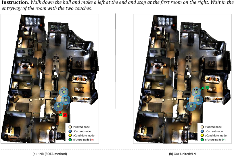
Visualization Example of Training.

To validate the effect of UnitedVLN for effective navigation in a continuous environment, we report the visualization comparison of navigation strategy between the baseline model (revised ETPNav) and Our UnitedVLN. Here, we also report each node navigation score for a better view, as shown in Figure 7. As shown in Figure 7, the baseline model achieves navigation error as obtains limited observations by relying on a pre-trained waypoint model [43] while our UnitedVLN achieves correct decision-marking of navigation by obtaining full future explorations by aggregating intuitive appearances and complicated semantics information. In addition, we also visualize a comparison of navigation strategy between the HNR [115] (SOTA method) and Our UnitedVLN. Compared to HNR relying on limited future features, our UnitedVLN instead aggregates intuitive appearances and complicated semantics information for decision-making and achieving correct navigation. This proves the effect of RGB-united-feature future representations, improving the performance of VLN-CE.