Unitary Approximate Message Passing for Matrix Factorization
Abstract
We consider matrix factorization (MF) with certain constraints, which finds wide applications in various areas. Leveraging variational inference (VI) and unitary approximate message passing (UAMP), we develop a Bayesian approach to MF with an efficient message passing implementation, called UAMP-MF. With proper priors imposed on the factor matrices, UAMP-MF can be used to solve many problems that can be formulated as MF, such as non-negative matrix factorization, dictionary learning, compressive sensing with matrix uncertainty, robust principal component analysis, and sparse matrix factorization. Extensive numerical examples are provided to show that UAMP-MF significantly outperforms state-of-the-art algorithms in terms of recovery accuracy, robustness and computational complexity.
Index Terms:
Variational inference (VI), approximate message passing (AMP), matrix factorization (MF), compressive sensing (CS), dictionary learning (DL), robust principal component analysis (RPCA).I Introduction
We consider the problem of matrix factorization (MF) with the following model
| (1) |
where denotes a known (observation) matrix, accounts for unknown perturbations or measurement errors, and the matrices and are two factor matrices to be obtained. Depending on concrete application scenarios, the MF problem in (1) often has specific requirements on the matrices and . For example, in non-negative matrix factorization (NMF) [1], the entries of and need to take non-negative values. In dictionary learning (DL) [2], matrix is sparse matrix and is a dictionary matrix to be learned. In compressive sensing with matrix uncertainty (CSMU) [3], is sparse and the sensing matrix can be modeled as , where the matrix is known, and denotes an unknown perturbation matrix. The robust principal component analysis (RPCA) problem [4] can also be formulated as (1), where both and admit specific structures [5]. We may also be interested in sparse MF, where both matrices and are sparse.
Many algorithms have been developed to solve the above problems. For NMF, the multiplication (Mult) update algorithm proposed in [6] is often used, which is simple to implement, and produces good results. The alternating least squares (ALS) algorithm was proposed in [7] for NMF, where two least squares steps are performed alternately. The above two algorithms are very popular and are built in the MATLAB library. The projected gradient descent (AlsPGrad) [8] algorithm, which is an improvement to Mult, usually has faster convergence speed. To solve the DL problem, one can use algorithms such as K-SVD (singular value decomposition) [9] and SPAMS (sparse modeling software) [10]. K-SVD is often effective, but can be trapped in local minima or even saddle points. The SPAMS algorithm often does not perform well when the number of training samples is small. For CSMU, the sparsity-cognizant total least squares (S-TLS) method was developed in [11] by extending the classical TLS approach. For the RPCA problem, many algorithms have been proposed. The work in [4] developed iterative thresholding algorithms with low complexity, but their convergence is usually slow. The inexact augmented Lagrange multiplier algorithm (IALM) [12] and low-rank matrix fitting algorithm (LMaFit) [13] deliver better convergence speed and performance.
Another line of techniques is based on the Bayesian framework, especially with the approximate message passing (AMP) algorithm [14], [15] and its extension or variants. With Bayesian approaches, the requirements on matrices and for the factorization in (1) are incorporated by imposing proper priors on them. The AMP algorithm is employed due to its low complexity. AMP was originally developed for compressive sensing based on loopy belief propagation (BP) [14], and was later extended in [16] to solve the estimation problem with a generalized linear observation model. The bilinear generalized AMP (Bi-GAMP) algorithm was proposed in [5] to deal with the problem in (1). However, Bi-GAMP inherits the shortcoming of the AMP algorithm, i.e., it is not robust to generic matrices and . To achieve better robustness, a bilinear adaptive VAMP (BAd-VAMP) algorithm was proposed in [17] and generalized in [18]. However, for the general problem in (1), to reduce computational complexity, BAd-VAMP does not allow the use of priors for matrix , i.e., it is treated as a deterministic unknown matrix. This makes BAd-VAMP incapable of dealing with the requirements on , e.g., RPCA or sparse MF where should be sparse. In addition, there is still considerable room for improvement in terms of performance, robustness and computational complexity. In [19], with UAMP [20] (which was formally called UTAMP), a more robust and faster approximate inference algorithm (called Bi-UTAMP in [19]) was proposed, which is designed for specially structured in (1), i.e., , where matrices are known, and coefficients (and matrix ) need to be estimated.
In this work, with the framework of variational inference (VI) [21], we develop a more efficient Bayesian algorithm leveraging UAMP. The use of VI requires the updates of two vairational distributions on and , which may be difficult and expensive With matrix normal distributions [22] and through a covariance matrix whitening process, we incorporate UAMP into VI to deal with the updates of the variational distributions. The VI-based method is implemented using message passing with UAMP as its key component, leading to an algorithm called UAMP-MF. Inheriting the low complexity and robustness of UAMP, UAMP-MF is highly efficient and robust. It has cubic complexity per iteration, which is considered low for an MF problem (note that even the multiplication of two matrices has cubic complexity). Enjoying the flexibility of a Bayesian approach, UAMP-MF is able to handle various problems in a unified way with different priors. We focus on its applications to NMF, DL, CSMU, RPCA and sparse MF, and compare its performance with various algorithms, including IAML, LMaFit and Bi-GAMP for RPCA, K-SVD, SPAMS and BAd-VAMP for DL, BAd-VAMP for the CSMU, AlsPGrad, and Mult for NMF. Extensive numerical results are provided to demonstrate the superiority of UAMP-MF in terms of recovery performance, robustness and computational complexity.
The remainder of this paper is organized as follows. In Section II, VI, (U)AMP and matrix normal distribution are briefly introduced. The UAMP-MF algorithm is derived in Section III. Applications of UAMP-MF to NMF, RPCA, DL, CSMU and sparse MF are investigated in Section IV, followed by conclusions in Section V.
Throughout the paper, we use the following notations. Boldface lower-case and upper-case letters denote vectors and matrices, respectively, and superscript represents the transpose operation. A Gaussian distribution of with mean and variance is represented by . Notation denotes the trace operation. The relation for some positive constant is written as . The operation returns a diagonal matrix with on its diagonal. We use and to represent the element-wise product and division between and , respectively. We use to denote element-wise magnitude squared operation for , and is the Frobenius norm of . The notations 1, 0 and denote an all-one matrix, an all-zero matrix and an identity matrix with a proper size, respectively. The above operations defined for matrices can also be applied to vectors. We use to denote the vectorization operation.
II Preliminaries
II-A Variational Inference
VI is a machine learning method widely used to approximate posterior densities for Bayesian models [21], [23]. Let and be the set of hidden (latent) variables and visible (observed) variables, respectively, with joint distribution . The goal of VI is to find a tractable variational distribution that approximates the true posterior distribution . With the distribution , the log marginal distribution of the observed variables admits the following decomposition
| (2) |
where the variational lower bound is given as
| (3) |
and the Kullback-Leibler (KL) divergence between and is
| (4) |
The distribution that minimizes the KL divergence can be found by maximizing the variational lower bound .
VI can be implemented with message passing with the assistance of graphical models such as factor graphs. If the variational distribution with some factorization is chosen, e.g.,
| (5) |
where , then the variational distribution may be found through an iterative procedure [21] with the update rule
| (6) |
Here is a local factor associated with and , depending on the structure of the factor graph. The update of is carried out iteratively until it converges or a pre-set number of iterations is reached.
II-B (U)AMP
AMP was derived based on loopy BP with Gaussian and Taylor-series approximations [24], [16], which can be used to recover from the noisy measurement with being a zero-mean white Gaussian noise vector. AMP works well with an i.i.d. Gaussian , but it can easily diverge for generic [25]. Inspired by [26], the work in [20] showed that the robustness of AMP can be remarkably improved through simple pre-processing, i.e., performing a unitary transformation to the original linear model [19]. As any matrix has an SVD with and being two unitary matrices, performing a unitary transformation with leads to the following model
| (7) |
where , , is an rectangular diagonal matrix, and remains a zero-mean white Gaussian noise vector with the same covariance as .
Applying the vector step size AMP [16] with model (7) leads to the first version of UAMP (called UAMPv1) shown in Algorithm 1. Note that by replacing and with and in Algorithm 1, the original AMP algorithm is recovered. An average operation can be applied to two vectors: in Line 7 and in Line 5 of UAMPv1 in Algorithm 1, leading to the second version of UAMP [20] (called UAMPv2), where the operations in the brackets of Lines 1, 5 and 7 are executed (refer to [19] for the detailed derivations). Compared to AMP and UAMPv1, UAMPv2 does not require matrix-vector multiplications in Lines 1 and 5, so that the number of matrix-vector products is reduced from 4 to 2 per iteration.
Initialize and . Set and . Define vector .
Repeat
Until terminated
In the (U)AMP algorithms, is related to the prior of and returns a column vector with th entry given by
| (8) |
where represents a prior for . The function returns a column vector and the th element is denoted by , where the derivative is taken with respect to .
II-C Matrix Normal Distribution
In this work, the matrix normal distribution is used in the derivation of VI for the MF problem, into which UAMP is incorporated, leading to the UAMP-MF algorithm. The matrix normal distribution is a generalization of the multivariate normal distribution to matrix-valued random variables [22]. The distribution of normal random matrix is
| (9) |
where is the mean of , and are the covariance among rows and columns of , respectively. The matrix normal distribution is related to the multivariate normal distribution in the following way
| (10) |
where and .
III Design of UAMP-MF
The Bayesian treatment of the MF problem leads to great flexibility. Imposing proper priors and on and , we can accommodate many concrete MF problems. For example in DL, we aim to find sparse coding of data set , where is the dictionary and is the sparse representation with the dictionary. For the entries of , we can use a Gaussian prior
| (11) |
while for the entries of , we can consider a sparsity promoting hierarchical Gaussian-Gamma prior
| (12) | |||||
| (13) |
In Section IV, more examples on the priors, including NMF, RPCA, CSMU and sparse MF, are provided.
With the priors and model (1), if the a posteriori distributions and can be found, then the estimates of and are obtained, e.g., using the a posteriori means of and to serve as their estimates. However, it is intractable to find the exact a posteriori distributions in general, so we resort to the approximate inference method VI to find their variational approximations and . Finding the varational distributions are still challenging due to the large dimensions of and , and the priors of and may also lead to intractable and . In this work, through a covariance matrix (model noise) whitening process, UAMP is incorporated to solve these challenges with high efficiency. This also leads to Gaussian variational distributions and , so that the estimates of and (i.e., the a posteriori means of and ) appear as the parameters of the variational distributions.
Leveraging UAMP, we carry out VI in a message passing manner, with the aid of a factor graph representation of the problem. This leads to the message passing algorithm UAMP-MF. In the derivation of UAMP-MF, we use the notation to denote a message passed from node to node , which is a function of . The algorithm UAMP-MF is shown in Algorithm 2, which we will frequently refer to in this section.
III-A Factor Graph Representation
Initialization: , , , . , , , . Repeat
Until terminated
With model (1), we have the following joint conditional distribution and its factorization
| (14) | |||||
where
| (15) | |||||
The precision of the noise has an improper prior [27], and the priors for and denoted by and are customized according to the requirements in a specific problem. The factor graph representation of is depicted in Fig.1, where the arguments of the local functions are dropped for the sake of conciseness. We define a variational distribution
| (16) |
and we expect that , and . Next, we study how to efficiently update , and iteratively.

III-B Update of
According to VI, with and (updated in the previous iteration), we update . As shown by the factor graph in Fig. 1, we need to compute the message from the factor node to the variable node and then combine it with the prior . Later we will see that is a matrix normal distribution, i.e., with , and is a Gamma distribution. It turns out that the message is matrix normal, as shown by Proposition 1.
Proposition 1: The message from to is a matrix normal distribution of , which can be expressed as
| (17) |
with
| (18) |
| (19) |
and
| (20) |
The computation of is shown in (46).
Proof.
See Appendix A. ∎
According to VI, this message is combined with the prior to obtain . This can be challenging as may lead to an intractable and high computational complexity. Next, leveraging UAMP, we update efficiently. It is also worth mentioning that, with the use of UAMP, the matrix inversion involved in (19) does not need to be performed.
Note that and . The result in (17) indicates that . This leads to the following pseudo observation model
| (21) |
where , i.e., the model noise is not white. We can whiten the noise by left-multiplying both sides of (21) by , leading to
| (22) |
where is white and Gaussian with covariance . Through the whitening process, we get a standard linear model with white additive Gaussian noise, which facilitates the use of UAMP. Considering all the vectors in , we have
| (23) |
where is white and Gaussian.
With model (23) and the prior , we use UAMP to update . Following UAMP, a unitary transformation needs to be performed with the unitary matrix obtained from the SVD of (or eigenvalue decomposition (EVD) as the matrix is definite and symmetric), i.e.,
| (24) |
with being a diagonal matrix. After performing the unitary transformation, we have
| (25) |
where , and , which is still white and Gaussian.
From the above, it seems costly to obtain and in model (25). Specifically, a matrix inverse operation needs to be performed according to (19) so that in (18) can be obtained; a matrix squared root operation is needed to obtain ; and an SVD operation is required to . Next, we show that the computations can be greatly simplified.
Instead of computing and followed by SVD of , we perform EVD to , i.e.,
| (26) |
where the diagonal matrix
| (27) |
Hence , where the computation of is trivial as is a diagonal matrix. Meanwhile, the computation of the pseudo observation matrix can also be simplified:
| (28) | |||||
For convenience, we rewrite the unitary transformed pseudo observation model as
| (29) |
The above leads to Lines 1-3 of UAMP-MF in Algorithm 2.
Due to the prior , the use of exact often makes the message update intractable. Following UAMP in Algorithm 1, we project it to be Gaussian, which can also be interpreted as performing the minimum mean squared estimation (MMSE) based on the pseudo observation model (29) with prior . These correspond to Lines 4-11 of UAMP-MF in Algorithm 2. We assume that the prior are separable, i.e., , then the operations in Lines 10 and 11 are element-wise as explained in the following. As the estimation is decoupled by (U)AMP, we assume the following scalar pseudo models
| (30) |
where is the th element of in Line 9 of the UAMP-MF algorithm, represents a Gaussian noise with mean zero and variance , and is the th element of in Line 8 of the UAMP-MF algorithm. This is significant as the complex estimation is simplified to much simpler MMSE estimation based on a number of scalar models (30) with prior . With the notations in Lines 10 and 11, for each entry in , the MMSE estimation leads to a Gaussian distribution
| (31) |
where and is the th element of in Line 11 and the th element of in Line 10, respectively. We can see that each element has its own variance. To facilitate subsequent processing, we make an approximation by assuming that the elements of each row in have the same variance, which is the average of their variances. Then they are collectively characterized by a matrix normal distribution, i.e., with and , where represents the average operation on the rows of . This leads to Line 12 of UAMP-MF in algorithm 2.
III-C Update of
With the updated and , we compute the message from to according to VI. Regarding the message, we have the following result.
Proposition 2: The message from to is a matrix normal distribution about , which can be expressed as
| (32) |
with
| (33) |
and
| (34) |
where .
Proof.
See Appendix B. ∎
Then we combine the message with the prior of to update . This will also be realized with UAMP through a whitening process. The procedure is similar to that for , and the difference is that the pseudo model is established row by row (rather than column by column) by considering the form of .
With the message and
| (35) |
where is the th row vector, we have the pseudo observation model
| (36) |
where . Whitening operation to (36) leads to
| (37) |
where , which is white and Gaussian with covariance . Collecting all rows and representing them in matrix form, we have
| (38) |
UAMP is then employed with the model (38). Using the ideas in the previous section for updating , we obtain the unitary transformed model efficiently.
We first perform an EVD to matrix , i.e.,
| (39) |
Then the unitary transformed model is given as
| (40) |
where
| (41) | |||||
| (42) |
and is white and Gaussian. The above leads to Lines 13-15 of UAMP-MF in Algorithm 2.
Following UAMP in Algorithm 1, we obtain and project it to be Gaussian, which correspond to Lines 16-23 of UAMP-MF Algorithm 2. Similar to the case for updating , to accommodate with a matrix normal distribution, we make an approximation by assuming the entries in each column of share a common variance, which is the average of their variances. Then with and (i.e., Line 24 of UAMP-MF in Algorithm 2), where represents the average operation on the columns of .
III-D Update of
With and , we update , i.e., combining the message from to and its prior .
Proposition 3: The message from to can be expressed as
| (43) |
where
| (44) |
Proof.
See Appendix C. ∎
With the message and the prior , can be computed as
| (45) |
which is a Gamma distribution. Then the mean of is obtained as
| (46) |
which is Line 25 of UAMP-MF.
III-E Discussion and Computational Complexity
Regarding UAMP-MF in Algorithm 2, we have the following remarks:
-
•
We do not specify the priors of and in Algorithm 2. The detailed implementations of Lines 10, 11, 22 and 23 of the algorithm depends on the priors in a concrete scenario. Various examples are provided in Section IV.
-
•
As the MF problem often has local minima, we can use the strategy of restart to mitigate the issue of being stuck at local minima. In addition, the iterative process can be terminated based on some criterion, e.g., the normalized difference between the estimates of two consecutive iterations is smaller than a threshold.
-
•
There are often hyper-parameters in the priors of and . If we do not have knowledge on these hyper-parameters, their values need to be leaned or tuned automatically. Thanks to the factor graph and message passing frame work, these extra tasks can be implemented by extending the factor graph in Fig. 1.
In the following, we show how to learn the hyper-parameters of the prior of . We assume that is sparse and the sparsity rate is unknown. In this case, we may employ the sparsity promoting hierarchical Gaussian-Gamma prior [27]. The prior is then , where and with and being the shape parameter and scale parameter of the Gamma distribution, respectively. While the precision is to be learned, the values for and are often set empirically, e.g., [27]. It is worth mentioning that can be tuned automatically to improve the performance [28].
The factor graph representation for this part is shown in Fig. 2. Also note that UAMP decouples the estimation as shown by the pseudo model (30), indicating that the incoming message to the factor graph in Fig. 2 is Gaussian, i.e.,
| (47) |
We perform inference on and , which can also be achieved by using VI with a variational distribution .
According to VI,
| (48) | |||||
with shown in (52), and
| (49) |
The message can be expressed as
| (50) | |||||
The message is the predefined Gamma distribution, i.e., . According to VI,
| (51) | |||||
Thus
| (52) | |||||
where
| (53) |
The above computations for all the entries of can be collectively expressed as
| (54) | |||
| (55) | |||
| (56) |
where is a matrix with as its entries.
We see that UAMP-MF in Algorithm 2 involves matrix multiplications and two EVDs per iteration, which dominate its complexity. The complexity of the algorithm is therefore in a cubic order, which is low in a MF problem (the complexity of two matrices product is cubic). In the next section, we will compare the proposed algorithm with state-of-the-art methods in various scenarios. As the algorithms have different computational complexity per iteration and the numbers of iterations required for convergence are also different, we will compare their complexity in terms of runtime, as in the literature. Extensive examples show that UAMP-MF is much faster than state-of-the-art algorithms in many scenarios, and often delivers significantly better performance.
IV Applications and Numerical Results
We focus on the applications of UAMP-MF to NFM, RPCA, DL, CSMU and sparse MF. Extensive comparisons with state-of-the-art algorithms are provided to demonstrate its merits in terms of robustness, recovery accuracy and complexity.
IV-A UAMP-MF for Robust Principal Components Analysis
In RPCA [4], we aim to estimate a low-rank matrix observed in the presence of noise and outliers. The signal model for RPCA can be written as
| (57) |
where the product of a tall matrix and wide matrix is a low-rank matrix, is a sparse outlier matrix, and is noise matrix, which is assumed to be Gaussian and white. To enable the use of UAMP-MF, the model (57) can be rewritten as [5]
| (58) |
which is a MF problem.
In (58), part of matrix is known, and part of matrix is sparse. These can be captured by imposing proper priors to the matrix entries. Similar to [5], for matrix , the priors are
| (59) |
where the entries corresponding to matrix have a zero variance, indicating that they are deterministic and known. For the sparse matrix , the sparsity rate is unknown, and we use the hierarchical Gaussian-Gamma priors. Then we have
| (60) |
where the precisions have Gamma distribution . If the knowledge about the parameter is unavailable, it can also be learned using VI, where the estimate of can be updated as with
| (61) | |||||
| (62) |
where and represent the upper () part of matrices and , and is the estimate of in the last round of iteration. In addition, the rank of matrix is normally unknown, and rank-selection can be performed using the method in [29].
We compare UAMP-MF with state-of-the-art algorithms including Bi-GAMP [5], IALM [12] and LMaFit [13]. The performance is evaluated in terms of the normalized mean squared error (NMSE) of matrix , which is defined as
| (63) |
In the numerical examples, the low rank matrix is generated from and with i.i.d standard Gaussian entries. The sparsity rate of matrix is denoted by , and the non-zero entries are independently drawn from a uniform distribution on , which are located uniformly at random in . It is noted that, with these settings, the magnitudes of the outliers and the entries of are on the same order, making the detection of the outliers challenging. The NMSE performance of various algorithms versus SNR is shown in Fig. 3, where , , and the rank and for (a), (b) and (c), respectively. It can be seen that IALM does not work well, and LMaFit struggles, delivering poor performance when and . Bi-GAMP and UAMP-MF deliver similar performance when , but when and , UAMP-MF still works very well while the performance of Bi-GAMP degrades significantly. We also show the performance of UAMP-MF with known rank , which is denoted by UAMP-MF(N) in Fig. 3, where we see that UAMP-MF has almost the same performance as UAMP-MF(N). Then, with , we vary the rank from 30 to 120 and the sparsity rate is changed from 0.05 to 0.3. The NMSE of the algorithms with different combinations of and is shown in Fig.4, where SNR = 60 dB. We see that the blue regions of UAMP-MF are significantly larger than other algorithms, indicating the superior performance of UAMP-MF.


Next we consider a more challenging case. All the settings are the same as the previous example except that the generated matrices and are no longer i.i.d., but correlated. Take as an example, which is generated with
| (64) |
where is an i.i.d Gaussian matrix, is an matrix with the th element given by where , and is generated in the same way but with size of . The parameter controls the correlation of matrix . Matrix is generated in the same way. We show the performance of the algorithms versus the correlation parameter in Fig. 5, where SNR = 60dB, the rank and in (a) and (b), respectively. The results show that UAMP-MF is much more robust and it outperforms other algorithms significantly when is relatively large.
The runtime of the algorithms is shown in Fig. 6, where the simulation parameter settings in Figs. 6 (a) and (b) are the same as those for Fig. 3(b) and Fig. 5(a), respectively. The results show that UAMP-MF can be much faster than Bi-GAMP while delivering better performance. IALM and LMaFit is faster than UAMP-MF, but they may suffer from severe performance degradation as shown in Figs. 3 - 5.
IV-B UAMP-MF for Dictionary Learning
In DL, we aim to find a dictionary that allows the training samples to be coded as
| (65) |
for some sparse matrix and some perturbation . To avoid over-fitting, a sufficiently large number of training examples are needed. For the entries of , we use the Gaussian prior as shown in (11), and for the entries of , we use the hierarchical Gaussian-Gamma prior (as we assume unknown sparsity rate) as shown in (12) and (13).


We compare UAMP-MF with the state-of-the-art algorithms including BAd-VAMP [17], K-SVD [9] and SPAMS [10]. It is worth mentioning that, in the case of DL, compared to Bi-GAMP, BAd-VAMP is significantly enhanced in terms of robustness and performance [17]. To test the robustness of the algorithms, we generate correlated matrix using (64) in the numerical examples. The sparse matrix is generated by selecting non-zero entries in each column uniformly and drawing their values from the standard Gaussian distribution, while all other entries are set to zero. The performance of DL is evaluated using the relative NMSE [17], defined as
| (66) |
where is a matrix accounting for the permutation and scale ambiguities.
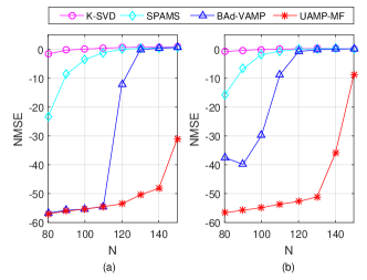

We first assume square dictionaries (i.e., ) and vary the values of and . The NMSE performance of the algorithms is shown in Fig.7, where SNR = 50dB. It can be seen that, when the correlation parameter , neither K-SVD nor SPAMS has satisfactory performance. In contrast, UAMP-MF and BAd-VAMP works well for a number of combinations of and , but the blue region of UAMP-MF is significantly larger than that of the BAd-VAMP. We show the performance of the algorithms versus the correlation parameter in Fig. 8, where , in (a) and in (b). It can be seen that UAMP-MF exhibits much higher robustness than other algorithms.
Next, we test the performance of the algorithms when learning an over-complete dictionary, i.e., . The setting for the experiments is same as those in the previous one, except that we fix and , but vary the value of . The NMSE of the algorithms is shown in Fig. 9, where and . The correlation parameter is set to in (a) and in (b). Again, K-SVD and SPAMS do not work well. Comparing BAd-VAMP with UAMP-MF, we see that UAMP-MF performs significantly better, especially when .
IV-C UAMP-MF for Compressive Sensing with Matrix Uncertainty
In practical applications of compressive sensing, we often do not know the measurement matrix perfectly, e.g., due to hardware imperfections and model mismatch. We aim to recover the sparse signal (and estimate the measurement matrix ) from the noisy measurements with
| (67) |
where is a known matrix and is an unknown disturbance matrix. Compared to the case of DL, the difference lies in the prior of . We assume that the entries of are modeled as i.i.d Gaussian distributed variables, i.e., , so the prior of can be represented as . For the entries of , we still use the hierarchical Gaussian-Gamma prior. It is worth noting that, if the sparsity of exhibits some pattern, e.g., the columns of share a common support, we can impose that the entries of each row of share a common precision in their Gaussian priors to capture the common support.


In the numerical example, to test the robustness of the algorithms, we generate correlated matrices and using (64). The sparse matrix is generated in the same way as before. It is noted that, different from DL, the ambiguity does not exist thanks to the known matrix . The performance is evaluated using the NMSE of
| (68) |
The NMSE performance of UAMP-MF and BAd-VAMP is shown in Fig.11 and Fig. 12 for various combinations of and . The parameter and in Figs. 11 and 12, respectively and SNR = 50dB. It can be seen that, UAMP-MF outperforms BAd-VAMP significantly when the correlation coefficient . The runtime comparison is shown in Fig. 13, which indicate that UAMP-MF is much faster.
IV-D UAMP-MF for Non-Negative Matrix Factorization
The NMF problem [1] finds various applications [30], [31]. In NMF, from the observation
| (69) |
where , we aim to find a factorization of as the product of two non-negative matrices and , i.e., . To achieve NMF with UAMP-MF, we set the priors of and to be i.i.d non-negative Gaussian, i.e.,
| (70) | |||
| (71) |
where is the complementary cumulative distribution function.


We compare UAMP-MF with the alternating non-negative least squares projected gradient algorithm (AlsPGrad) [8] and multiplicative update algorithm (Mult)[7]. In the numerical examples, we set and . The metric used to evaluate the performance is defined as
| (72) |
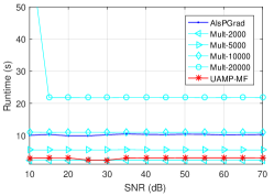
For Mult, we use the built-in function ‘nnmf’ in Matlab, and the termination tolerance is set to and maximum number of iterations is set to 2000, 5000, 10000 and 20000 for comparison.
The NMSE results are shown in Fig. 14 and the runtime is shown in Fig. 15. It can be seen that, with the increase of the maximum number of iterations, the performance of Mult improves considerably, but it comes at the cost of significant increase in runtime. AlsPGrad delivers performance similar to that of Mult with 20000 iterations. UAMP-MF delivers the best performance while with significant smaller runtime compared to Mult (except Mult-2000) and AlsPGrad.


IV-E UAMP-MF for Sparse Matrix Factorization
We consider the use of UAMP-MF to solve the sparse MF problem [32]. From the observation
| (73) |
where , and we aim to find a factorization of as the product of two sparse matrices and , i.e., .
To find the sparse matrices and with UAMP-MF, we use the sparsity promoting hierarchical Gaussian-Gamma prior for entries in both matrices, i.e.,
| (74) | |||||
| (75) | |||||
| (76) | |||||
| (77) |
The computations of the a posterior means and variances of the entries of and are the same as (54)-(56). We compare the performance of UAMP-MF and BAd-VAMP, and the results are shown in Fig.16 for various combinations of and , where , SNR = 50dB, and the sparsity rate of and is set to . It can be seen that the performance of UAMP-MF is significantly better than that of BAd-VAMP as no priors can be imposed on in BAd-VAMP.
We can also achieve sparse NMF with UAMP-MF, where and a sparse non-negative factorization is to be found. In this case, we can employ a non-negative Bernoulli-Gaussian distribution for the entries in both and . We compare UMAP-MF with Mult and AlsPGrad and the numerical results are shown in Fig. 17, where the sparsity rate for both and , , and . We can see that the performance of UAMP-MF is much better than that of other algorithms as they lack a sparsity promoting mechanism.
The runtime comparisons for sparse MF and spares NMF are shown in Fig. 18. It can be seen that UAMP-MF is much faster than BAd-VAMP. Compared to AlsGrad and Mul with 2000 iterations, UAMP-MF has similar runtime but delivers much better performance.
V Conclusions
In this paper, leveraging variational inference and UAMP, we designed a message passing algorithm UAMP-MF to deal with matrix factorization, where UAMP is incorporated into variational inference through a whitening process. By imposing proper priors, UAMP-MF can be used to solve various problems, such as RPCA, DL, CSMU, NMF, sparse MF and sparse NMF. Extensive numerical results demonstrate the superiority of UAMP-MF in recovery accuracy, robustness, and computational complexity, compared to state-of-the-art algorithms.
Appendix A Proof of Proposition 1
According to VI, the message from to can be expressed as
| (78) | |||
| (79) |
where , and . In the derivation of (78), we use the matrix identity [33].
Appendix B Proof of Proposition 2
According to VI, the message is computed as
| (87) |
where . Similar to the derivation of (83), the integration of the terms in (87) can be expressed as
| (88) |
and
| (89) |
The message from to can be represented as
| (90) |
Comparing the above against the matrix normal distribution, we obtain the result shown by (32) - (34).
Appendix C Proof of Proposition 3
References
- [1] D. D. Lee, “Learning parts of objects by non-negative matrix factorization,” Letter of Nature, vol. 401, pp. 788–791, 1999.
- [2] R. Rubinstein, A. M. Bruckstein, and M. Elad, “Dictionaries for sparse representation modeling,” Proceedings of the IEEE, vol. 98, no. 6, pp. 1045–1057, June 2010.
- [3] H. Zhu, G. Leus, and G. B. Giannakis, “Sparsity-cognizant total least-squares for perturbed compressive sampling,” IEEE Transactions on Signal Processing, vol. 59, no. 5, pp. 2002–2016, May 2011.
- [4] E. J. Candes, X. Li, Y. Ma, and J. Wright, “Robust principal component analysis?” J. ACM, vol. 58, no. 3, Jun. 2011. [Online]. Available: https://doi.org/10.1145/1970392.1970395
- [5] J. T. Parker, P. Schniter, and V. Cevher, “Bilinear generalized approximate message passing—part i: Derivation,” IEEE Transactions on Signal Processing, vol. 62, no. 22, pp. 5839–5853, 2014.
- [6] D. D. Lee, “Algorithms for non-negative matrix factorization,” Advances in Neural Information Processing Systems, vol. 13, pp. 556–562, 2001.
- [7] M. W. Berry, M. Browne, A. N. Langville, V. P. Pauca, and R. J. Plemmons, “Algorithms and applications for approximate nonnegative matrix factorization,” Computational Statistics and Data Analysis, vol. 52, no. 1, pp. 155–173, 2007.
- [8] C.-J. Lin, “Projected gradient methods for nonnegative matrix factorization,” Neural Computation, vol. 19, no. 10, pp. 2756–2779, 2007.
- [9] M. Aharon, M. Elad, and A. Bruckstein, “K-SVD: An algorithm for designing overcomplete dictionaries for sparse representation,” IEEE Transactions on Signal Processing, vol. 54, no. 11, pp. 4311–4322, 2006.
- [10] J. Mairal, F. Bach, J. Ponce, and G. Sapiro, “Online learning for matrix factorization and sparse coding,” Journal of Machine Learning Research, vol. 11, pp. 19–60, 2010.
- [11] Zhu, Hao, Leus, Geert, Giannakis, Georgios, and B., “Sparsity-cognizant total least-squares for perturbed compressive sampling.” IEEE Transactions on Signal Processing, vol. 59, no. 5, pp. 2002–2016, 2011.
- [12] Z. Lin, M. Chen, and Y. Ma, “The augmented Lagrange multiplier method for exact recovery of corrupted low-rank matrices,” http://export.arxiv.org/abs/1009.5055, 2010.
- [13] Z. Wen, W. Yin, and Y. Zhang, “Solving a low-rank factorization model for matrix completion by a nonlinear successive over-relaxation algorithm,” Mathematical Programming Computation, vol. 4, no. 4, pp. 333–361, 2012.
- [14] D. L. Donoho, A. Maleki, and A. Montanari, “Message passing algorithms for compressed sensing: I. motivation and construction,” in 2010 IEEE Information Theory Workshop on Information Theory (ITW 2010, Cairo), Jan 2010, pp. 1–5.
- [15] ——, “Message passing algorithms for compressed sensing: II. analysis and validation,” in 2010 IEEE Information Theory Workshop on Information Theory (ITW 2010, Cairo), Jan 2010, pp. 1–5.
- [16] S. Rangan, “Generalized approximate message passing for estimation with random linear mixing,” in Proc. Int. Symp. Inf. Theory. IEEE, July. 2011, pp. 2168–2172.
- [17] S. Sarkar, A. K. Fletcher, S. Rangan, and P. Schniter, “Bilinear recovery using adaptive vector-amp,” IEEE Transactions on Signal Processing, vol. 67, no. 13, pp. 3383–3396, July 2019.
- [18] X. Meng and J. Zhu, “Bilinear adaptive generalized vector approximate message passing,” IEEE Access, vol. 7, pp. 4807–4815, 2019.
- [19] Z. Yuan, Q. Guo, and M. Luo, “Approximate message passing with unitary transformation for robust bilinear recovery,” IEEE Trans. Signal Process., vol. 69, pp. 617–630, Dec. 2020.
- [20] Q. Guo and J. Xi, “Approximate message passing with unitary transformation,” arXiv preprint arXiv:1504.04799, Apr. 2015.
- [21] J. Winn and C. M. Bishop, “Variational message passing,” J. Mach. Learn. Res., vol. 6, pp. 661–694, Apr. 2005.
- [22] D. J. De Waal, Matrix-Valued Distributions. Encyclopedia of Statistical Sciences, 1985.
- [23] M. I. Jordan, Z. Ghahramani, T. S. Jaakkola, and L. K. Saul, “An introduction to variational methods for graphical models,” Mach. Learn., vol. 37, no. 2, pp. 183–233, Nov. 1999.
- [24] D. L. Donoho, A. Maleki, and A. Montanari, “Message-passing algorithms for compressed sensing,” Proc. Nat. Acad. Sci., vol. 106, no. 45, pp. 18 914–18 919, Nov. 2009.
- [25] S. Rangan, P. Schniter, A. K. Fletcher, and S. Sarkar, “On the convergence of approximate message passing with arbitrary matrices,” IEEE Trans. Inf. Theory, vol. 65, no. 9, pp. 5339–5351, Sept. 2019.
- [26] Q. Guo, D. D. Huang, S. Nordholm, J. Xi, and Y. Yu, “Iterative frequency domain equalization with generalized approximate message passing,” IEEE Signal Process. Lett., vol. 20, no. 6, pp. 559–562, June. 2013.
- [27] M. E. Tipping, “Sparse bayesian learning and the relevance vector machine,” J. Mach. Learn. Res., vol. 1, p. 211–244, sep 2001. [Online]. Available: https://doi.org/10.1162/15324430152748236
- [28] M. Luo, Q. Guo, M. Jin, Y. C. Eldar, D. Huang, and X. Meng, “Unitary approximate message passing for sparse bayesian learning,” IEEE Transactions on Signal Processing, vol. 69, pp. 6023–6039, 2021.
- [29] J. T. Parker, P. Schniter, and V. Cevher, “Bilinear generalized approximate message passing Part ii: Applications,” IEEE Transactions on Signal Processing, vol. 62, no. 22, pp. 5854–5867, 2014.
- [30] J. M. Bioucas-Dias, A. Plaza, N. Dobigeon, M. Parente, Q. Du, P. Gader, and J. Chanussot, “Hyperspectral unmixing overview: Geometrical, statistical, and sparse regression-based approaches,” IEEE Journal of Selected Topics in Applied Earth Observations and Remote Sensing, vol. 5, no. 2, pp. 354–379, 2012.
- [31] W. Xu, “Document clustering based on non-negative matrix factorization,” Proceedings of SIGIR-03, 2003.
- [32] P. O. Hoyer, “Non-negative sparse coding,” in Neural Networks for Signal Processing, 2002. Proceedings of the 2002 12th IEEE Workshop on, 2002.
- [33] K. B. Petersen and M. S. Pedersen, The Matrix Cookbook. on-line, Sep. 2007, http://matrixcookbook.com.