UniKW-AT: Unified Keyword Spotting and Audio Tagging
Abstract
Within the audio research community and the industry, keyword spotting (KWS) and audio tagging (AT) are seen as two distinct tasks and research fields. However, from a technical point of view, both of these tasks are identical: they predict a label (keyword in KWS, sound event in AT) for some fixed-sized input audio segment. This work proposes UniKW-AT: An initial approach for jointly training both KWS and AT. UniKW-AT enhances the noise-robustness for KWS, while also being able to predict specific sound events and enabling conditional wake-ups on sound events. Our approach extends the AT pipeline with additional labels describing the presence of a keyword. Experiments are conducted on the Google Speech Commands V1 (GSCV1) and the balanced Audioset (AS) datasets. The proposed MobileNetV2 model achieves an accuracy of 97.53% on the GSCV1 dataset and an mAP of 33.4 on the AS evaluation set. Further, we show that significant noise-robustness gains can be observed on a real-world KWS dataset, greatly outperforming standard KWS approaches. Our study shows that KWS and AT can be merged into a single framework without significant performance degradation.
Index Terms: key-word spotting, audio tagging, convolutional neural networks, weakly supervised learning
1 Introduction
Keyword spotting (KWS) or wake word detection is nowadays a crucial front-end task for most intelligent voice assistants. When a user utters a specific key phrase, the keyword, an assistant wakes up and provides the user some service e.g., a weather report. Audio tagging (AT) is a task that aims to label a specific audio content into sound event classes e.g., a cat meowing or a dog barking. One of the current applications of AT models is the assistance of hearing-impaired people, to notify a user that some event inaudible to the user has happened e.g., a door has been knocked.
From a technical standpoint of view, KWS and AT are identical in their implementation. Specifically, given an input sample of some specific length e.g., 1 s, the goal of both tasks is to provide an output label signaling the presence of a keyword (KWS) or a sound event (AT). However, most real-world applications for these two tasks are exclusive: Either KWS or AT can be operational at a time.
This work proposes unified keyword audio tagging (UniKW-AT), which is capable of jointly modeling both tasks using a single model. The potential benefits of UniKW-AT are an improved robustness of a KWS model in regards to real-world noises, such as music, and the possibility to provide sound event information to the user. Additional benefits are the capability to incorporate different types of speech into the KWS post-processing, such as whispering or children’s speech.
Nonetheless, there are inherent problems when jointly training a single model for KWS and AT. First, training large-scale AT models utilizes weakly supervised training, since large-scale strongly labeled datasets are costly [1]. On the contrary, KWS models are commonly trained with strong supervision, where the keyword position in time is known. Second, AT models are trained with a multi-label objective, since multiple sound events can co-occur within some time segment, e.g., music playing in the background while people are talking. On the contrary, standard KWS models are commonly trained using a single-label objective such as categorical cross-entropy.
Our core contribution in this work is the first attempt at joint KWS and AT modeling, with a focus on a noise-robust KWS performance and sound event detection capability.
1.1 Previous work
Most previous work regarding KWS is focused on decreasing a model’s parameter size and increasing its inference speed [2]. Works such as [3, 4, 5] used convolutional neural networks (CNNs) for this matter, while more recently transformer based models [6, 7] and multi-layer perceptron (MLP) mixers [8, 9] have also received attention from the community.
On the other hand, works for AT generally are performance-oriented, meaning that few works exist that focus on practical implications of models such as inference time or model size. Similar to KWS research, CNNs dominate the research for AT, with notable examples being [10, 11]. Further, transformers have also been recently seen success [12, 13, 14]. However, previously introduced models in literature aimed at AT cannot be used for KWS, since KWS is an always-on feature computed on-device and previous work using CNN/Transformer models require a GPU for fast inference. Thus, our work focuses on the usage of lightweight and fast models.
2 Method
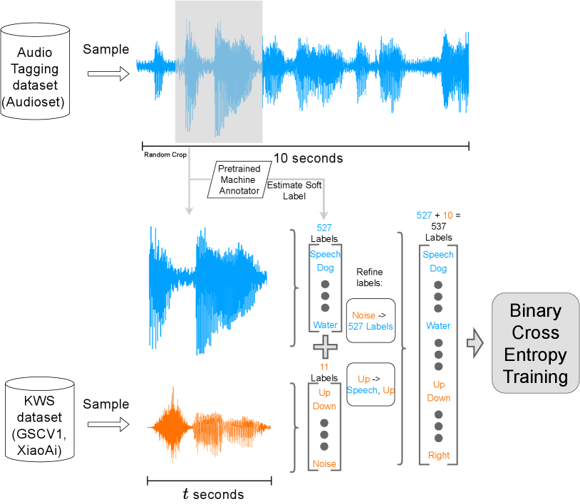
Our approach jointly models KWS and AT by treating KWS labels as additional target events within the standard AT training framework. Given the target KWS labelset with keywords and an AT labelset with sound events, we aim to model both tasks by merging both labelsets obtaining . Specifically, our method uses the sound event labels of Audioset (AS) [15] as . Models trained for KWS commonly contain a non-target label, also known as “noise” in their label set. In the case of UniKW-AT, this additional “noise” label is not needed, since most types of noise are already encompassed within the label set. Our approach first appends all target keywords to the available AS labels, resulting in target labels. All non-target keywords contained within a KWS dataset are mapped to the “Speech” label within .
Given a KWS dataset and an AT dataset, we preprocess the raw audio samples, such that the audio clip durations from both datasets match. Samples from both datasets are randomly cropped to some target duration i.e., 1 s. Randomly cropping the AT sample leads to a label misalignment problem, since labels are provided on a 10 s scale. This problem is partially solved by using a pre-trained machine annotator to create pseudo strong labels (PSL) [16] as the AT target.
We use the multi-label binary cross-entropy (BCE) objective in this work as our default training metric but provide comparisons to the standard cross-entropy (CE) objective in Section 4.2. We choose BCE in favor of CE due to its practical advantages during inference. For most real-world tasks, only a fraction of the provided sound event labels are relevant. In the case of BCE trained networks, undesirable labels (weights in the final linear layer) can be removed, since each label’s output probability is independent. This decreases model size, increases inference speed, and reduces power consumption while retaining performance for the labels of choice. The proposed framework is depicted in Figure 1.
3 Experiments
3.1 Datasets
Training
We make use of two training datasets being Google Speech Commands V1 (GSCV1) [17] and AS [15] in this work. GSCV1 contains 65,000 utterances of 30 different keywords, i.e., “Up”, “Right”, “Down”, spoken by thousands of people. We use the common 11 class subset of GSCV1, where the original 30 classes have been reduced to 10 common keywords: “Yes”, “No”, “Up”, “Down”, “Left”, “Right”, “On”, “Off”, “Stop”, “Go” while the rest 20 keywords are mapped to “unknown/noise”. The official training/validation/testing split containing 51,088/6,798/6,835 utterances, respectively, is used. Each sample within GSCV1 is at most 1 s long.
As for AT training, we use the 60 h long balanced subset of AS containing 21,292 audio clips with a duration of at most 10 s per clip.
Evaluation
Evaluation is split between the KWS and AT subtasks. AT evaluation uses the common evaluation subset of AS, containing 18,229 audio clips with an overall duration of 50 h.
KWS evaluation mainly focuses on the GSCV1 dataset, where 2,567 target keywords and 4,268 non-target samples are provided. Further, to explore the robustness of our approach across different domains, we additionally use three evaluation datasets for non-target evaluation, denoted as Eval-Neg. First, we remove English from the VoxLingua107 [18] dataset and use the leftover 106 languages for our out-domain evaluation denoted as VL106. We randomly sample 200 utterances from each of the 106 Languages, resulting in 21,200 utterances split into 209,240 one-second samples. Second, we use the Musan [19] dataset to test the noise-robustness of our approach.
| Dataset | Task | Purpose | # Samples |
|---|---|---|---|
| GSCV1 | KWS | Train | 51,088 (18 h) |
| GSCV1 | Eval | 6,835 (1.9 h) | |
| GSCV2 | Eval-Neg (In-domain) | 67,284 (18 h) | |
| Musan | Eval-Neg (Noise) | 394,432 (110 h) | |
| VL106 | Eval-Neg (Out-domain) | 209,240 (68 h) | |
| AS | AT | Train | 21,155 (58 h) |
| AS | Eval | 18,229 (50 h) |
Musan consists of 394,432 samples with music, speech, and babble noises. Third, we use the Google Speech Commands V2 (GSCV2) [17] dataset as our in-domain non-target evaluation dataset, where we remove all 10 target keywords and obtain 67,284 individual test samples. For all KWS evaluation datasets, we split all available audio clips into 1 s chunks, to match the training dataset duration. The datasets are summarized in Table 1.
3.2 Setup
Our work focuses on using a common MobileNetV2 [20] back-end as our default neural network due to its small parameter size of 2.9 M.
Regarding front-end feature extraction, all audio clips are converted to a 16 kHz sampling rate. We use log-Mel spectrograms (LMS) with 64 bins extracted every 10 ms with a window of 32ms. Batch-wise zero padding to the longest clip within a batch is applied for all experiments. Training runs with a batch size of 64 for at most 500 epochs using Adam optimization [21] with a starting learning rate of 0.001. During training, we use mean average precision (mAP) as our primary validation metric. The top-4 models achieving the highest mAP on the joint held-out validation dataset (GSCV1-valid and AS-balanced) are submitted for evaluation. The neural network back-end is implemented in Pytorch [22].
Assume that is an input feature of some length, the corresponding label, the trainable neural network, and the model prediction, i.e., . UniKW-AT is optimized using the binary cross entropy (BCE) objective defined as:
| (1) |
where can have multiple positive labels.
One of the core difficulties in jointly modeling KWS and AT are the differences in their training sample duration. In our experiments, the GSCV1 dataset contains only samples of duration less than s, while the majority of training samples in AS are of length 10 s. A simple merge of both datasets during training would lead to a large amount of padding (for the GSCV1 dataset). We provide an ablation study using the naïve data merging approach in Section 4.4.
3.3 Metrics
For KWS, we use accuracy as the default evaluation metric, while AT is mainly evaluated using mAP. Computing accuracy for the UniKW-AT approach requires the use of post-processing since the model can predict multiple labels at once. The core problem lies in the label ambiguity of speech-related labels since these are present for non-target and target keywords. For example, when presented with a target keyword, our approach will likely predict the tuple (speech, target-keyword), but in the case of a nontarget-keyword, our approach will only predict speech. Thus we compute the single-target output label as:
| (2) |
where is the raw model prediction vector, the predicted label index and a decision threshold. We optimized this threshold on the GSCV1 held-out validation dataset and obtained as our default choice. Finally, when evaluating on AS, we only output as the representative prediction vector.
4 Results
4.1 UniKW-AT
The results of our proposed UniKW-AT approach can be seen in Table 2. UniKW-AT achieves a comparable performance to other methods in regards to both AT and KWS. Notably, it outperforms the EfficientNet-B2 (15.70%), AST (14.80%), ResNet-50 (31.80%), and CNN14 (27.80%) methods on the balanced AS training set in regards to mAP performance (33.42%) without additional data augmentation or external pretraining. Further, our UniKW-AT method also contains the fewest parameters (2.9 M) within all investigated AT models.
Moreover, we observe that our approach only marginally lacks behind other models in terms of GSCV1 performance, achieving an accuracy of 97.53%, without further data augmentation. The much larger Wav2KWS [23] is the only approach to outperform UniKW-AT with an accuracy of 97.90%, while also containing 80 times more parameters. In addition, due to the benefits of the previously stated BCE training regime (see Section 2), we can remove the output layer’s weights and biases, stripping down the model size to 2.2M, denoted as “Ours-Strip”.
| Approach | #Params (M) | GSCV1 | AS |
|---|---|---|---|
| TC-ResNet8⋆ [5] | 0.06 | 96.10 | - |
| TC-ResNet14-1.5⋆ [5] | 0.3 | 96.60 | - |
| NAS1 [2] | 0.28 | 97.06 | - |
| NAS2 [2] | 0.88 | 97.22 | - |
| KWT-2⋆ [6] | 2.4 | 97.36 | - |
| KWT-3⋆ [6] | 5.3 | 97.24 | - |
| Wav2KWS⋆ [23] | 225 | 97.90 | - |
| MobileNetV2†⋆ [24] | 2.9 | - | 26.50 |
| EfficientNet-B0†⋆ [24] | 5.3 | - | 33.50 |
| EfficientNet-B2 [24] | 13.6 | - | 15.70 |
| EfficientNet-B2†⋆ [24] | 13.6 | - | 34.06 |
| ResNet-50†⋆ [24] | 25.6 | - | 31.80 |
| CNN14⋆ [10] | 76 | - | 27.80 |
| AST [12] | 87 | - | 14.80 |
| Ours-Strip | 2.2 | 97.53 | - |
| Ours | 2.9 | 97.53 | 33.42 |
We conclude that our results indicate that UniKW-AT provides excellent performance for both individual tasks.
4.2 Noise robustness
One of the benefits of the UniKW-AT approach is that it naturally enhances the noise robustness compared to standard KWS models. A core reason for this is the addition of AS into the training regime. Thus, we compare our proposed approach to a naïve CE trained baseline with the addition of AS as a noise source.
| Dataset | Baseline | Baseline w/AS | Ours |
|---|---|---|---|
| GSCV1 | 97.63 | 97.75 | 97.53 |
| GSCV2 | 97.47 | 98.90 | 98.90 |
| VL106 | 83.48 | 99.81 | 99.91 |
| Musan | 84.88 | 99.80 | 99.86 |
The results regarding noise-robustness are provided in Table 3. It can be seen that the naïve baseline performs well on in-domain evaluation, achieving an accuracy of 97.63% and 97.47% on the GSCV1 and GSCV2 evaluation sets, respectively. However, a significant performance drop is seen when evaluating the naïve baseline in out-domain (VL106) and noise (Musan) scenarios, since the baseline has been trained on clean data. When adding AS to the baseline training regime, performance steadily improves on all datasets compared to the baseline. With additional AS data the baseline approach slightly outperforms UniKW-AT on the clean GSCV1 evaluation set, achieving an accuracy of 97.75% against UniKW-AT’s 97.53%. On the other hand, the non-target keyword evaluation on all reported datasets (GSCV2, VL106, Musan) shows that our UniKW-AT method outperforms the baseline.
4.3 Real-world evaluation
In order to verify the effectiveness of the proposed approach, we explore its real-world usability. Here we use a private in-house dataset containing samples for our voice assistant “XiaoAi”. We collect 131 h of real-world training samples, split into 144,582 individual utterances with a length of 3 s. Within these 144,582 training samples, 100,582 (70%) contain the target keyword “XiaoAi Tongxue”. We evaluate our findings on two distinct datasets according to our evaluation framework (see Section 3.3). First, we use our “Common” dataset, containing 93,800 test utterances (80 h) with a balanced split of 50% positives (“XiaoAi Tongxue”) and negative samples. Second, we use a difficult non-target evaluation dataset, denoted as “Difficult”, which contains 3,731 (3 h) samples. The Difficult evaluation set consists of non-target keyword samples similar to the target keywords e.g., “Zhewei Tongxue” and other cases of false-alarms such as child babbling and vocalized music. Here we compare UniKW-AT against an in-house KWS model, denoted as “Base-Inhouse”.
| Dataset | Base-Inhouse | UniKW-AT (Ours) |
|---|---|---|
| Common | 99.98 | 99.85 |
| Difficult | 0 | 82.73 |
The results are displayed in Table 4. Real-world evaluation results show a similar trend to those in Table 3. The proposed UniKW-AT approach sightly underperforms on the Common evaluation set (99.85% vs. 99.98%), but significantly outperforms the baseline on the Difficult dataset (0% vs. 82.73%). These results show that UniKW-AT can enhance noise robustness in real-world KWS applications. Further performance gains can be achieved by tuning the decision threshold . For example, setting , one obtains 99.96% and 57.45% on the Common and Difficult test sets, respectively.
4.4 Ablations
In this section we explore the impact of two crucial components of our work: The PSL module and the effect of random cropping on the AT branch. The removal of random cropping, denoted as “ Crop” leads to zero padding samples from the KWS dataset to match the Audioset’s length i.e., 10 s. The removal of PSL uses the original hard labels provided in Audioset. The results of these ablation studies are displayed in Table 5.
| Method | GSCV1 | GSCV2 | VL106 | Musan | AS |
|---|---|---|---|---|---|
| Ours | 97.53 | 98.92 | 99.91 | 99.86 | 33.42 |
| Crop | 69.59 | 99.88 | 99.97 | 99.96 | 17.37 |
| PSL | 96.94 | 98.23 | 99.89 | 99.85 | 20.77 |
Impact of random cropping
It can be seen that random cropping of the AT branch has a profound impact on the KWS performance. Without it, the GSCV1 performance significantly degrades from 97.53% to 69.59% accuracy. Unsurprisingly, the performance on the three negative evaluation datasets improves, since the model rarely detects the presence of a keyword. Moreover, removing random cropping also results in the worst performance of 17.37% mAP on the AS evaluation set.
Impact of PSL
In line with the initial work for PSL [16], the performance on AS significantly improves (20.77% to 33.42%) by re-labeling the balanced AS training set. The results show that without PSL, performance uniformly degrades across all evaluation datasets. Surprisingly, the performance on the GSCV1 dataset improves with PSL from 96.94% to 97.53%.
5 Discussion
We would emphasize that our work is practically focused, such that we prefer lightweight models with an adequate performance over large models with excellent performance. Future work could focus on using more optimal models for this task since the proposed MobileNetV2 could be considered excessively large within the KWS community. Incidentally, compared to results within the AT community, our proposed MobileNetV2 framework is considered lightweight.
Even though this work indicates that UniKW-AT only marginally improves performance against common KWS baselines, it should be emphasized that UniKW-AT is a much more flexible framework for real-world KWS. One potential usage is to devise different post-processing approaches for different environments. For example, conditional KWS can be easily implemented i.e., wake-up only if children are speaking. Most importantly, we believe that UniKW-AT’s additional use case in form of AT would be justification enough to replace a pre-existing KWS model with UniKW-AT. Finally, it is noteworthy that UniKW-AT outperforms the commonly used YAMNet [25] model (30.6 vs. 33.4 mAP) for AT tasks with fewer parameters (3.7 M vs. 2.9 M).
6 Conclusions
This work proposes a novel approach to jointly modeling KWS and AT, denoted as UniKW-AT. Our approach models these two tasks as an extension of AT by using a single multi-label BCE training objective with a lightweight MobileNetV2 back-bone. UniKW-AT achieves an accuracy of 97.53% on the common GSCV1 benchmark dataset and an mAP of 33.4 on the Audioset evaluation subset, outperforming other works explicitly optimized for each respective task. Further, we provide results regarding noise-robustness using three out-of-domain scenarios and a study for real-world evaluation. For all three out-of-domain evaluation datasets, UniKW-AT shows superior performance to standard KWS models, rejecting up to 99.86% of noisy samples in the Musan dataset and 99.86% of samples in the VoxLingua106 dataset. Further, UniKW-AT also significantly enhances noise robustness against difficult samples in our real-world “XiaoAi” dataset, rejecting up to 82.73% of non-target samples. We believe that our work could spark future research for real-world applications of audio tagging and keyword spotting.
References
- [1] S. Hershey, D. P. W. Ellis, E. Fonseca, A. Jansen, C. Liu, R. Channing Moore, and M. Plakal, “The benefit of temporally-strong labels in audio event classification,” in ICASSP 2021 - 2021 IEEE International Conference on Acoustics, Speech and Signal Processing (ICASSP), 2021, pp. 366–370.
- [2] T. Mo, Y. Yu, M. Salameh, D. Niu, and S. Jui, “Neural Architecture Search for Keyword Spotting,” in Proc. Interspeech 2020, 2020, pp. 1982–1986. [Online]. Available: http://dx.doi.org/10.21437/Interspeech.2020-3132
- [3] T. N. Sainath and C. Parada, “Convolutional neural networks for small-footprint keyword spotting,” in Proc. Interspeech 2015, 2015, pp. 1478–1482.
- [4] B. Kim, S. Chang, J. Lee, and D. Sung, “Broadcasted Residual Learning for Efficient Keyword Spotting,” in Proc. Interspeech 2021, 2021, pp. 4538–4542.
- [5] S. Choi, S. Seo, B. Shin, H. Byun, M. Kersner, B. Kim, D. Kim, and S. Ha, “Temporal Convolution for Real-Time Keyword Spotting on Mobile Devices,” in Proc. Interspeech 2019, 2019, pp. 3372–3376.
- [6] A. Berg, M. O’Connor, and M. T. Cruz, “Keyword Transformer: A Self-Attention Model for Keyword Spotting,” in Proc. Interspeech 2021, 2021, pp. 4249–4253.
- [7] S. K. Sahu, S. Mitheran, J. Kamdar, and M. Gandhi, “Audiomer: A convolutional transformer for keyword spotting,” arXiv preprint arXiv:2109.10252, 2021.
- [8] M. M. Morshed and A. O. Ahsan, “Attention-free keyword spotting,” arXiv preprint arXiv:2110.07749, 2021.
- [9] D. Ng, Y. Chen, B. Tian, Q. Fu, and E. S. Chng, “Convmixer: Feature interactive convolution with curriculum learning for small footprint and noisy far-field keyword spotting,” arXiv preprint arXiv:2201.05863, 2022.
- [10] Q. Kong, Y. Cao, T. Iqbal, Y. Wang, W. Wang, and M. D. Plumbley, “PANNs: Large-Scale Pretrained Audio Neural Networks for Audio Pattern Recognition,” IEEE/ACM Transactions on Audio Speech and Language Processing, vol. 28, pp. 2880–2894, dec 2020.
- [11] E. Fonseca, X. Favory, J. Pons, F. Font, and X. Serra, “FSD50K: an open dataset of human-labeled sound events,” arXiv preprint arXiv:2010.00475, 2020.
- [12] Y. Gong, Y.-A. Chung, and J. Glass, “AST: Audio Spectrogram Transformer,” in Proc. Interspeech 2021, 2021, pp. 571–575.
- [13] K. Chen, X. Du, B. Zhu, Z. Ma, T. Berg-Kirkpatrick, and S. Dubnov, “Hts-at: A hierarchical token-semantic audio transformer for sound classification and detection,” arXiv preprint arXiv:2202.00874, 2022.
- [14] K. Koutini, J. Schlüter, H. Eghbal-zadeh, and G. Widmer, “Efficient training of audio transformers with patchout,” arXiv preprint arXiv:2110.05069, 2021.
- [15] J. F. Gemmeke, D. P. Ellis, D. Freedman, A. Jansen, W. Lawrence, R. C. Moore, M. Plakal, and M. Ritter, “Audio set: An ontology and human-labeled dataset for audio events,” in 2017 IEEE International Conference on Acoustics, Speech and Signal Processing (ICASSP). IEEE, 2017, pp. 776–780.
- [16] H. Dinkel, Z. Yan, Y. Wang, J. Zhang, and Y. Wang, “Pseudo strong labels for large scale weakly supervised audio tagging,” in ICASSP 2022 - 2022 IEEE International Conference on Acoustics, Speech and Signal Processing (ICASSP), 2022, pp. 336–340.
- [17] P. Warden, “Speech commands: A dataset for limited-vocabulary speech recognition,” arXiv preprint arXiv:1804.03209, 2018.
- [18] J. Valk and T. Alumäe, “VoxLingua107: a dataset for spoken language recognition,” in Proc. IEEE SLT Workshop, 2021.
- [19] D. Snyder, G. Chen, and D. Povey, “Musan: A music, speech, and noise corpus,” arXiv preprint arXiv:1510.08484, 2015.
- [20] M. Sandler, A. Howard, M. Zhu, A. Zhmoginov, and L.-C. Chen, “Mobilenetv2: Inverted residuals and linear bottlenecks,” in Proceedings of the IEEE conference on computer vision and pattern recognition, 2018, pp. 4510–4520.
- [21] D. P. Kingma and J. Ba, “Adam: A method for stochastic optimization,” arXiv preprint arXiv:1412.6980, 2014.
- [22] A. Paszke, S. Gross, F. Massa, A. Lerer, J. Bradbury, G. Chanan, T. Killeen, Z. Lin, N. Gimelshein, L. Antiga, A. Desmaison, A. Kopf, E. Yang, Z. DeVito, M. Raison, A. Tejani, S. Chilamkurthy, B. Steiner, L. Fang, J. Bai, and S. Chintala, “PyTorch: An Imperative Style, High-Performance Deep Learning Library,” in Advances in Neural Information Processing Systems 32, H. Wallach, H. Larochelle, A. Beygelzimer, F. Alché-Buc, E. Fox, and R. Garnett, Eds. Curran Associates, Inc., 2019, pp. 8026–8037.
- [23] D. Seo, H.-S. Oh, and Y. Jung, “Wav2kws: Transfer learning from speech representations for keyword spotting,” IEEE Access, vol. 9, pp. 80 682–80 691, 2021.
- [24] Y. Gong, Y.-A. Chung, and J. Glass, “Psla: Improving audio event classification with pretraining, sampling, labeling, and aggregation,” arXiv preprint arXiv:2102.01243, 2021.
- [25] M. Plakal and D. Ellis, “Yamnet,” 2022. [Online]. Available: https://github.com/tensorflow/models/blob/master/research/audioset/yamnet/README.md