Uniform Spanning Tree in Topological Polygons,
Partition Functions for SLE(8), and
Correlations in Logarithmic CFT
Abstract
We find explicit SLE() partition functions for the scaling limits of Peano curves in the uniform spanning tree (UST) in topological polygons with general boundary conditions. They are given in terms of Coulomb gas integral formulas, which can also be expressed in terms of determinants involving -periods of a hyperelliptic Riemann surface. We also identify the crossing probabilities for the UST Peano curves as ratios of these partition functions.
The partition functions are interpreted as correlation functions in a logarithmic conformal field theory (log-CFT) of central charge . Indeed, it is clear from our results that this theory is not a minimal model and exhibits logarithmic phenomena — the limit functions have logarithmic asymptotic behavior, that we calculate explicitly. General fusion rules for them could also be inferred from the explicit formulas. The discovered algebraic structure matches the known Virasoro staggered module classification, so in this sense, we give a direct probabilistic construction for correlation functions in a log-CFT of central charge describing the UST model.
Keywords:
(logarithmic) conformal field theory (CFT), correlation function, crossing probability, uniform spanning tree (UST), partition function, Schramm-Loewner evolution (SLE)
MSC: 82B20, 60J67, 60K35
1 Introduction
Random polymer models provide a plethora of interesting phenomena in statistical physics, probability theory, and related fields. For instance, many of them show features of criticality conjecturally related to conformal invariance. A particularly favorable setup for exact and rigorous results is the case of planar models. Indeed, one of the first examples where a conformal invariance result for a critical model was rigorously verified was the planar uniform spanning tree (UST): Lawler, Schramm & Werner showed [LSW04] that the random curve traversing along a uniformly chosen spanning tree (hereafter referred to as the UST Peano curve), which can also be thought of as a critical dense polymer, converges in the scaling limit to a Schramm-Loewner evolution process, with . In fact, the UST is quite a fruitful model, as it connects to other important models in various ways. For instance, the UST can be generated by loop-erased random walks via Wilson’s algorithm [Wil96], and the “branch-winding height functions” of the UST have the Gaussian free field as a scaling limit [Ken01]. This observation also leads to an analogue in the continuum: curves can be coupled with the Gaussian free field as flow lines [Dub09, MS17, BLR20]. However, even though substantial evidence for conformal invariance has been obtained for the UST model, there is still no clear conjecture on the full conformal field theory (CFT) describing its scaling limit.
In (heuristic) CFT parlance, the planar UST model should be described by some CFT with central charge , which remarkably is a non-unitary theory — unlike many well-known ones such as the Liouville CFT [KRV20] or the minimal model for the Ising model [CHI21]. In the non-unitary case there can even exist several theories with the same central charge and conformal weights. Physicists have proposed various descriptions for a theory (e.g., [Gur93, GK96, Kau00, PR07]), involving logarithmic fields. These are fields in the CFT with anomalous behavior, arising from the feature that the Virasoro dilation operator , which generates scalings of the physical space-time, is not diagonalizable (in particular, the Hamiltonian of the theory is not self-adjoint). This implies that the space of states has a complicated structure as a representation of the Virasoro algebra, containing non-trivial Jordan blocks for . They, in turn, result in logarithmic divergences in the correlation functions of the theory (cf. Section 1.4). We will show in the present work that the correlation functions have a clear probabilistic interpretation, which could be helpful in revealing the underlying complicated algebraic structures.
This article concerns a probabilistic model of UST Peano curves in (topological) polygons with various boundary conditions. We obtain scaling limit results expressed in terms of explicit quantities — determinantal expressions and Coulomb gas integrals. As a by-product of our results, we establish that any (boundary) CFT describing the UST model (once again, we say “any”, as there is no consensus for what the CFT should exactly be) must contain fields whose correlation functions have logarithmic divergences. Specifically, we show that the explicit scaling limit objects are conformally invariant or covariant, satisfy BPZ PDEs at level two, and we derive explicit fusion rules in terms of asymptotic behavior (with structure constants also determined), that manifestly show the emergence of a logarithmic CFT (log-CFT) structure. We believe that by providing (to our knowledge) the first mathematically rigorous probabilistic results towards a systematic log-CFT description of the scaling limit of the UST model, we also initiate the building of solid analytical foundations for such a theory, relevant in particular to random geometry and statistical physics.
1.1 Summary of main results
Let us summarize more precisely the main findings of the present work. We will consider uniformly chosen spanning trees on subsets of the square lattice, focusing on the behavior of the random chordal Peano curves between the tree and its dual. Specifically, we consider scaling limits of the UST model on polygons with an even number of marked boundary points. Thus, we fix and a polygon , that is, a bounded simply connected domain such that is locally connected, together with distinct marked boundary points in counterclockwise order. We encode boundary conditions in link patterns (i.e., planar/non-crossing pair partitions)
| (1.1) | ||||
where . For convenience, we have chosen a particular ordering of the endpoints of the links . We shall denote by the set of link patterns of links.
Our main results can be summarized as follows:
-
•
(Theorem 1.3): We identify the scaling limits of the UST Peano curves with any boundary condition . These are variants of the process, whose partition functions (denoted ) are determined by , arising naturally from the discrete holomorphic observable that we employ to derive this result. Let us remark that, compared to the earlier results [LSW04, Dub06, HLW24], the choice and analysis of the general observable is significantly more intricate, and the boundary conditions for it are non-trivial.
-
•
(Theorem 1.4): We find the scaling limits of all crossing probabilities of the UST Peano curves as ratios of and so-called pure partition functions (see [BBK05, Dub07, KL07, Pel19] and references therein for cases with ). In contrast to earlier lattice-level results [KW11], we obtain a more complete description of the scaling limits, provide explicit formulas in terms of integrals of Coulomb gas type, and interpret these probabilities in terms of operators in a log-CFT. Interestingly, the Coulomb gas integrals can also be written in terms of -periods of a suitable hyperelliptic Riemann surface (see Proposition 2.4) — in particular, they have a determinantal structure.
- •
Even though the log-CFT interpretation is rather heuristic, from the formal, algebraic viewpoint (in terms of the representation theory of the Virasoro algebra), we thus provide evidence that any CFT describing the planar UST model in the scaling limit must be a non-unitary, logarithmic CFT containing specific operator content (cf. Section 1.4). Our results furthermore provide a probabilistic construction for such a CFT in terms of correlation functions.
1.2 observables: Coulomb gas integrals and pure partition functions
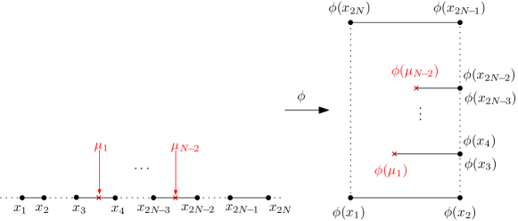
In order to state our scaling limit results, we first describe the objects that determine the scaling limit. We recommend readers only interested in the scaling limit results per se to first glance at Section 1.3 and then return to the present Section 1.2. However, let us point out that the results of the present section greatly differ from the previously considered cases of the critical Ising model () [Izy15, PW23], multiple LERW () [KW11, Kar20, KKP20], critical percolation () [Dub06], and critical random-cluster models () [Izy22, FPW24]. Indeed, when , for instance the pure partition functions can be uniquely classified as solutions to a certain PDE boundary value problem [FK15, PW19], whereas in the present case of , no classification is known and the techniques of [FK15, PW19] fail. Furthermore, while the Kac conformal weights and for in Equation (1.16) determine unambiguously the asymptotic boundary conditions for such a PDE boundary value problem, giving rise to two distinct Frobenius exponents, these exponents coincide when . This seemingly innocent property lies at the heart of the logarithmic phenomena in the CFT describing the scaling limit of the UST model.
For each as in (1.1), we define , where
to be a “Coulomb gas integral function” (for )
| (1.2) |
where the branch of the multivalued integrand is chosen to be real and positive when
and the integration in (1.2) is understood so that the integration variables avoid the ramification points by encircling them from the upper half-plane (see Section 2). With such a branch choice, actually takes values in , see Theorem 1.1. This fact is crucial for the probabilistic interpretation of these functions — however, it is not obvious.
Quite a specific feature to the present case of is that the function (1.2) also equals, up to a multiplicative factor, an integral of the Vandermonde determinant:
| (1.3) | ||||
is a matrix which can also be written in terms of -periods of a suitable hyperelliptic Riemann surface — see Proposition 2.4 and Equation (2.15, 2.16). Such a determinantal structure can be viewed as a feature of the fermionic nature of the UST model (CFT with ).
Historically, these Coulomb gas integrals stem from conformal field theory [DF84, Dub06, KP20], where they have been used as a general ansatz to find formulas for correlation functions. Specifically to our case, we seek correlation functions of so-called degenerate fields, which should satisfy a system of “BPZ PDEs” attributed to Belavin, Polyakov & Zamolodchikov [BPZ84],
| (PDE) |
and the specific covariance property
| (COV) |
for all Möbius maps of the upper half-plane such that .
Theorem 1.1.
The functions defined in (1.2) satisfy the PDE system (PDE), Möbius covariance (COV), and the following further properties.
-
(POS)
Positivity: For each and , we have , for all .
-
(ASY)
Asymptotics: With for the empty link pattern , the collection satisfies the following recursive asymptotics property. Fix and . Then, we have111Throughout, we use the cyclic indexing convention etc.
(-ASY1,1) (-ASY1,3) where
(1.4) and , and where denotes the link pattern obtained from by removing the link and relabeling the remaining indices by , and is the “tying operation” defined by
where (resp. ) is the pair of (resp. ) in (and are unordered).
-
(LIN)
Linear independence: The functions are linearly independent.
In short, the proof of Theorem 1.1 comprises Proposition 2.6, Proposition 2.8 (or Corollary 3.7), Proposition 2.9, Proposition 2.14, and the conclusion in Section 4.3.
-
•
The BPZ PDE system (PDE) can be verified by the following argument for the Coulomb gas integrals. The integration contours in (1.2) can be written as a closed surface in a suitable homology, and the integrand after being hit by the differential operator in (PDE) gives an exact form. Therefore, Stokes’ theorem can be used (with care) to argue that (1.2) is a solution to (PDE). We perform this argument in Proposition 2.8. The strategy is explained in detail in [KP20, Section 1]222The results in [KP20] concern the case of irrational values of , but the same idea for this part also works for rational ..
- •
-
•
In general, it is very difficult to establish positivity (POS) for Coulomb gas type integrals333For , positivity results have been established via a construction of partition functions explicitly in terms of probabilistic quantities, such as the Brownian loop measure and multiple [KL07, Law09, PW19, Wu20].. Once again, in our special case the positivity is guaranteed by the determinantal structure, see Proposition 2.14. This property is absolutely essential for the probabilistic interpretation and usage of for the scaling limit results stated below in Section 1.3; indeed, a priori are complicated complex valued functions expressed as iterated integrals (1.2).
-
•
Of the asymptotics properties in (ASY), the generic one, (-ASY1,1), is very easy to verify (Lemma 2.10), whereas the logarithmic one, (-ASY1,3), needs more detailed analysis (Lemma 2.11). These asymptotics properties are motivated by fusion rules in log-CFT, that in particular involve the logarithmic correction in one of the fusion channels. See Section 1.4 for discussion and literature.
-
•
Lastly, the linear independence of the functions is a consequence of their different asymptotic properties, as explained in the end of Section 4.3.
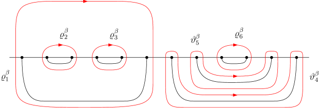
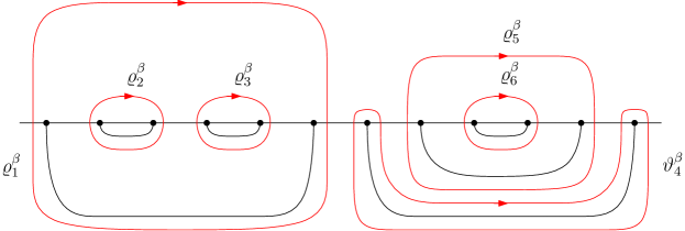
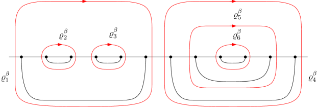
Theorem 1.1 shows that forms a basis for a solution space444It is not known to us what the dimension of the full solution space to the PDE system (PDE) is. However, it is plausible that imposing the additional constraint (COV) and possibly a bound for the growth of the solutions analogous to [FK15, Part 1, Eq. (20)], the dimension of the restricted solution space would equal the Catalan number . of the PDE system (PDE). There is another useful basis consisting of pure partition functions . To explain how these two bases are related, let us recall that a meander formed from two link patterns is the planar diagram obtained by placing and the horizontal reflection of on top of each other555Some authors call these “meandric systems.”:
| (1.5) |
We define the (renormalized, symmetric) meander matrix entries as
| (1.6) |
We also set by convention. By [DFGG97, Eq. (5.18)], the meander matrix (1.6) is invertible. We then define the pure partition functions as
| (1.7) |
Theorem 1.2.
The pure partition functions defined in (1.7) satisfy the PDE system (PDE), Möbius covariance (COV), and the following further properties.
-
(POS)
Positivity: For each and , we have , for all .
-
(ASY)
Asymptotics: With for the empty link pattern , the collection satisfies the following recursive asymptotics property. Fix and . Then, for all , using the notation (1.4), we have
(-ASY1,1) (-ASY1,3) -
(LIN)
Linear independence: The functions are linearly independent.
The proof of Theorem 1.2 comprises Lemmas 4.4 and 4.5 in Section 4, and the conclusion in Section 4.3. The proof also uses Theorem 1.1. The main difficulties are to prove the asymptotic properties (ASY) in Section 4.2, and the positivity (POS) in Section 4.3 — importantly, both use the fact that are related to UST crossing probabilities.
Generalizing the covariance property (COV), we extend the definitions of and to general polygons, whenever the derivatives of the associated conformal map in (COV) are defined. Thus, we set
and where is any conformal map from onto with , assuming that the marked boundary points lie on sufficiently regular boundary segments (e.g. for some ).
In general, a partition function (with ) will refer to a positive smooth function satisfying the BPZ PDE system (PDE) and Möbius covariance (COV). We can use any partition function to define a Loewner chain associated to : in the upper half-plane , started from , and with marked points , this is the Loewner chain driven by the solution to the stochastic differential equations (SDEs)
| (1.8) |
This process is well-defined up to the first time when either or is swallowed (i.e., when the denominator in the SDE (1.8) blows up). The functions and are examples of partition functions.
1.3 Scaling limit results: Uniform spanning tree in polygons
We now consider UST on a scaled square lattice (see the precise formulation in Section 3). Suppose that is a sequence of medial polygons on . A common notion of convergence for such a sequence is termed after Carathéodory (see Section 3.2). However, for our purposes, the following stronger notion of convergence phrased in terms of a curve metric is relevant. The set of planar oriented curves, that is, continuous mappings from to modulo reparameterization, is a complete and separable metric space
| (1.9) |
where the infimum is taken over all increasing homeomorphisms . We will assume that converges to a polygon in the following sense:
| (1.10) | ||||
where denotes the counterclockwise boundary arc between and . Note that such a convergence also implies convergence in the Carathéodory sense.
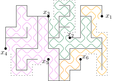
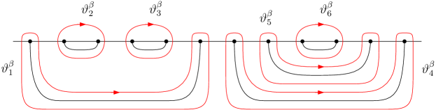
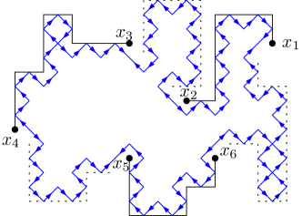
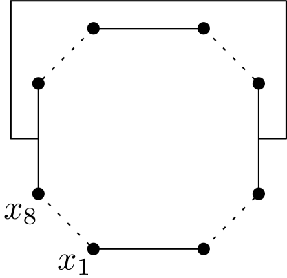
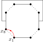
Next, let be the graph on the primal lattice corresponding to . Consider the primal polygon and spanning trees on it, with the following boundary conditions (see Figure 1.1): first, every other boundary arc is wired,
and second, these wired arcs are further wired together according to a non-crossing partition outside of . Note that there is a bijection between non-crossing partitions of the wired boundary arcs and planar link patterns with links, illustrated in Figure 3.2. Hence, we may encode the boundary condition by a label , and we thus speak of the UST with boundary condition (b.c.) . Let be a uniformly chosen spanning tree on with b.c. . Then, there exist curves on the medial lattice running along the tree and connecting pairwise. We call them UST Peano curves. The goal of this section is to describe the scaling limit of these Peano curves.
Our first result identifies the scaling limits of the UST Peano curves with type processes having specific partition functions, given exactly by the functions of Theorem 1.1, defined in (1.2). For , we have (cf. Lemma B.1) and the limit process in Theorem 1.3 is the chordal in between and [LSW04].
Theorem 1.3.
Fix a polygon whose boundary is a -Jordan curve. Fix also a link pattern . Suppose that a sequence of medial polygons converges to in the sense (1.10). Consider the UST on the primal polygon with boundary condition . For each , let be the Peano curve started from . Let be any conformal map from onto such that . Then, converges weakly to the image under of the Loewner chain with driving function solving the following SDEs, up to the first time when or is swallowed:
| (1.11) |
The main issue to prove Theorem 1.3 is to identify the limit and show its uniqueness. To this end, one can use a discrete holomorphic observable, which is natural when only one or two curves are present (in that case, there is at most one free parameter after fixing three parameters via conformal invariance). Dubédat proposed a formula for the simplest case of
| (1.12) |
in his article [Dub06] but without proof. His formula is different from ours at first sight, but it follows from Proposition 2.4 that they are actually the same. The recent work [HLW24] concerns the case of , which is solvable by an ordinary differential equation666H.W. learned the observable in [HLW24] from a master course delivered by S. Smirnov in 2015, but we are not able to identify a published reference.. However, the general involving non-trivial conformal moduli is significantly more difficult.
The proof of Theorem 1.3 is given in Section 3. Roughly, it follows the standard strategy: first, we need precompactness (tightness) of the family (from well-known arguments, cf. Lemma 3.1); second, we construct a discrete martingale observable (Sections 3.1–3.2); and third, we identify the subsequential limits through the observable (Section 3.4). The identification step involves deriving the expansion of the observable as approaches one of the marked points to a certain precision, and relating the expansion coefficients explicitly to the partition function (Lemmas 3.5 & 3.6 in Section 3.3). The observable from Proposition 3.4 also gives the scaling limit distribution of the loop-erased random walk branch in the UST, see [LW23].
Interestingly enough, the scaling limit of the observable (see Proposition 3.4) can be written, on the one hand, as an abelian integral (see Equation (3.10)),
| (1.13) |
involving the -periods discussed in Section 2,
and on the other hand, as a degenerate Schwarz-Christoffel conformal map (see Appendix C),
| (1.14) |
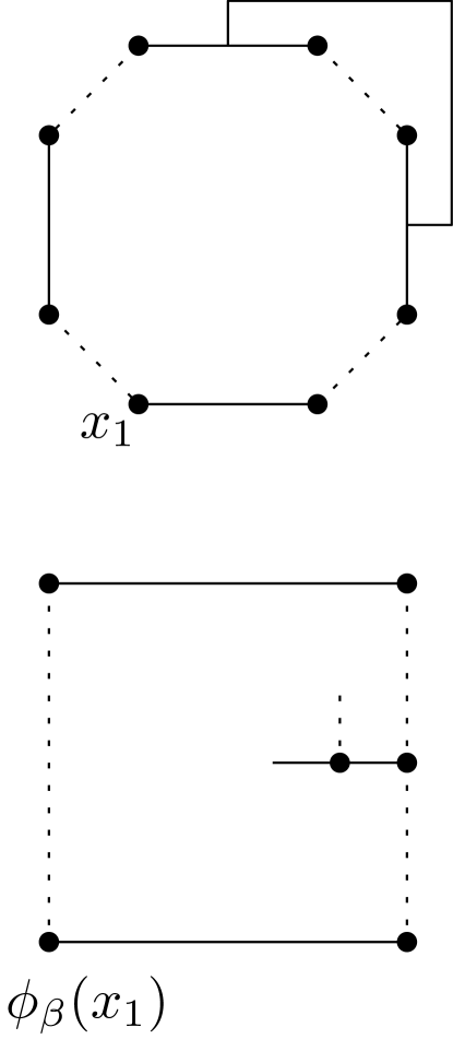
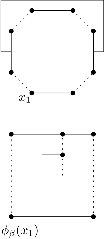
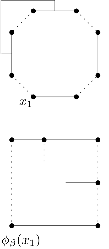
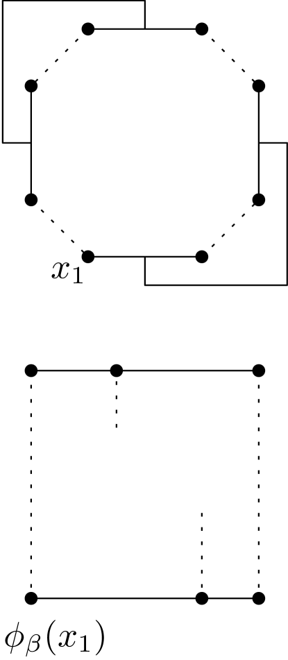
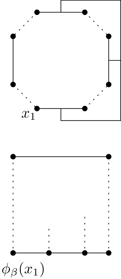
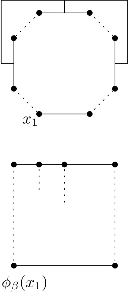
where the accessory parameters are mapped to the tips of the slits in the image of — see Figure 1.2 for an example.
In our second scaling limit result, we identify the scaling limits of the crossing probabilities of the Peano curves as ratios of pure partition functions with the partition functions , the latter arising from the choice of the boundary condition . Of course, the internal crossing pattern encoded in must be compatible with the b.c. , which is exactly what the meander matrix (1.6) ensures. We denote by the law of the UST with b.c. .
Theorem 1.4.
Let us briefly summarize the strategy for the proof of Theorem 1.4, given in detail in Sections 4.1–4.2. Roughly, it requires two inputs. First, the scaling limit of the law of is given by the Loewner chain associated to , which is provided by Theorem 1.3. Second, the scaling limit of the probability , denoted by , exists and is conformally invariant (Proposition 4.1). Our proof of this second fact relies on the earlier work by Kenyon & Wilson [KW11]. Lastly, with these two inputs at hand, we consider the conditional law of given as in Proposition D.2. It turns out that the family of such conditional laws is precompact and independent of the boundary condition (Lemma D.3). Now, for any subsequential limit , from the preceding two inputs we conclude that the law of is given by the Loewner chain associated to (Proposition D.2). As the law of is independent of the boundary condition, we then conclude that .
Let us also remark that, while [KW11] provides a systematic method to calculate the probability in the discrete model (see the summary in Section 4.1), this does not yet give the result in the scaling limit. Indeed, by taking the limit , we merely obtain a formula for the left-hand side of (1.15). However, it is far from clear why the answer from [KW11] is the same as the right-hand side of (1.15). Importantly, the latter is an explicit formula for the scaling limit of the crossing probability (1.15), which can furthermore be directly related to log-CFT, as we motivate next.
1.4 Speculation: Logarithmic CFT for UST?
In the research of critical phenomena in planar models, Polyakov’s conformal invariance conjecture [Pol70], later formalized by Belavin, Polyakov & Zamolodchikov [BPZ84], has proven in the last couple of decades to be a remarkable idea that has lead to many breakthroughs in contemporary mathematics (see, e.g., [LSW01, Sch06, Smi06]). Even before its mathematical fruition, from the assumption of conformal invariance, many properties of critical planar models such as critical exponents and the KPZ formula were correctly derived (see, e.g., [Nie87, Dup04, Car84]). It has now become customary to speak of a conformal field theory, or briefly, CFT, associated to each critical lattice model even in the mathematics literature.
The best understood such a CFT description is arguably that for the minimal model of the critical planar Ising model (having central charge ), whose bulk correlation functions can now be claimed to have been fully constructed [CHI21]. For other models, even though numerous results towards their conformal invariance have now been established, their full description in terms of conformal field theories is at its infancy. In particular, unfortunately but interestingly, CFTs pertaining to a full description of (non-local) observables in even the simplest lattice models such as percolation and self-avoiding polymers [Car99, MR07, RS07] (), or spanning trees, critical dense polymers, and the Abelian sandpile model [PR07, Rue13] (), or the Ising model at the presence of boundary conditions, are still poorly understood even in the physics literature. Namely, whenever one wishes to find a CFT description for the boundary critical phenomena in these models, such as for the interfaces and boundary conditions, one immediately runs outside of the realm of minimal models. So-called logarithmic conformal field theory (log-CFT) has been proposed as a framework for the complete description of the scaling limits of such models. These conformal field theories are non-unitary, and in particular, they lack reflection positivity. However, as we shall see in the present article, such theories can still have a probabilistic origin.
Conformal invariance features in CFT via the effect of infinitesimal local conformal transformations, represented in terms of the Virasoro algebra, on the fields in the theory. Thus, the representation theory of the Virasoro algebra, or extensions thereof, plays a fundamental role in understanding CFT mathematically [Sch08]. (For instance, the minimal models such as in [CHI21] comprise only finitely many irreducible Virasoro representations, which makes them amenable to a complete solution.) The Virasoro algebra is the infinite-dimensional Lie algebra spanned by such that
The generator of scalings in the Virasoro algebra becomes non-diagonalizable in log-CFTs, that is, it has non-trivial Jordan blocks (generalized eigenspaces of dimension greater than one) in the representations relevant to the theory. The logarithmic behavior in the correlation functions stems from this property777This results from the appearance of fields transforming in non-semisimple representations of the Virasoro algebra, making the algebraic content of log-CFTs notoriously difficult.. For a survey on log-CFT, see [CR13].
Let us now very briefly describe the representations of the Virasoro algebra relevant to CFT interpretations of the present work. Each universal highest weight module (Verma module) is generated by a highest weight vector that is an eigenvector of the Virasoro generator with some eigenvalue , called conformal weight, and where the central element acts as a constant , called the central charge. Of interest to us are those Verma modules that contain so-called singular vectors, which result in correlation functions satisfying BPZ PDEs, such as (PDE) for . These Verma modules have been classified by Feĭgin and Fuchs [FF84]: they belong to a special series indexed by two integers , and a parameter , such that and are given by
| (1.16) | ||||
In this case, the smallest such is the lowest level at which a singular vector occurs in . The -eigenvalues are often termed Kac conformal weights.
We have used the parameterization by to make connection with theory (see [Pel19] for references). For example, we have , , and . It is believed that the curve is in some sense generated by a CFT (primary) field of weight , that generates a representation which is a quotient of the Verma module (by the universality property). The field is also known as a boundary condition changing operator [Car84, BB03, Car03]. Note that when , we have . This results in a logarithmic correction in the asymptotics of the correlation functions for the field , that we observe rigorously in Theorems 1.1 and 1.2. One way to see this heuristically is via so-called fusion of the field with itself, that we next describe888For the sake of keeping the exposition to the point, we only discuss fusion of the simplest primary fields , and refer to the vast CFT literature for more general features (keeping in mind that most of it is written in the physics level of rigor)..
Generically, one expects a property of type to hold, where “” denotes some kind of an operator product (OPE) and “” indicates the possible outcomes (but does not represent a direct sum). That is, the following heuristic operator product asymptotic expansion should hold:
| (1.17) |
where are structure constants, and the exponents are for the so-called identity channel, and for the other channel. Caution is in order here: (1.17) is to be understood in terms of correlation functions of the fields, as the latter are not defined pointwise. In other words, specifying (1.17) means specifying the Frobenius series of the correlation functions. When , the exponents coincide: . This results in a phenomenon similar to the solution of the hypergeometric equation when the roots of its indicial exponents coincide (or differ by an integer) — one of the linearly independent solutions has a logarithm. We invite the reader to compare this with the statements (ASY) in Theorems 1.1 and 1.2.
To accommodate this phenomenon, one could write the right-hand side of (1.17) in the less restrictive form , for some functions and allowing logarithmic terms in the expansion. Our results show that, for any CFT (boundary) fields describing the scaling limit of the UST Peano curves, that is, curves, the formal OPE product (1.17) has the explicit form
| (1.18) |
From the point of view of Virasoro representation theory, if a Verma module contains a singular vector, we may take one at the lowest level and form the quotient module of by this submodule. This quotient module is unique and simple (irreducible). Minimal models are CFTs whose fields are constrained to live in such representations, whence the quotienting results in strict truncation of the operator content of the theory, forcing it to be finite. More precisely, one can also parametrize the special series of central charges and Kac weights by two coprime integers as in [DFMS97, Chapter 7, Eq. (7.65)]. When , which is of interest to us, we have . A minimal model of type comprises fields . In particular, with , we find that the minimal model is empty. Such a model would have central charge , and it is perhaps the most studied example of a log-CFT [Gur93, Kau00]. In particular, extending it beyond the minimal model to include, for instance, fields with , we can consider a theory in particular containing , , and . Note that the conformal weights of the fields with read . In such a model, one can consider fusion of representations of the Virasoro algebra and ask whether all relevant Virasoro modules are contained in the theory. From the literature of fusion products in CFT [Gur93, GK96], in the case of the fusion of two simple modules (corresponding to with ) is described by the exact sequence
| (1.19) |
The resulting object is a so-called staggered module [Roh96, KR09] of the Virasoro algebra, which in this case is non-trivial but relatively innocent. Gurarie showed in [Gur93] that this staggered module exists, and Gaberdiel & Kausch constructed it explicitly [GK96] as the fusion (1.19). We will not get into details of this construction, but only note that such a module is unique [KR09, Example 2 and Corollary 3.5]999See also [Kyt09, Section 3.6] relating local martingales for certain variants to log-CFT.. From its structure (1.19), we see that the staggered module contains the simple module as a submodule, and it projects onto the module such that . Loosely speaking, the asymptotics in Theorems 1.1 and 1.2 should correspond to this fusion. Note that in our formulas, also the structure constants “” and “”, that cannot be inferred from the representation theory, are explicit as in (1.18). Following [Gur93], the asymptotic property without a logarithm corresponds to the identity field that generates the simple submodule , and the asymptotic property with the logarithm to its “logarithmic partner” that generates a projective Virasoro module , which also happens to be simple in this case. However, the fusion module is not a direct sum of these pieces, whereas it is indecomposable but not semisimple. Indeed, is not diagonalizable, and we have an off-diagonal action from to , so cannot be a Virasoro submodule of : namely in , we have and for all . This is drastically different from the case of unitary CFTs.
Conclusion.
Correlation functions of the UST wired/free boundary condition changing operators à la Cardy [Car84, PR07] must satisfy asymptotic properties encoded in the explicit OPE (1.18) (more precisely, Theorems 1.1 and 1.2 (ASY)). In particular, the structure constants for this fusion are explicit. Assuming that these operators generate simple Virasoro modules of central charge and conformal weight , the fusion rules (1.18) are associated with the unique Virasoro staggered module (1.19).
Remark 1.5.
Lastly, we remark that the CFT predictions also agree with the known boundary arm exponents for the . Indeed, from [WZ17, Eq. (1.2)], the odd -arm exponent equals (that is, with ), and the even -arm exponent equals (that is, with ). With the Kac conformal weights for the “-leg” boundary operator , we find agreement with a generalization of the OPE (see [Pel19, Eq. (4.16)]) when :
Organization
The structure of the subsequent sections of this article is the following.
In Section 2, we introduce the partition functions and relate them to both Coulomb gas integrals stemming from CFT, and to period matrices of hyperelliptic Riemann surfaces. In particular, we show that they have a determinantal structure. We prove most of the key properties of the partition functions in Section 2. The next Section 3 concerns the discrete UST model. The goal is to derive explicitly the law of the Peano curve in the scaling limit. The key ingredient is the identification step, which we establish by constructing a suitable martingale observable and analyzing it in detail. The scaling limit of the observable is uniquely determined by its boundary data (cf. Proposition 3.4) — it is a conformal map onto a certain slit rectangle. The last Section 4 is devoted to identifying the crossing probabilities of the UST Peano curves in the scaling limit, and using these results to compute the asymptotics of the pure partition functions .
We also include four appendices in this article. Appendix A contains simple computations relating the real integrals discussed above to loop integrals appearing in Section 2. Appendix B gives examples of partition functions. Appendix C discusses Schwarz-Christoffel mappings. The last Appendix D contains a standard martingale argument to derive the conditional laws of the scaling limit curves for each connectivity. We use it in the identification of the crossing probabilities in Theorem 1.4.
Acknowledgements
-
•
This material is part of a project that has received funding from the European Research Council (ERC) under the European Union’s Horizon 2020 research and innovation programme (101042460): ERC Starting grant “Interplay of structures in conformal and universal random geometry” (ISCoURaGe) and from the Academy of Finland grant number 340461 “Conformal invariance in planar random geometry.” E.P. is also supported by the Academy of Finland Centre of Excellence Programme grant number 346315 “Finnish centre of excellence in Randomness and STructures (FiRST)” and by the Deutsche Forschungsgemeinschaft (DFG, German Research Foundation) under Germany’s Excellence Strategy EXC-2047/1-390685813, as well as the DFG collaborative research centre “The mathematics of emerging effects” CRC-1060/211504053.
-
•
H.W. is funded by Beijing Natural Science Foundation (JQ20001). H.W. is partly affiliated at Yanqi Lake Beijing Institute of Mathematical Sciences and Applications, Beijing, China.
-
•
We thank Xiaokui Yang for helpful discussions on complex analysis and Kalle Kytölä for pointing out useful references in log-CFT. We are very grateful to the anonymous referee for several helpful suggestions that simplified many of the arguments and greatly shaped this article.
2 Determinantal structure of Coulomb gas integrals for
Many correlation functions in conformal field theory can be written in terms of so-called Coulomb gas integrals [DF84, Dub06, KP20]. In the present work, we apply this (initially heuristic) formalism to the case of correlation functions arising from the scaling limit of UST models.
We will consider a specific basis of such functions, denoted for . Importantly and specifically to the present case, these Coulomb gas integrals can be written in terms of determinants of matrices involving -periods of a hyperelliptic Riemann surface, which morally correspond to choices of various possible screening variables for the Coulomb gas integrals. Another remarkable feature of the basis functions is total positivity: they can be chosen to be all simultaneously positive. These functions are closely related to the scaling limit of the holomorphic UST observable of Section 3, see Lemmas 3.5 & 3.6.
In the Coulomb gas formalism of conformal field theory (CFT), one constructs correlation functions of vertex operators from a free-field representation involving certain exponentials of the free boson (Gaussian free field, GFF) [DFMS97, Chapter 9]. The resulting correlation functions have an explicit integral form. The additional determinantal structure of these correlation functions in the present special case of central charge and parameter could be seen as a fermionic feature of the theory describing UST observables [Kau00].
Specifically, we consider functions , defined on the configuration space
| (2.1) |
For fixed , the value of is written as a Dotsenko-Fateev type integral [DF84, Dub06],
| (2.2) |
where is an integration surface for the integration variables (screening variables), belonging to some compact subset of , with , and the integrand is a branch of the multivalued function
| (2.3) |
where the prefactor is independent of the integration variables,
| (2.4) |
is the Vandermonde determinant only involving the integration variables ,
| (2.5) |
and is defined as the (multivalued) product
| (2.6) |
Note that is a Coulomb gas correlation function without any screening — or an partition function in the imaginary geometry framework [Dub09, MS17, BLR20], where certain types of SLE variants are coupled with the GFF.
We usually keep the variables in (2.1), but also extends to a multivalued function on
| (2.7) |
As a function of the integration variables
has branch points at for all and , and zeros at for all . To define a branch of on a simply connected subset of , we can just determine its value at some point in this set, and then define its value for all other points by analytic continuation.
To construct the desired partition functions, we take , ensuring the scaling property
which corresponds to the scale-covariance of a CFT primary field of weight with . We must also choose the integration contours judiciously, as discussed below in detail. In fact, the choice of the integration contours is the most intricate part of the Coulomb gas formalism, and it is far from clear how to implement this, e.g., in the setup of SLE/GFF couplings, or a timelike (imaginary) version of Liouville theory, e.g., [SV14, GKR23].
The purpose of this section is to introduce the relevant functions in Coulomb gas integral form and show that they also have a determinantal structure. We first discuss the underlying hyperelliptic Riemann surfaces in Sections 2.1–2.2, and the choices of integration contours in Section 2.3, which contains the definition of the basis functions (Definition 2.2). Sections 2.4–2.8 address salient properties of these functions: rotation symmetry, Möbius covariance, partial differential equations, asymptotic properties, and total positivity — which together with the summary in Section 4.3 will prove Theorem 1.1.
2.1 Integration contours and one-forms on a hyperelliptic Riemann surface
Throughout, we fix and with link endpoints ordered as in (1.1). We define the following disjoint curves on indexed by :
-
•
is a simple curve started from , ending at , and such that for all , and ; and
-
•
is a clockwise oriented simple loop surrounding and no other , and such that for all .
Then, as illustrated in Figure 2.1, the (homology classes of) of these loops, e.g., , form a half of a canonical homology basis (namely the -cycles) for the first integral homology group of the hyperelliptic Riemann surface of genus associated to the hyperelliptic curve
| (2.8) |
(We also include here the case of an elliptic curve and with trivial homology.) See, e.g., the book [FK92, Chapter III.7] for standard facts concerning such Riemann surfaces. Recall that is a two-sheeted branched covering of the Riemann sphere ramified at the points . In our case, none of the ramification points is at infinity — note that there are two points and that correspond to infinity, lying on the two sheets and of (that is, on the two copies of the Riemann sphere). In the case of , is the surface on which is single-valued, obtained by gluing two copies of the Riemann sphere together along the cut . In general, can be formed by choosing disjoint and non-intersecting cuts (e.g., the cuts from to according to the link pattern ) and gluing two copies of the Riemann sphere together along these cuts (then clearly the genus of is ). The function
| (2.9) |
admits a single-valued meromorphic branch on (see, e.g., [FK92, Chapter III.7.4]), which determines the complex structure of . We make the standard choice101010Note that this branch choice is common to all , and all choices of the branch cuts , , with various correspond to the same Riemann surface. where the branch is real and positive for on , which we denote as .
A useful basis for holomorphic differentials on is given by the one-forms
| (2.10) |
see, e.g., [FK92, Corollary 1 on page 98]. We also use the one-form
which is not holomorphic but meromorphic: it has two simple poles with opposite residues and at the two points and that correspond to infinity.
Let us also recall that integrals of holomorphic or meromorphic one-forms on (i.e., Abelian differentials) over the -cycles are termed -periods. While the integral of a holomorphic one-form only depends on the homology class of the loop, the integral of a meromorphic one-form can also depend on the actual loop: if has non-zero residues at some points on , then the value of depends on whether the loop surrounds any of those points. For example, for the meromorphic one-form , we have
| (2.11) |
since is a contractible loop on surrounding counterclockwise — see, e.g., [FK92, Chapter III.3] and Figure 2.1.
2.2 Matrices involving a-periods
In our application to the UST model, we will use the following matrices of -periods of the holomorphic one-forms (2.10) on , and their line integral counterparts:
| (2.12) | ||||
| (2.13) |
where the integration symbols “” indicate that the integration111111Note that these integrals are convergent, since the blow-ups at the endpoints of the contours are mild enough. is performed in the upper half-plane, and we use the convention that and when . We will also repeatedly use the relation
| (2.14) |
Let us record as a lemma the well-known but crucial property that all of these matrices are invertible. We also include a short argument for the readers’ convenience, as well as an explicit relation between the matrices , involving the -periods with the matrices , involving integrals over the real line. (The latter are much more useful in computations.)
Proof.
Note that (resp. ) is the principal submatrix of (resp. ) obtained by removing the first row and the last column. Furthermore, after adding all of the other rows of to its first row, recalling the relation (2.14) and the residue (2.11), we see that equals the determinant of the matrix whose first row comprises zeros and , while its other rows coincide with those of . Hence,
| (2.15) |
Next, relating the integrals over the -cycles to the integrals over the corresponding real intervals (cf. Lemma A.1 in Appendix A) we see that , where is an explicit upper-triangular matrix defined in (A.2). In particular, the upper-triangular structure also implies that , where is the (invertible) principal submatrix of obtained by removing the first row and the first column. Concretely, we have
| (2.16) |
It now suffices to show that the matrix is invertible. To this end, we consider the equation for in terms of holomorphic one-forms
such that
| (2.17) |
Since is a basis for the space of holomorphic differentials on , and are the -cycles in a canonical homology basis for , Equation (2.17) implies that (see, e.g., [FK92, Proposition III.3.3 in Chapter III.3]). ∎
2.3 Coulomb gas basis functions
To discuss concrete functions of complex variables, we identify with the Riemann sphere, regarding it as , one of the sheets of — so that the solid paths in Figure 2.1 lie on and corresponds to . We then choose a branch (depending on ) of the multivalued integrand in (2.2) (with ) which is real and positive on
| (2.18) |
For definiteness, we denote this branch choice as . We extend the definition of to via analytic continuation, so it becomes a multivalued function (single-valued but complex valued on the complement of the branch cuts)
Definition 2.2.
With these choices, we define the Coulomb gas integral functions as121212Note that the integrals in are convergent, since the blow-ups as tends to are mild enough.
| (2.19) | ||||
| (2.20) |
We also extend and to multivalued functions on (2.7).
Remark 2.3.
The integrals in are evaluated, avoiding the branch cuts, by moving the points from above the real line: for instance, for , we have
Importantly and specifically to the present case where the parameter is and the central charge is , these Coulomb gas integrals can be written in terms of determinants of the matrices involving -periods introduced in Section 2.1. To this end, we observe that the latter can be evaluated in terms of the Vandermonde determinant:
| (2.21) | ||||
for any , where we write and is defined in (2.5), and in (2.6). Note that in (2.21) is well-defined only up to a branch choice for the function on . With our standard choice131313Here, we identify the Riemann sphere as the sheet containing the -cycles. which is real and positive when , we can state the explicit relations between , , and :
Proposition 2.4.
While making the expression for less symmetric, this form (2.21, 2.23) is quite useful for simplifying formulas. We include the -dependent phase factors here due to the choice of branch (2.18) of the integrand , which is manifest for the total positivity of the collection of functions (see Proposition 2.14).
Proof.
Using the Vandermonde determinant and the relation (2.15), we see that, up to some multiplicative phase factor, equals . We thus obtain the asserted identity (2.23) from the Vandermonde determinant (2.21) and our branch choices. Lemma 2.1 implies that the function is non-zero, and the asserted identity (2.22) follows using Lemma A.1 from Appendix A with . ∎
2.4 Rotation symmetry
We next record a simple property of when its variables are cyclically permuted within . To state it, we denote by the cyclic counterclockwise permutation of the indices, and for each , we denote by the link pattern obtained from via permuting the indices by and then ordering the link endpoints appropriately. E.g., with we have
Lemma 2.5.
Let be a path from to such that satisfy
Then, we have
| (2.24) |
Proof.
Note that the path transforms the integration contours associated to in (2.19) into the integration contours associated to in (2.19). Hence, it is clear from the definition (2.19) that (2.24) holds up to some multiplicative phase factor. To find it, we simplify using Proposition 2.4: choosing in (2.21) such that (in this case, ), we see that gives rise to the following phase factors:
The asserted equality (2.24) follows by collecting the overall phase factor. ∎
2.5 Möbius covariance
Proposition 2.6.
For each , the function satisfies the Möbius covariance (COV) for all Möbius maps of the upper half-plane: writing ,
where with , and where is the link pattern obtained from via permuting the indices according to the permutation of the boundary points induced by and then ordering the link endpoints appropriately.
Proof.
Let be a Möbius map. It is straightforward to check that for any (see, e.g., [KP16, Lemma 4.7]). It immediately follows that defined in (2.4) satisfies the Möbius covariance
Moreover, if , or , the homotopy type of the integration surface does not change while moving the points to their images . Hence, after making the change of variables in (2.21) with , recalling the branch choice of (2.9), using the identity we obtain
| (2.25) |
If for some , we can still iterate this argument using (2.21) to conclude that (2.25) holds for all Möbius maps of the upper half-plane. The asserted Möbius covariance (COV) now follows by Proposition 2.4. ∎
In essence, a Möbius transformation amounts to changing the hyperelliptic curve (2.8) within its (birational) equivalence class. The proof of Proposition 2.6 shows that the determinant of the -periods is covariant in the sense that (writing with )
where is the genus of the hyperelliptic curve (2.8). It would be interesting to see whether such a covariance property also carries a more intrinsic geometric meaning.
2.6 Partial differential equations
In this section, we give a short analytic proof for the PDE system (PDE) for Theorem 1.1. We give a more probabilistic proof in Corollary 3.7. We denote the differential operators in (PDE) by
Lemma 2.7.
The integrand function defined in (2.3) satisfies the PDEs
where and is a rational function which is symmetric in its last variables, and whose only poles are where some of its arguments coincide.
Proof.
This was proven in [KP20, Corollary 4.11]141414In the notation of [KP20], , and for all . under the assumption , but the same proof works for all ; in particular for . The proof is a relatively straightforward argument using explicit analysis of and together with the fact that the function defined in (2.4) is a solution to the PDE system for , which can be shown by an explicit calculation. ∎
Proposition 2.8.
For each , the function satisfies the PDE system (PDE).
Proof.
Fix . By dominated convergence, we can take the differential operator inside the integral in , and thus let it act directly to the integrand . Lemma 2.7 then gives
| (2.26) |
where . Now, for each fixed , we perform integration by parts in the :th term of (2.26). As the other integration variables are bounded away from , and the values of the integrand at the beginning and end points of the loop coincide, the boundary terms cancel out. We conclude that each term in (2.26) actually equals zero, which gives the asserted PDE: . ∎
2.7 Asymptotics
The goal of this section is to prove that satisfy the recursive asymptotics (-ASY1,1, -ASY1,3) motivated by CFT fusion rules — the result is stated in Proposition 2.9, which proves part of Theorem 1.1.
Proposition 2.9.
Proof.
The normalization property is understood as an empty product of integrals in the definition (2.19). For the asymptotics, note that after conjugating by a suitable Möbius transformation, by Proposition 2.6 it suffices to prove (-ASY1,1, -ASY1,3) for . Furthermore, by translation invariance (e.g., Proposition 2.6), we may assume without loss of generality that (this will simplify some computations).
Now, fix with link endpoints ordered as in (1.1). It thus remains to consider the limit of as for in the following two cases:
-
1.
; or
-
2.
, in which case there are some indices and such that and .
We write and . By the identities in Proposition 2.4, we have , where
-
•
is a phase factor satisfying
-
•
is defined in Equation (2.4) and satisfies the simple asymptotics
- •
Combining these inputs, we obtain the asserted limits (-ASY1,1, -ASY1,3). ∎
Lemma 2.10.
Suppose , and write and , where . Then, we have
| (2.27) |
where denotes the link pattern obtained from by removing the link and relabeling the remaining indices by .
Proof.
We expand the determinant according to the cofactors along the first column:
| (2.28) |
where is the minor obtained from by removing the first column and :th row.
On the one hand, because the integration contours remain bounded away from each other and from the points and , and their homotopy types do not change upon taking the limit , by dominated convergence we see that, the matrix entries of , with and , have finite limits:
where are the holomorphic one-forms and the -cycles associated to .
On the other hand, the matrix entry has a similar limit:
where is a meromorphic one-form on with simple poles at the two copies of the origin with residues . In conclusion, we have
| (2.29) |
After adding all of the other rows to the first row in (2.29), recalling the relation
and noting that
| (2.30) |
we see that the right-hand side of (2.29) equals the determinant of the matrix whose first row comprises (2.30) and zeros, while its other (unchanged) rows coincide with those of the right-hand side of (2.29). In particular, since its principal submatrix obtained by removing the first row and the first column is , we conclude that (2.27) indeed holds. ∎
Lemma 2.11.
Suppose that , and write and with indices and , and and , where . Then, we have
| (2.31) |
where is the tying operation (4.6).
Proof.
We expand the determinant as in Equation (2.28). On the one hand, the matrix elements of all remain finite in the limit . On the other hand, the matrix entry also has a finite limit unless . For the matrix entry , we can evaluate its limit by performing the change of variables :
| (2.32) | ||||
For every and , we can choose small such that and for all , and . Then,
which is bounded for any finite ;
which is bounded for any non-zero ; and using the bound , we also find
which blows up like as , while , , and are kept fixed. Noting that is increasing on for any constant , we find (with )
whose upper bound is of order and lower bound of order as , while is kept fixed. Combining the above four estimates and taking the limits ; then ; then ; and then (in this order), we obtain151515Here, we can decompose the loop integral in (2.32) as a linear combination of line integrals as in Appendix A, which gives the factor “”. The integral concentrates near the starting point of the contour in the limit.
In conclusion, the only term in the determinant (2.28) divided by which survives in the limit is the one with , and this limit equals
where we evaluated the limit of similarly as in the proof of Lemma 2.10, observing that the result is the period matrix for with the :th -cycle removed, yielding161616Recall that in the -period matrices, we omit, by convention, the first -cycle. the multiplicative sign factor . ∎
2.8 Positivity
In this section, we prove that can be chosen to be simultaneously positive, thus verifying property (POS) in Theorem 1.1.
We first record a very useful general property of Coulomb gas integrals of type (2.2) with and , where are clockwise171717One could also orient them counterclockwise — what is important is that all loops have the same orientation. oriented simple mutually non-intersecting loops on . Namely, for any fixed , we can replace the integration along by an integration along another simple loop obtained from by pulling it over some of the other loops in (as specified in Lemma 2.12 below). This property hold regardless of the branch choice for the integrand defined in (2.3). The setup is illustrated in Figure 2.2.
Lemma 2.12.
Fix and . Let be a clockwise oriented simple loop on obtained from by pulling over some of the other loops in :
| (2.33) |
where . Then, writing , we have
| (2.34) | ||||
Note that the replacement in Lemma 2.12 is only valid when we integrate along all loops , in which case we can use antisymmetry to get cancellations.
Proof.
After deforming and decomposing the loop into the linear combination (2.33), we see by antisymmetry of the integrand and Fubini’s theorem that only can give a non-zero contribution on the right-hand side of (2.34): indeed, for any , the double-integral of (2.3) along vanishes (here, we use the assumption that ),
by antisymmetry of the integrand (2.3) with respect to the exchange . ∎
Corollary 2.13.
For each , the functions are real-valued.
Proof.
A repeated application of Lemma 2.12 shows that the integration contours in can be deformed into ones that are symmetric with respect to the real axis, which we write as (see also Figure 2.2). Then, after making the change of variables by complex conjugation on the integrations along each , we see that
| [by Lem. 2.12] | ||||
| [by Prop. 2.4] | ||||
which shows that are real-valued. ∎
Proposition 2.14.
For each , we have , for all .
Proof.
It follows from Corollary 2.13 that and from Proposition 2.4 that , for all and . As each function is continuous on , we see that for each , we have either on , or on . By the recursive asymptotics (-ASY1,1, -ASY1,3) combined with the normalization , we see that all of them must be simultaneously positive. ∎
3 Uniform spanning tree in polygons
In this section, we consider scaling limits of Peano curves for uniform spanning trees (UST). In the pioneering work [LSW04], Lawler, Schramm & Werner showed that Schramm’s curve [Sch00] with describes the scaling limit of the UST Peano curve with Dobrushin boundary conditions. We will address the general case of any number of Peano curves, with boundary conditions encoded in (1.1). Such generalizations have been also considered in [Dub06, KW11, HLW24]. To identify the limit and show its uniqueness, one uses a discrete holomorphic observable. The case of two Peano curves with alternating (free/wired/free/wired) boundary conditions was detailed in [HLW24] by using Smirnov’s four-point observable. However, in order to address the general case of any number of Peano curves, it is crucial to find a new appropriate observable (see Definition 3.2 and Lemma 3.3). For cases involving non-trivial conformal moduli, in the simplest example (as in (1.12)), where every other boundary interval is independently wired, the scaling limit of the relevant observable for the identification was also pointed out in Dubédat [Dub06, Section 3.3] and Kenyon & Wilson [KW11, Section 5.2]. We provide a general formula for it in Proposition 3.4 and Appendix C.
The main result of this section, Theorem 1.3, describes the scaling limit curves explicitly in terms of type processes with specific partition functions (namely introduced in Definition 2.2, Section 2.3). The proof of Theorem 1.3 uses techniques from discrete complex analysis, conventional for addressing conformally invariant scaling limits of discrete systems. To begin, we collect some preliminaries.
Square lattice
is the graph with vertex set and edge set given by edges between nearest neighbors (i.e., pairs of vertices with distance one). This is our primal lattice. Its dual lattice is denoted by . The medial lattice is the graph with centers of edges of as vertex set and edges connecting nearest neighbors. In this article, when we add the subscript or superscript , we mean that subgraphs of the lattices have been scaled by . We shall consider the models in the scaling limit .
Discrete holomorphicity
A function is (discrete) holomorphic around a medial vertex if we have , where are the vertices incident to in counterclockwise order (two of them are vertices of and the other two are vertices of ). We say that is holomorphic on a subgraph of if it is holomorphic at all vertices in the subgraph. See [DC13, Section 8] for more details.
Uniform spanning tree (UST)
Suppose that is a finite connected graph. A forest is a subgraph of that has no loops. A tree is a connected forest. A subgraph of is spanning if it covers . The uniform spanning tree (UST) on is a probability measure on the set of all spanning trees of in which every tree is chosen with equal probability. Given a disjoint set of trees of , a spanning tree with wired is a spanning tree of such that . The uniform spanning tree with wired is a probability measure on the set of all spanning trees of with wired in which every tree is chosen with equal probability. In this article, we focus on UST in polygons, with various boundary conditions described via wired boundary arcs.
Discrete polygons
Informally speaking, a discrete polygon is a bounded simply connected subgraph of with fixed boundary points in counterclockwise order, and such that the “odd” boundary arcs with are on the primal lattice , and the “even” boundary arcs with are on the dual lattice . The precise definition is given below; see also Figure 3.1 for an illustration.
Consider the medial lattice with the following orientation of its edges: edges of each face containing a vertex of are oriented counterclockwise, and edges of each face containing a vertex of are oriented clockwise. Let be distinct medial vertices, and let denote oriented paths on satisfying the following conditions181818Throughout, we use the cyclic indexing convention and etc.:
-
•
each path has clockwise oriented edges for ;
-
•
each path has counterclockwise oriented edges for ; and
-
•
all paths are edge-avoiding and satisfy for .
Given , the medial polygon is defined as the subgraph of induced by the vertices enclosed by or lying on the non-oriented loop obtained by concatenating all of , illustrated in blue in Figure 3.1.
Next, let be the graph with edge set consisting of all edges passing through endpoints of medial edges in and vertex set comprising the endpoints of these edges. For each , we denote by the vertex of nearest to , and we call the primal polygon191919A cautious reader will notice that we abuse the notation slightly: in some occasions, we use to indicate a (continuum) polygon, i.e., a bounded simply connected domain with distinct marked boundary points; while in some other occasions, we use to indicate a primal polygon with distinct marked boundary vertices. We believe this will not cause confusion, as it is clear from the context which one is being considered.. We let be the set of edges corresponding to medial vertices in . Similarly, let be the graph with edge set consisting of all edges passing through endpoints of medial edges in and vertex set comprising the endpoints of these edges. For each , we denote by the vertex of nearest to , and we call the dual polygon. Lastly, we let be the set of edges corresponding to medial vertices in . We will assume that and form bounded simply connected domains, ensuring the existence of spanning trees on both graphs.
Boundary conditions and Peano curves
We consider the following UST model on the primal polygon . First, each “odd” arc is wired, for , and second, some of these arcs are further wired together outside of according to a non-crossing partition described by a planar link pattern , represented by disjoint chords traversing between the primal components and the dual components of the non-crossing partition — see Figure 3.2(a). We say that the UST has boundary condition (b.c.) .
Suppose that is a spanning tree of the primal polygon with b.c. . Then, there exist paths on running along and connecting among , which we call Peano curves — see Figure 1.1(b). The endpoints of these Peano curves form a random planar link pattern in . As is a spanning tree, we see that the loop configuration formed from the chords of inside and the chords of outside of must have exactly one loop — see Figure 3.2(b).


Outline of this section
We will consider discrete polygons approximating some continuum polygon in the plane. Fix and a polygon whose boundary is a -Jordan curve. Suppose that a sequence of medial polygons converges to in the sense detailed in Equation (1.10). We consider the UST on the primal polygon with b.c. . For each index , let be the Peano curve started from . Let us first note that each family is precompact, so we can consider its subsequential scaling limits as .
Lemma 3.1.
Proof.
The goal of this section is to derive explicitly the scaling limit of the law of as . We follow the standard strategy: first, we have precompactness of the sequence from Lemma 3.1; second, we construct a suitable martingale observable in Section 3.1; and we then identify all subsequential limits through this observable in Sections 3.2–3.4. The explicit identification relies on somewhat complicated analysis of the scaling limit of the observable, which — quite interestingly — is closely related to both the -period matrices discussed in Section 2, and to explicit Schwarz-Christoffel type conformal mappings discussed in Appendix C.
For definiteness, we shall construct the observable explicitly, and derive the limit of the Peano curve with , in the case where . The general case follows from this after conjugating by a suitable Möbius transformation, by Proposition 2.6, and possibly working with the dual tree instead of the primal tree.
3.1 Exploration path and discrete holomorphic observable
Throughout, we fix and a b.c. with link endpoints ordered as in (1.1) and such that .


Consider the set of spanning trees of the primal polygon with b.c. . Let be chosen uniformly among these spanning trees. The Peano curves started from terminate among the medial vertices . We define an exploration path along starting from and terminating at , which detects the meander formed from the random Peano curves inside (encoded in in ) and the given chords of the b.c. outside of , via the following procedure (see Figure 3.3).
Definition 3.2.
The following rules uniquely determine , called the exploration path associated to the spanning tree with b.c. .
-
1.
starts from and follows until it reaches some point in .
-
2.
When arrives at some point in , it follows the chord given by outside of until it reaches some point in .
-
3.
When arrives at some point in , it follows the corresponding Peano curve along until it reaches some point in .
- 4.
Now we are ready to define the observable. We summarize the setup below.
-
•
Consider the set of spanning trees of the primal polygon with b.c. . Let be chosen uniformly among these spanning trees, and denote by the exploration path from to . For each vertex of , define
-
•
Consider the set of spanning forests of the primal polygon with b.c. which consist of exactly two trees: one of them contains the wired arc and the other one contains the wired arc . Let be chosen uniformly among these forests. For each vertex of , define
We will also use the following notation. We consider the connected components (c.c.) of the complement of outside of . These c.c.’s have a chequerboard structure: we call the c.c.’s touching the “even” arcs “black” and denote them , where depends on the nesting of , and by convention we denote the c.c. containing the interval as . We similarly call the c.c.’s touching the “odd” arcs “white” and denote them .
Lemma 3.3.
The function defined as
which equals on and on , is discrete holomorphic on the set
Moreover, it has the boundary data
Proof.
The boundary data follows by construction, so we only need to show the discrete holomorphicity. For each vertex in , denote by the subset of consisting of spanning trees such that lies to the right of . For each vertex in , denote by the subset of consisting of spanning forests such that lies in the same tree as the wired arc . If is a primal edge of , the corresponding dual edge is denoted by such that , , , and are in counterclockwise order. Now, we have
where () follows by a simple bijection between spanning trees in and spanning forests in , obtained by deleting the edge . ∎
We will identify the limit of the observable as a conformal map from onto a rectangle of unit width with horizontal or vertical slits, uniquely determined by the boundary data.
3.2 Convergence of the observable
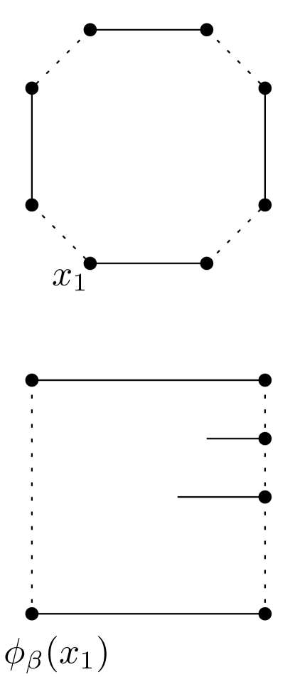
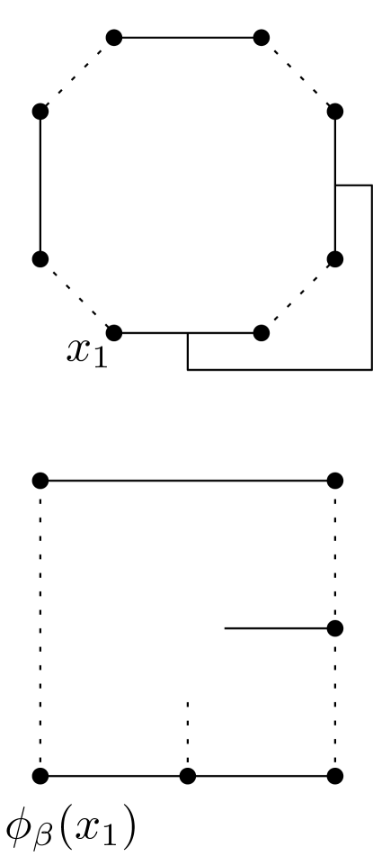
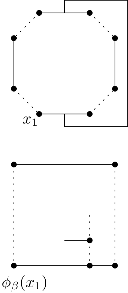
We still fix a boundary condition with link endpoints ordered as in (1.1) and such that . In Lemma 3.3, we have constructed a discrete holomorphic observable . In the course of the present and the subsequent sections, we will see that it converges as to its continuum analogue: a conformal map from the polygon onto a certain slit rectangle depending on , explicitly given in terms of a (degenerate) Schwarz-Christoffel mapping, and uniquely determined by the boundary data in Lemma 3.3 — for concrete examples, see Proposition 3.4 and Equation (C.1) in Appendix C, as well as Figure 3.4.
To address the convergence of the observable, we use a notion of convergence of polygons in terms of uniformizing maps with respect to the unit disc . As before, we regard any planar graph also as a planar domain by considering the union of all its vertices, edges, and faces. We say that a sequence of discrete polygons on converges as to a polygon in the Carathéodory sense202020Equivalently, this could be phrased in terms of uniformizing maps with respect to the upper half-plane . if there exist conformal maps from onto , and a conformal map from onto , such that locally uniformly on , and for all .
The convergence of the observable will hold locally uniformly in the following sense. If are functions on vertices of , we extend them to functions on the corresponding planar domains by linear interpolation. Then, we say that the sequence converges to a holomorphic function locally uniformly as if the corresponding maps converge to locally uniformly on .
Proposition 3.4.
We emphasize that the convergence of the observable does not require any additional regularity of : we only need that is locally connected. Moreover, we only require the convergence of polygons in the Carathéodory sense, that is weaker than that in Equation (1.10). These two points are essential for the proof of Theorem 1.3, since upon exploring discrete interfaces, we cannot guarantee much regularity for the boundaries of the domains thus obtained.
Proof of Proposition 3.4.
Step 1.
We use standard discrete complex analysis arguments (see, e.g. [DC13, Section 8]). If the sequence is uniformly bounded, then it has a locally uniformly convergent subsequence. The discrete holomorphicity from Lemma 3.3 implies that any discrete contour integral of any in vanishes, and this property is inherited by any contour integral of any subsequential limit, which thus is holomorphic in by Morera’s theorem.
To complete Step 1, it remains to show the uniform boundedness of , which by Lemma 3.3 is equivalent to the uniform boundedness of , for all . The latter fact can be argued via contradiction: if along some sequence , then, as above, converges locally uniformly to some holomorphic function . Now, on the one hand the limit function satisfies on , so has to be a constant, while on the other hand, from Lemma 3.3 and the discrete Beurling estimate we see that cannot be a constant. This is the sought contradiction.
Step 2.
Step 3.
Without loss of generality, we assume that and , and identify the c.c.’s and with connected components of , that is, the lower half-plane with the branch cuts introduced in Section 2.1. Consider the differential of , where are two subsequential limits. Note that
with some constants and . The Schwarz reflection principle (see, e.g., [Ahl78, Chapter 4, Section 6.5]) shows that extends to a holomorphic function
In particular, extends to a holomorphic differential on the Riemann surface associated to the hyperelliptic curve (2.8), defined as on and as on . Expanding it in the basis (2.10) of holomorphic differentials on ,
| (3.2) |
and integrating both sides of (3.2) along respectively, we see that . Since is invertible by Lemma 2.1, we obtain , so is the constant function. Because on and on , we see that equals zero. ∎
The holomorphic function is, in fact, a conformal map from the polygon to a certain slit rectangle depending on . In particular, for , the map has an explicit (degenerate) Schwarz-Christoffel formula, see Equation (C.1). Geometrically, if , then is the unique conformal map from onto a rectangle of unit width with horizontal and vertical slits such that maps the four points to the four corners of the rectangle so that , and maps c.c.’s of to vertical slits and c.c.’s of to horizontal slits, according to the boundary data (3.1). See Figure 1.2 and 3.4 for some illustrations.
3.3 Expansion near a marked point
To derive the scaling limit of the Peano curve (Theorem 1.3 in Section 3.4), we need to analyze the asymptotics of the function as approaches one of the marked points (Lemma 3.5). In particular, we will explicitly relate it to the partition function (Lemma 3.6). For definiteness and without loss of generality (by the full Möbius covariance from Proposition 2.6 and duality for the UST model), we consider the case where and we study the limit of as .
Lemma 3.5.
Both determinants can be evaluated in terms of the Vandermonde determinant: is given by the line integral analogue of (2.21) (cf. Lemma A.1 in Appendix A), and
| (3.6) | ||||
where we write , and is defined in (2.5).
Proof.
Expanding in the basis (2.10) of holomorphic differentials on and integrating, we see that the holomorphic function has the form
| (3.7) |
uniquely212121Note that is a polynomial of degree at most (in fact, exactly by (C.1) in Proposition C.1). determined by the boundary data (3.1):
| (3.8) | ||||
| (3.9) |
Indeed, as the matrix is invertible by Lemma 2.1, these equations have a unique solution , which determine the coefficients of : by (3.8, 3.9), we have
By Cramer’s rule, we have , where is the adjugate matrix of . Hence, we obtain from Cramer’s rule the relation
where are the coefficients of . Now, we obtain the desired expansion (3.3) by a direct computation. First, from (3.6, 3.7) we have
| (3.10) |
writing . Next, making the change of variables , we obtain
Now, we have
Collecting the terms according to different powers of , we obtain (3.3). ∎
3.4 Scaling limits of Peano curves — proof of Theorem 1.3
We will next complete the proof of Theorem 1.3 by deriving the limit of the law of the Peano curve in the case where (recall that the other cases can be treated via duality and rotation symmetry).
Loewner chains
Let us first collect some preliminaries on Loewner chains — see [Law05] for background. Suppose that a continuous function , called the driving function, is given. Consider solutions to the Loewner equation
| (3.12) |
For each , the ordinary differential equation (3.12) has a unique solution up to
the swallowing time of . As a function of , each map is a well-defined conformal transformation from onto , where the hull of swallowed points is . The collection of hulls growing in time is called a Loewner chain. In fact, is the unique conformal map such that as . The half-plane capacity of the hull is defined as the coefficient of in the series expansion of at infinity, and (3.12) implies that . We say that the process is parameterized by the half-plane capacity.
SLE processes
Chordal Schramm-Loewner evolution, , is the random Loewner chain driven by , a standard one-dimensional Brownian motion of speed . See [Law05, RS05] for background and further properties of this process. In this article, we assume that .
Recall that a partition function (with ) refers to a positive smooth function satisfying the PDE system (PDE) and Möbius covariance (COV). We can use any partition function to define a Loewner chain associated to : in the upper half-plane , started from , and with marked points , that is, the Loewner chain driven by the solution to the SDEs (1.8). This process is well-defined up to the first time when either or is swallowed, and each is the time-evolution of for times smaller than the swallowing time of .
Now are ready to complete the proof of Theorem 1.3. The key is to identify the driving process of the scaling limit curve as the solution to the SDEs (1.8) with and .
Proof of Theorem 1.3.
By assumption, the medial polygons converge to the polygon in the sense of Equation (1.10), so they also converge in the Carathéodory sense: there exist conformal maps and such that and, as , the maps converge to locally uniformly on , and for all .
As before, consider the UST on the primal polygon with boundary condition such that , and let be the Peano curve started from . Denote by its conformal image parameterized by half-plane capacity. By Lemma 3.1, we may choose a subsequence such that converges weakly in the space (1.9) as . We denote the limit by , define and parameterize it also by half-plane capacity. By Lemma 3.1 and a similar argument as in [HLW24, Corollary 4.11], the family is precompact in the uniform topology of curves parameterized by half-plane capacity. Thus, using the diagonal method and the Skorohod representation theorem, we may choose a subsequence, still denoted by , such that converges to locally uniformly as , almost surely.
Next, we define to be the first time when hits and the first time when hits . By properly adjusting the coupling (as in [HLW24, Proof of Theorem 4.2, Equation (4.14)]; see also [Kar20, GW20]), we may assume that almost surely.
Now, denote by the driving function of and by the corresponding conformal maps. Write for . Via a standard argument (see, e.g., [HLW24, Lemma 4.8 and Lemma 4.9]), we derive from the holomorphic observable of Proposition 3.4 the local martingale
| (3.13) |
It remains to argue that is a semimartingale and find the SDE for it. This step is also standard, see, e.g., [HLW24, Proof of Lemma 4.12] (a similar argument also appeared in [Kar20, Lemma 5.3]). For any , the function is holomorphic and not identically zero, so its zeros are isolated. Pick with large enough such that . By the implicit function theorem, is locally a smooth function of . Thus, by continuity, each time has a neighborhood for which we can choose a deterministic such that is locally a smooth function of for . This implies that is a semimartingale. To find the SDE for it, let denote the drift term of . By a computation using Itô’s formula, we find from (3.13) and using the Loewner equation (3.12) the identities
Combining this with the explicit relation (3.3) from Lemma 3.5, we find the expansion
As the drift term of has to vanish, we conclude that
| (3.14) | ||||
Recall now that the goal is to derive for the driving process the SDE
| (3.15) |
Indeed, by comparing (3.14) and (3.15) with Lemma 3.6, we see that the driving function of the curve satisfies (3.15) up to the stopping time . This completes the proof. ∎
3.5 Consequences
We conclude with another proof for the PDE system (COV) using the convergence result from Theorem 1.3 (see Corollary 3.7), and then comment briefly on the relation of our work to that of Dubédat [Dub07, Dub06].
Corollary 3.7.
For each , the function satisfies the PDE system (PDE).
Note that we already know that the function is smooth, by its explicit formula (1.2).
Proof.
The PDEs follow from the commutation relations for SLEs [Dub07]. Take any disjoint localization neighborhoods of the marked points (cf. [KP16, Appendix A]), and approximate them by on the medial lattice. For each , let be the Peano curve started from and stopped when it exits . Thanks to the precompactness (Lemma 3.1), we find a sequence such that the collection converges weakly to some collection of curves on , with law . It follows that this family of probability measures has the following properties.
-
•
Conformal invariance. For any conformal map , the law of the curve collection is the same as .
-
•
Domain Markov property. Given initial segments up to some stopping times , the remaining parts have the law , where
-
•
For each , the marginal law of is the same as the law of the Loewner chain with driving function (1.11) started from and stopped when it exits .
It thus follows from [Dub07, Theorem 7] that satisfies the asserted PDEs (PDE). ∎
Remark 3.8.
4 Crossing probabilities, groves, and pure partition functions
In this section, we prove the explicit formulas for the scaling limits of crossing probabilities of the UST Peano curves (Theorem 1.4 in Section 4.1). In the cases and , the crossing probability formulas are evident, as they are just given by the meander entries already in the discrete model. Explicitly, we have
The probabilities in Theorem 1.4 become interesting when , still retaining some combinatorial structure. Indeed, Kenyon and Wilson [KW11] provided a systematic method for calculating the discrete crossing probabilities for groves, including spanning trees.
Groves
Consider the discrete polygon whose each boundary arc with is wired and these wired arcs are isolated outside of . Following [KW11], we define a grove to be a spanning forest of such that each of its component trees contains at least one wired arc. Note that every grove induces a non-crossing partition on the wired arcs, which we view as a non-crossing partition of . Every grove also induces non-intersecting Peano curves connecting the points pairwise. The endpoints of these Peano curves form a planar link pattern , and these two are in bijection (via the correspondence illustrated in Figure 3.2): we write .
Crossing probabilities of the UST Peano curves can be expressed in terms of more general crossing probabilities for groves. We consider a random grove sampled from the uniform distribution of all groves on and denote the random induced non-crossing partition by . Then, [KW11, Theorem 1.2] gives the following probabilities:
| (4.1) |
where the sum is taken over all (possibly crossing) partitions of , the factor is a constant which only depends on and , and the combinatorial factor is
where the sum is taken over all those spanning forests of the -complete graph whose trees induce the partition , the product over edges in the forest , and the summands are currents between the vertices and , that is, negatives of the entries of the Dirichlet-to-Neumann matrix of the -complete graph (see [KW11, Appendix A]). Concretely, can be written in terms of differences of boundary values of discrete holomorphic functions as follows. For each , let be the discrete holomorphic function with boundary data222222Throughout, we use the cyclic indexing convention etc. (it is not hard to see that is uniquely determined)
| (4.2) |
Write for the constant values on the arcs , so . Then,
Similarly as in the proof of Proposition 3.4, we see that if the primal polygons converge to a polygon in the Carathéodory sense as , then converges locally uniformly as to the unique holomorphic function on with boundary data analogous to (4.2). Note that is the unique conformal map from onto the rectangle of unit width with horizontal slits such that maps to the four corners of the rectangle with , and it maps each to horizontal slits, for .
From these observables we readily obtain the convergence of the crossing probabilities of the UST Peano curves (Proposition 4.1 in Section 4.1). In Section 4.2, we derive the asymptotic properties (-ASY1,1, -ASY1,3) of the pure partition functions , thereby verifying a part (ASY) of Theorem 1.2. We complete the proof of Theorems 1.1 and 1.2 in Section 4.3.
4.1 Crossing probabilities — proof of Theorem 1.4
Let us now consider the UST Peano curves. For each , the endpoints of these curves give rise to a random planar link pattern in . From Equation (4.1), we obtain a formula for the crossing probabilities:
and where the sum is taken over all partitions of and the sum is taken over all planar link patterns . The results of [KW11] imply that is a matrix whose elements equal or , and each row of contains at least one non-zero element (see more details in [KW11, Section 2.3]). In particular, we readily obtain that the UST crossing probabilities in Theorem 1.4 have conformally invariant scaling limits. We emphasize that, for this we only require the convergence of polygons in the Carathéodory sense, that is weaker than (1.10). Also, we do not require any additional regularity of here — we only need that is locally connected.
Proposition 4.1.
Fix and a polygon . Suppose that a sequence of primal polygons converges to in the Carathéodory sense as . For any with , the following limit exists and is positive:
| (4.3) |
Furthermore, the limit satisfies the following properties.
-
1.
Conformal invariance: For any conformal map on , we have
(4.4) -
2.
Smoothness: is a smooth function on .
Proof.
See 1.4
4.2 Asymptotics of pure partition functions
The purpose of this section is to verify the asymptotic properties (ASY) (-ASY1,1, -ASY1,3) of the pure partition functions in Theorem 1.2.
Throughout, fix and . We will use the following two operations on planar link patterns.
-
•
Link removal: , a map , where is the link pattern obtained from by removing and relabeling the remaining indices by . Note that is a bijection.
-
•
Link tying: , a map , where is the “tying operation” defined by
(4.6) where (resp. ) is the pair of (resp. ) in (and are unordered) — see Figure 4.1. Note that is a surjection, but not a bijection.
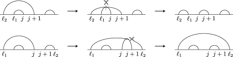
Lemma 4.2.
Fix . The following properties hold for the symmetric matrix (1.6).
-
1.
If and , then we have and .
-
2.
If and , then we have .
-
3.
If , then there exists such that and .
Proof.
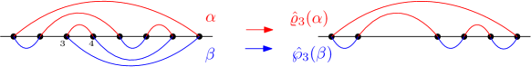
To prove the asymptotic properties (-ASY1,1 -ASY1,3) of the pure partition functions defined in Equation (1.7), we make use of the corresponding properties (-ASY1,1 -ASY1,3) of the Coulomb gas functions
| (4.7) |
Lemma 4.3.
Let . Fix and suppose . Then, for all , the following asymptotic property holds:
| (4.8) |
where and .
Proof.
Lemma 4.4.
Proof.
Pick satisfying . By (4.7), we have
Taking the limit of both sides232323Note that we already know that the limits exist by Proposition 2.9 and Equation (1.7)., we see by (-ASY1,3) (from Proposition 2.9) that
also noting that the terms with vanish in this limit by the property (4.8) from Lemma 4.3 for . Invoking again the relation (4.7) (applied to ), we obtain
also using using Item 2 of Lemma 4.2 to write . After re-indexing the sum via the bijection , recalling that is a surjection, and that the meander matrix is invertible, we obtain (4.9). ∎
Lemma 4.5.
Proof.
Pick satisfying . By (4.7) and Item 1 of Lemma 4.2, we have
Taking the limit of both sides242424Note that from Theorem 1.4, we know that the summands are positive., we see by (-ASY1,1) (from Proposition 2.9) that
Invoking again the relation (4.7) (applied to ), we obtain
Using the bijection and the inverse meander matrix, we obtain (4.10):
This shows the asserted asymptotics property (4.10). ∎
4.3 Finishing the proofs of Theorems 1.1 and 1.2
- •
- •
- •
- •
- •
-
•
We have due to Proposition 2.14.
-
•
The positivity of follows because and when .
It remains to show the linear independence of both collections and . We give an argument based on the asymptotic properties (-ASY1,1) and (-ASY1,3) of . For with for (but not with link endpoints ordered as in (1.1)), we say that the ordering of links is allowable if all links of can be removed in the order in such a way that at each step, the link to be removed connects two consecutive indices (cf. [FK15, PW19]). Note that each has at least one allowable ordering. For such a choice, the iterated limit
at , with , is well-defined for any function in the span of or . Thus, it defines a linear operator on either span. Furthermore, (-ASY1,1, -ASY1,3) yield
This implies that the collection is linearly independent. As the meander matrix (1.6) is invertible, by definition (1.7) of , it gives rise to a change of basis between and , so the latter collection is linearly independent too. ∎
Appendix A Period matrices for cycles and intervals
We record here a useful identity relating the two matrices (2.12, 2.13). As a warm-up, note that by deforming and decomposing the integration of along the loop into the integration along the interval and times the same negatively oriented interval, we have
| (A.1) |
In general, we have the following upper-triangular transformation.
Lemma A.1.
We have , where is an upper-triangular matrix with entries
| (A.2) |
Proof.
From the decompositions of the integrals of along on the one hand, and along on the other hand, into linear combinations
| (A.3) | ||||
| (A.4) |
it is clear that for all and for all such that . To find the non-zero entries with , note that by (A.3, A.4),
| [as in (A.2)] | ||||
where we used the fact that the parity of and is always different. This shows that have the claimed form (A.2). The general formula follows inductively. ∎
Appendix B Examples of partition functions
As examples, let us discuss for the special cases of and .
Lemma B.1.
Take in (2.19). For and , we have
Proof.
By the branch choice for , setting , we have
where denotes the principal branch of the square root. ∎
Lemma B.2.
Note also that is the elliptic integral of the first kind, which is not a surprise given the relation (2.23) of and to the -cycles in Section 2.3.
Proof.
We first show (B.1). Proposition 2.4 gives
where is the loop surrounding and . Using (A.1) and the branch choice of , we obtain
where is defined in (2.4). To simplify this, writing and setting , we have , and using also [AS92, Eq. (17.2.6), Eq. (17.3.9)], we obtain
which gives (B.1). The identity (B.2) then follows from (B.1) and Propositions 2.6 and 2.14. ∎
Appendix C Schwarz-Christoffel type conformal mappings
The goal of this appendix is to derive another explicit expression for the observable on , compared to the one (3.10) found in the proof of Lemma 3.5. For definiteness and without loss of generality (by the full Möbius covariance from Proposition 2.6 and duality for the UST model), we consider the case where .
Proposition C.1.
On , the holomorphic function with boundary data (3.1) (cf. Proposition 3.4) has the explicit formula252525Note that (C.1) is the same for any branch choice, since the multiplicative phase factors from the numerator and denominator cancel out.
| (C.1) |
where is the meromorphic function (2.9) on , and
is a monic polynomial with roots and coefficients determined as the unique solution to the linear system
| (C.2) |
is a line integral counterpart of a matrix involving -periods of holomorphic one-forms (2.10). Here, is the submatrix of obtained by removing the last row.
Note that is a Schwarz-Christoffel map [Ahl78, Chapter 6, Section 2.2], conformal from onto a slit rectangle. The accessory parameters are those points on the real line which are mapped to the tips of the slits in the image of . See Figure 1.2 for an illustration.
Proof.
Let be the principal submatrix of obtained by removing the last row and the last column. Expanding according to the cofactors along the last row, we have
where is the minor obtained from by removing the last row and :th column. Thus, we see that
which implies by Lemma 2.1 that is invertible and the linear system (C.2) has a unique solution. It remains to note by (C.2) that the function (C.1) satisfies the boundary data (3.1) from Proposition 3.4, which determines uniquely. ∎
Appendix D Identifying Peano curves with given connectivity
The main purpose of this appendix is to verify the following property, needed in the proof of Theorem 1.4 in Section 4.1. We shall use the notations from Section 4.
Proposition D.1.
For all such that , we have
This quantity also describes the conditional laws of the scaling limit curves for each connectivity (in the spirit of Doob’s transform), as stated in the following result. As in the proof of Theorem 1.3, we will fix a sequence of conformal maps and such that and, as , the maps converge to locally uniformly on , and for all . We consider the Peano curve started from in the scaling limit.
Proposition D.2.
In particular, combining Propositions D.1 & D.2, we see that the marginal law in the latter is given by the Loewner chain associated to the pure partition function .
D.1 Marginal law — proof of Proposition D.2
When , we denote by
the conditional law of given the event that the planar link pattern induced by the Peano curves equals .
Lemma D.3.
The following properties hold for the conditional law .
-
1.
The family of laws is precompact in the curve space (1.9).
-
2.
The law does not depend on the choice of the b.c. .
Proof.
Property 1 is a consequence of Lemma 3.1 and (4.3). For Property 2, recall that each grove induces Peano curves whose endpoints form a planar link pattern, and note that the conditional law of the grove Peano curve started from given the event is the same as . The former is independent of , as claimed. ∎
Next, we focus on the Peano curve started from and study its scaling limit (). In the continuum, we can relate the setup on to the setup on via conformal invariance. In , we denote . From Theorem 1.3, we already know that the scaling limit of the Peano curve is given by , where is the Loewner chain associated to the partition function started from , i.e., the driving function of is the solution to the following system of SDEs:
| (D.1) |
Let be the first time when is swallowed.
Lemma D.4.
Assume the same setup as in Theorems 1.3 and 1.4. Fix such that . The following process is a positive martingale with respect to the filtration generated by :
| (D.2) |
Moreover, the law converges weakly to the law of weighted by . In particular, it converges weakly to the Loewner chain associated to started from up to time .
The proof follows a routine argument, which we outline below.
Proof.
Let be the first time when hits . For every , define to be the component of with and on its boundary. Define also to be the primal graph associated to and define to be the primal vertex of nearest to . Thanks to the domain Markov property of our model, the conditional crossing probability associated to the interface gives a tautological martingale (with respect to the filtration generated by ):
where we denote262626We also denote by the corresponding expectation. by the law of the UST on the primal polygon with b.c. . We define the stopping times
and we similarly define the stopping times for . We may assume that almost surely, by considering continuous modifications (see more details in [Kar19, Appendix B]). Now, we find
| (D.3) |
for any bounded continuous function . Let us consider the two sides of (D.3) separately.
- •
- •
In conclusion, for any , we have
Indeed, a similar argument272727Here, it is important that the limit of does not hit any points in except at its endpoint (Lemma 3.1). as in [HLW24, Proof of Theorem 4.2] shows that converge almost surely to a time at least . By the Radon-Nikodym theorem, this implies that up to time , the process defined in (D.2) is a martingale for , and the limit of is the same as weighted by . Furthermore, as the driving function of satisfies (D.1), Girsanov’s theorem yields
where is a Brownian motion under the law of . Combining this with (D.1), we see that has the same law as the Loewner chain associated to . ∎
D.2 Asymptotics of crossing probabilities
In the proof of Proposition D.1, we will need the following asymptotics property of the limit crossing probabilities.
Lemma D.5.
Fix and a polygon whose boundary is a -Jordan curve. Fix and suppose and . Then, the function defined in Proposition 4.1 has the following asymptotics: for all and , we have
| (D.4) |
where and .
Proof.
To facilitate notation, we take without loss of generality. So we assume and write . To prove (D.4), we approximate by discrete polygons in the same setup as in Theorem 1.3, i.e., in the sense of (1.10). Note that at this point, the results of Theorem 1.3 and Proposition 4.1 are already at our disposal. In particular, (4.3) immediately gives
To prove (D.4), we shall consider the double-limit of as and .
Let denote the Peano curve starting from . Pick much larger than the diameter of the arc but much smaller than the distance between and . With fixed, write
| (D.5) |
We consider the two terms on the right-hand side separately.
-
•
First term on RHS of (D.5): A sample of the UST can be generated using loop-erased random walks (LERW) via Wilson’s algorithm [Wil96] (see also [Sch00, Section 2]). Note that, on the event , if , then the LERW branch in the dual tree connecting the arcs and goes outside of . Thus, it follows from the Beurling estimate for simple random walk (see, e.g., [Sch00, Lemma 2.1]) that
where are universal constants and the right-hand side is uniform in .
-
•
Second term on RHS of (D.5): By our choice of , we have
By precompactness (Lemma 3.1), has a subsequential weak scaling limit , and we may couple the convergent subsequence so that it converges almost surely. Note that the connected component of with on its boundary converges in the Carathéodory sense to the connected component of with on its boundary (by a standard argument, see, e.g. [GW20]). Therefore, Proposition 4.1 shows that, almost surely,
where is the conformal map from the connected component of with on its boundary onto fixing and , and we write . In conclusion, as we obtain the following bounds for the second term on the RHS of (D.5):
Collecting these estimates and taking “”, resp. “”, we obtain
To finish, after taking first the limit (note that is a smooth function of the marked points by Item 2 of Proposition 4.1) and then the limit , we obtain
which gives (D.4) and concludes the proof. ∎
Lemma D.6.
Fix and and suppose and . Then, for all , we have
| (D.6) |
where and .
D.3 Proof of Proposition D.1
Proof of Proposition D.1.
We denote the quantity of interest as
On the one hand, by Lemma D.3 the limit of is independent of , while on the other hand, by Lemma D.4 it is the same as the law of the Loewner chain associated to . This implies that is independent of (note that is a smooth function of the marked points by Item 2 of Proposition 4.1). Moreover, by rotation symmetry of the UST model, we see that is independent of for all . Thus, for any , the quantity is independent of . This shows that the following ratio is a constant:
It suffices to show that . We prove this by induction on . The case of being trivial, we assume that , and pick such that . Then, for all , from the asymptotics (D.6) in Lemma D.6 and the induction hypothesis, we find that
This shows that the quantity is independent of as long as . It remains to identify it with the pure partition function defined in (1.7). By Proposition 4.1, as a sum of total probability, we have , so
Inverting the matrix and recalling the definition (1.7), we obtain . ∎
References
- [Ahl78] Lars V. Ahlfors. Complex analysis. McGraw-Hill Book Co., New York, third edition, 1978.
- [AS92] Milton Abramowitz and Irene A. Stegun. Handbook of mathematical functions with formulas, graphs, and mathematical tables. Dover Publications, Inc., New York, 1992. Reprint of the 1972 edition.
- [BB03] Michel Bauer and Denis Bernard. Conformal field theories of stochastic Loewner evolutions. Comm. Math. Phys., 239(3):493–521, 2003.
- [BBK05] Michel Bauer, Denis Bernard, and Kalle Kytölä. Multiple Schramm-Loewner evolutions and statistical mechanics martingales. J. Stat. Phys., 120(5-6):1125–1163, 2005.
- [BPZ84] Alexander A. Belavin, Alexander M. Polyakov, and Alexander B. Zamolodchikov. Infinite conformal symmetry in two-dimensional quantum field theory. Nucl. Phys. B, 241(2):333–380, 1984.
- [BLR20] Nathanaël Berestycki, Benoît Laslier, and Gourab Ray. Dimers and imaginary geometry. Ann. Probab., 48(1):1–52, 2020.
- [Car84] John L. Cardy. Conformal invariance and surface critical behavior. Nucl. Phys. B, 240(4):514–532, 1984
- [Car99] John L. Cardy, Logarithmic correlations in quenched random magnets and polymers. Preprint in arXiv:cond-mat/9911024, 1999.
- [Car03] John L. Cardy. Stochastic Loewner evolution and Dyson’s circular ensembles. J. Phys. A, 36(24):L379–L386, 2003.
- [CHI21] Dmitry Chelkak, Clément Hongler, and Konstantin Izyurov. Correlations of primary fields in the critical planar Ising model. Preprint in arXiv:2103.10263, 2021.
- [CR13] Thomas Creutzig and David Ridout. Logarithmic conformal field theory: Beyond an introduction. J. Phys. A, 46(49):494006, 2013.
- [DC13] Hugo Duminil-Copin. Parafermionic observables and their applications to planar statistical physics models. Volume 25 of Ensaios Matemáticos. Sociedade Brasileira de Matemática, Rio de Janeiro, 2013.
- [DF84] Vladimir S. Dotsenko and Vladimir A. Fateev. Conformal algebra and multipoint correlation functions in 2D statistical models. Nucl. Phys. B, 240(3):312–348, 1984.
- [DFGG97] Philippe Di Francesco, Olivier Golinelli, and Emmanuel Guitter. Meanders and the Temperley-Lieb algebra. Comm. Math. Phys., 186(1):1–59, 1997.
- [DFMS97] Philippe Di Francesco, Pierre Mathieu, and David Sénéchal. Conformal field theory. Graduate Texts in Contemporary Physics. Springer-Verlag, New York, 1997.
- [Dub06] Julien Dubédat. Euler integrals for commuting SLEs. J. Stat. Phys., 123(6):1183–1218, 2006.
- [Dub07] Julien Dubédat. Commutation relations for Schramm-Loewner evolutions. Comm. Pure Appl. Math., 60(12):1792–1847, 2007.
- [Dub09] Julien Dubédat. SLE and the free field: partition functions and couplings. J. Amer. Math. Soc., 22(4):995–1054, 2009.
- [Dub15] Julien Dubédat. and Virasoro representations: localization. Comm. Math. Phys., 336(2):695–760, 2015.
- [Dup04] Bertrand Duplantier. Conformal fractal geometry and boundary quantum gravity. In Fractal Geometry and Applications: A Jubilee of Benoît Mandelbrot, Vol. 72 of Proceedings of Symposia in Pure Mathematics, p. 365-482. American Mathematical Society, Providence, R.I., 2004.
- [FK92] Hershel M. Farkas and Irwin Kra. Riemann surfaces. Vol. 71 of Graduate Texts in Mathematics. Springer-Verlag, New York, second edition, 1992.
- [FF84] Boris L. Feĭgin and Dmitry B. Fuchs. Verma modules over the Virasoro algebra. In Topology (Leningrad 1982). Vol. 1060 of Lecture Notes in Mathematics, pp. 230–245. Springer-Verlag, Berlin Heidelberg, 1984.
- [FPW24] Yu Feng, Eveliina Peltola, and Hao Wu. Connection probabilities of multiple FK-Ising interfaces. Probab. Theory Related Fields, 189(1-2):281–367, 2024.
- [FK15] Steven M. Flores and Peter Kleban. A solution space for a system of null-state partial differential equations: Parts 1-4. Comm. Math. Phys., 333(1-2):389–715, 2015.
- [FSKZ17] Steven M. Flores, Jacob J. H. Simmons, Peter Kleban, and Robert M. Ziff. A formula for crossing probabilities of critical systems inside polygons. J. Phys. A, 50(6):064005, 2017.
- [GK96] Matthias R. Gaberdiel and Horst G. Kausch. Indecomposable fusion products. Nucl. Phys. B, 477(1):293–318, 1996.
- [GW20] Christophe Garban and Hao Wu. On the convergence of FK-Ising percolation to SLE. J. Theor. Probab., 33(2):828–865, 2020.
- [Gur93] Victor Gurarie. Logarithmic operators in conformal field theory. Nucl. Phys. B, 410(3):535–549, 1993.
- [HLW24] Yong Han, Mingchang Liu, and Hao Wu. Hypergeometric SLE with : Convergence of UST and LERW in topological rectangles. Ann. Inst. H. Poincaré Probab. Statist. to appear, 2024. Preprint in arXiv:2008.00403.
- [Izy15] Konstantin Izyurov. Smirnov’s observable for free boundary conditions, interfaces and crossing probabilities. Comm. Math. Phys., 337(1):225–252, 2015.
- [Izy22] Konstantin Izyurov. On multiple SLE for the FK-Ising model. Ann. Probab., 50(2):771–790, 2022.
- [Kar19] Alex Karrila. Multiple SLE type scaling limits: from local to global. Preprint in arXiv:1903.10354, 2019.
- [Kar20] Alex Karrila. UST branches, martingales, and multiple . Electron. J. Probab., 25(83):1–37, 2020.
- [KKP20] Alex Karrila, Kalle Kytölä, and Eveliina Peltola. Boundary correlations in planar LERW and UST. Comm. Math. Phys., 376(3):2065–2145, 2020.
- [Kau00] Horst G. Kausch. Symplectic fermions. Nucl. Phys. B, 583(3):513–541, 2000.
- [Ken01] Richard Kenyon. Dominos and the Gaussian free field. Ann. Probab., 29(3):1128–1137, 2001.
- [KL07] Michael J. Kozdron and Gregory F. Lawler. The configurational measure on mutually avoiding paths. Fields Inst. Commun., 50:199–224, 2007.
- [KRV20] Antti Kupiainen, Rémi Rhodes, and Vincent Vargas. Integrability of Liouville theory: proof of the DOZZ Formula. Ann. of Math. (2), 191(1):81–166, 2020.
- [GKR23] Colin Guillarmou, Antti Kupiainen, and Rémi Rhodes. Compactified imaginary Liouville theory. Preprint in arXiv:2310.18226, 2023.
- [KP16] Kalle Kytölä and Eveliina Peltola. Pure partition functions of multiple SLEs. Comm. Math. Phys., 346(1):237–292, 2016.
- [KP20] Kalle Kytölä and Eveliina Peltola. Conformally covariant boundary correlation functions with a quantum group. J. Eur. Math. Soc., 22(1):55–118, 2020.
- [KW11] Richard W. Kenyon and David B. Wilson. Boundary partitions in trees and dimers. Trans. Amer. Math. Soc., 363(3):1325–1364, 2011.
- [Kyt09] Kalle Kytölä. SLE local martingales in logarithmic representations. J. Stat. Mech., 0908:P08005, 2009.
- [KR09] Kalle Kytölä and David Ridout. On staggered indecomposable Virasoro modules. J. Math. Phys., 50:123503, 2009.
- [Law05] Gregory F. Lawler. Conformally invariant processes in the plane. Volume 114 of Mathematical Surveys and Monographs. American Mathematical Society, Providence, RI, 2005.
- [Law09] Gregory F. Lawler. Partition functions, loop measure, and versions of SLE. J. Stat. Phys., 134(5-6):813–837, 2009.
- [LSW01] Gregory F. Lawler, Oded Schramm, and Wendelin Werner. Values of Brownian intersection exponents I: Half-plane exponents. Acta Math., 187(2):237–273, 2001.
- [LSW04] Gregory F. Lawler, Oded Schramm, and Wendelin Werner. Conformal invariance of planar loop-erased random walks and uniform spanning trees. Ann. Probab., 32(1B):939–995, 2004.
- [LW23] Mingchang Liu and Hao Wu. Loop-erased random walk branch of uniform spanning tree in topological polygons. Bernoulli, 29(2):1555–1577, 2023.
- [MR07] Pierre Mathieu and David Ridout. From percolation to logarithmic conformal field theory. Phys. Lett. B, 657:120–129, 2007.
- [MS17] Jason Miller and Scott Sheffield. Imaginary geometry IV: interior rays, whole-plane reversibility, and space-filling trees. Probab. Theory Related Fields, 169(3-4):729–869, 2017.
- [Nie87] Bernard Nienhuis. Coulomb gas formulation of two-dimensional phase transitions. In Phase Transitions and Critical Phenomena, Vol. 11, pp. 1-53. Academic Press, London, 1987.
- [PR07] Paul A. Pearce and Jørgen Rasmussen. Solvable critical dense polymers. J. Stat. Mech., 0702:P02015, 2007.
- [Pel19] Eveliina Peltola. Towards a conformal field theory for Schramm-Loewner evolutions. J. Math. Phys., 60(10):103305, 2019.
- [PW19] Eveliina Peltola and Hao Wu. Global and local multiple SLEs for and connection probabilities for level lines of GFF. Comm. Math. Phys., 366(2):469-536, 2019.
- [PW23] Eveliina Peltola and Hao Wu. Crossing probabilities of multiple Ising interfaces. Ann. Appl. Probab., 33(4):3169–3206, 2023.
- [Pol70] Alexander M. Polyakov. Conformal symmetry of critical fluctuations. JETP Lett., 12(12):381–383, 1970.
- [RS07] Nicholas Read and Hubert Saleur. Associative-algebraic approach to logarithmic conformal field theories. Nucl. Phys. B, 777(3):316–351, 2007.
- [RS05] Steffen Rohde and Oded Schramm. Basic properties of SLE. Ann. of Math. (2), 161(2):883–924, 2005.
- [Roh96] Falk Rohsiepe. On reducible but indecomposable representations of the Virasoro algebra. BONN-TH-96-17, 1996.
- [Rue13] Philippe Ruelle. Logarithmic conformal invariance in the Abelian sandpile model. J. Phys. A, 46(49):494014, 2013.
- [SV14] Raoul Santachiara and Jacopo Viti. Local logarithmic correlators as limits of Coulomb gas integrals. Nucl. Phys. B, 882(1):229–262, 2014.
- [Sch08] Martin Schottenloher. A mathematical introduction to conformal field theory. Vol. 759 of Lecture Notes in Physics. Springer-Verlag, Berlin Heidelberg, 2nd edition, 2008.
- [Sch00] Oded Schramm. Scaling limits of loop-erased random walks and uniform spanning trees. Israel J. Math., 118(1):221–288, 2000.
- [Sch06] Oded Schramm. Conformally invariant scaling limits: an overview and a collection of problems. In International Congress of Mathematicians. Vol. I, pp. 513–543. Eur. Math. Soc., Zürich, 2006.
- [Smi01] Stanislav Smirnov. Critical percolation in the plane: conformal invariance, Cardy’s formula, scaling limits. C. R. Acad. Sci. Paris Sér. I Math., 333(3):239–244, 2001.
- [Smi06] Stanislav Smirnov. Towards conformal invariance of 2D lattice models. In International Congress of Mathematicians. Vol. II, pp. 1421–1451. Eur. Math. Soc., Zürich, 2006.
- [Wil96] David B. Wilson. Generating random spanning trees more quickly than the cover time. In Proceedings of the Twenty-eighth Annual ACM Symposium on the Theory of Computing (Philadelphia, PA, 1996), pp. 296–303. ACM, New York, 1996.
- [Wu20] Hao Wu. Hypergeometric SLE: conformal Markov characterization and applications. Comm. Math. Phys., 374(2):433-484, 2020.
- [WZ17] Hao Wu and Dapeng Zhan. Boundary arm exponents for SLE. Electron. J. Probab., 22(89):1–26, 2017.