Uniform position alignment estimate of spherical flocking model with inter-particle bonding forces
Abstract.
We present a sufficient condition of the complete position flocking theorem for the Cucker-Smale type model on the unit sphere with an inter-particle bonding force. For this second order dynamical system derived in [Choi, S.-H., Kwon, D. and Seo, H.: Cucker-Smale type flocking models on a sphere. arXiv preprint arXiv:2010.10693, 2020] by using the rotation operator in three dimensional sphere, we obtain an exponential decay estimate for the diameter of agents’ positions as well as time-asymptotic flocking for a class of initial data. The sufficient condition for the initial data depends only on the communication rate and inter-particle bonding parameter but not the number of agents. The lack of momentum conservation and the curved space domain make it difficult to apply the standard methodology used in the original Cucker-Smale model. To overcome this and obtain a uniform position alignment estimate, we use an energy dissipation property of this system and transform the Cucker-Smale type flocking model into an inhomogeneous system of differential equations of which solution contains the position and velocity diameters. The coefficients of the transformed system are controlled by the communication rate and a uniform upper bound of velocities obtained by the energy dissipation.
1. Introduction
Many species in nature such as birds, fish, and small germs form cluster to survive. Researchers have conducted various studies to understand this clustering phenomenon for the past several decades [3, 18, 37, 38]. The flexility for real world applications is one of the major reasons why this phenomenon attracts attention from the many researchers. For example, the effective control of a large number of unmanned drones by imitating nature is one of popular topics in the engineering community [5, 7, 11]. For the development of a surveillance system, a flocking algorithm is used to cover large areas with limited resources and to track targets [33]. This flocking phenomenon also has been widely used in various fields and has been studied intensively in the last decade. In particular, the Cucker-Smale (C-S) model is one of important models that sparked various types of mathematical researches in this field.
Cucker and Smale [12] introduced a system of ordinary differential equations (ODEs) given by
where and are the position and the velocity of the th agent for , respectively. Moreover, is the communication rate between th and th agents. We notice that the C-S model contains the acceleration term described by weighted internal relaxation forces.
In this paper, we focus on the complete position alignment of the corresponding C-S type flocking model on a sphere when it contains an inter-particle bonding force. We present a new framework to obtain the complete position flocking under a sufficient condition of initial data. We emphasize that our condition for the complete position flocking is independent of the number of agents. In particular, we prove that this second order dynamical system has a uniform exponential decay rate for the diameter of agents’ positions.
From the nature of the model on sphere, the avoidance of antipodal points is necessary to guarantee the formation of a group as in Definition 1.2. However, due to the curved geometry, it is hard to control the position diameter of ensemble , even assuming sufficiently fast velocity alignment. Thus, motivated by the flat space case studied in [28], we have added a modified inter-particle bonding force to the flocking model on sphere to control the position diameter in our previous paper [9]. Due to the geometric property of sphere, a direct application of the bonding force term in to the model on a sphere may disrupt the motion on the sphere. Instead, we employ a coupling force based on the Lohe operator in [8, 23] and derive the following flocking model [9] on a sphere with inter-particle bonding forces:
| (1.1a) | ||||
| (1.1b) | ||||
where is the communication rate between th and th agents and is a rotation operator given by
and for ,
| (1.2) |
Here, , and are three dimensional column vectors. We will discuss the properties of the rotational operator in detail in the next section.
The third term in the right hand side of (1.1b) is one of the cooperative control laws and is the inter-particle bonding force rate. We note that (1.1b) only contains the attractive force. In general, the cooperative control law consists of the sum of attractive and repulsive forces. See [10]. The research on the cooperative control law of multi-agent systems such as (1.1) is steadily increasing [26, 30] in the engineering field after the development of wireless communication technology. The flocking, agreement, formation and collision avoidance are their main subjects [21, 25, 27, 33]. For example, in [13], the opinions of committee are regarded as points and the conditions for convergence are provided. The authors in [31] proposed a controller that yields the angular position synchronization of robot systems. Recently, for practical reasons, the research has been conducted in several restricted cases such as system without velocity information [1, 31], limited visibility robots [4, 16] and objects on a sphere [19, 21]. In these studies, consensus algorithms was used to allow the individuals in the system to behave as one group. The corresponding natural rendezvous concept is given by
By using the rotation operator , we can also define the flocking on a sphere.
Definition 1.2.
[9] A dynamical system on a sphere has time-asymptotic flocking if its solution satisfies the following conditions:
-
•
(velocity alignment) the relative velocity of any two agents goes to zero as time goes to :
-
•
(antipodal points avoidance) any two agents are not located at the antipodal points for all :
In [9], we obtain that the flocking model has the velocity alignment property for any . The model has the time-asymptotic flocking for a given with the initial data satisfying a sufficient condition depending on , , and . See Theorem 2.5 in Section 2. The purpose of this paper is to remove the dependence of and obtain an exponential decay rate. The following energy functional, motivated by [28], plays a crucial role in the proof of the main theorem in this paper as well as [9].
Definition 1.3.
For a solution to (1.1), the energy functional is defined by
| (1.3) |
We note that in [9], to obtain the antipodal avoidance or the velocity alignment, the main difficulty comes from the last term of the operator given in (1.2):
| (1.4) |
Due to this term, can be singular when for some . This antipodal configuration corresponds to in the original C-S case. Even assuming an exponentially fast flocking, we cannot control the position diameter due to geometric constraints. In [9], to avoid this singularity and obtain the flocking theorem for the inter-particle bonding force, we first construct energy inequality:
This energy inequality yields a uniform positive lower bound of under a sufficient condition of initial data depending on the number of agents . For more details, see [9]. From this bound, we showed uniform Lipschitzness of as well as and we concluded that the asymptotic flocking occurs by Barbalat’s lemma.
However, with reference to the flat space case, it is a natural expectation that asymptotic exponential rendezvous will happen and the sufficient condition of initial data is independent of the number of agents . To obtain the uniform position alignment for the spherical model in (1.1), we crucially use the boundedness of the energy and the modulus conservation property of . Unlike the flocking result in [9], in the complete position alignment point of view, and terms in the rotation operator causes the main difficulty, but the modulus conservation property of via (1.4) enables us to prove our main result.
Throughout this paper, we assume that the communication rate satisfies
-
,
-
is a nonnegative strictly decreasing function with ,
-
is function on .
With this assumptions on , we obtain the following complete position flocking result.
Theorem 1.
Assume that satisfies - and the initial data satisfy that
| (1.5) |
Then the solution to (1.1) has time-asymptotic flocking on a unit sphere and exponential rendezvous
where , , , , and are positive constants depending on and only.
Remark 1.1.
- (1)
-
(2)
In [10], we obtain that there is such that if
(1.6) then the ensemble has an asymptotic rendezvous. Combining this result and Theorem 1, we can remove the condition in (1.5) and obtain the exponential convergence result. The condition in (1.6) is essential since the ensemble satisfying and has not an asymptotic rendezvous.
- (3)
The rest of this paper is organized as follows. In Section 2, we review the definition of the flocking on the sphere and provide the derivation of the C-S type model with the inter-particle bonding forces and the properties of rotation operator . In Section 3, we provide a reduction from (1.1) to an inhomogeneous system of differential equations. In Section 4, we present the proof of the asymptotic convergence result in Theorem 1 for the system with the inter-particle bonding forces. In Section 5, we use numerical simulations to confirm that our analytic results are almost optimal. Finally, Section 6 is devoted to the summary of our main results.
Notation: After normalization, we consider that the domain is a unit sphere defined by
and we set
For a given , we use to denote the standard inner product in and the standard symbol
to denote the -norm.
2. Flocking model with Lagrange multiplier and inter-particle bonding forces
In this section, we review the definition of the flocking on the sphere in general geometrical setting and the results for the rotation operator and the energy functional from [9]. The properties of the rotation operator and the energy functional are essential ingredient for the proof of our main theorem.
2.1. Relative velocity on a sphere
Unlike the flat space , in a general manifold, if two agents have different positions, the corresponding velocities are belonged to different tangent spaces, respectively. Therefore, to give the meaning that velocities in different tangent spaces are aligned, it is necessary to define a kind of transformation between two different tangent spaces. Thus, we define the following velocity difference between and at in the most geometrically canonical way:
We note that defining relative velocity is a topic that has received a lot of attention in general manifold theory. In particular, it was covered in depth in general relativity [6, 24, 32, 36]. The basic idea is largely similar, it is a parallel transport along geodesics on a manifold to compare sizes in a tangent space at one position of the manifold [6, 35]. From this general observation, a parallel transport on a sphere is characterized by a rotation matrix given in (1.2).
The central idea of a relative velocity is to consider the geodesic for two given points, which is the shortest path between two points. Then, we transport a vector field in a tangent space at one point to the tangent space at another point along the geodesic. Let be a -dimensional manifold. Note that if , then under the natural identification. For , the tangent space of at is defined as the set of all tangent vectors of at . We say that a vector field along a curve is said to be parallel along if in . Here, is the covariant derivative along obtained by the normal projection of onto the tangential plane of at . Note that geodesics in are straight lines and a constant vector is parallel along a straight line. See [14, 20, 34] for the general reference. We recall the existence and uniqueness of the parallel transport along a curve from [20].
Lemma 2.1.
[20, Theorem 4.11] Given a curve and a vector , there exists a unique parallel vector field along such that .
Note that a geodesic between two points and on a sphere is a part of a great circle containing and . Also, it is uniquely determined unless . It is well-known that the parallel transport of a vector along a great circle is given by for some rotation matrix . See Chapter 4.4 in [14]. We prove the following proposition for the sake of completeness.
Proposition 2.2.
Let be a geodesic on a sphere and . If
| (2.1) |
for all , then a vector field defined by
| (2.2) |
is parallel along , where is the rotation operator given in (1.2).
Proof.
By the symmetry of a sphere and the condition in (2.1), it is enough to consider a geodesic from to for some given by
where , , , and .
We show that is parallel along for all and . By the direct computation, it holds that
| (2.3) |
From (2.1), we can use (2.3) to obtain
Thus, it follows that
As the covariant derivatives are tangential components of above equations, is zero for all and . Note that is a basis of . Therefore, can be written as a linear combination of and and we conclude that a vector field given in (2.2) is parallel along . ∎
We emphasize that the rotation operator is an isometry as well as a bijection between two tangent spaces. We also present properties of the operator for use in the next sections.
Lemma 2.3.
For such that , and given in (1.2), it holds that
| (2.4) |
Furthermore, we have
| (2.5) |
In particular, is an orthogonal matrix, that is
| (2.6) |
Proof.
For the proof of this lemma, see Lemma 2.4 in [9]. ∎
Proposition 2.4.
is a bijection and an isometry from to .
Proof.
From (2.4) and (2.5) in Lemma 2.3, it holds that for any ,
| (2.7) |
As is a unit sphere, we have
| (2.8) |
From (2.7) and (2.8), we conclude that for any vector and thus
Furthermore, as is an orthogonal matrix from Lemma 2.3, it is invertible. By (2.5) and (2.6) in Lemma 2.3, it holds that for any ,
From (2.7), for any vector and we conclude that is a bijection.
Lastly, as is an orthogonal matrix from Lemma 2.3, it is an isometry. ∎
2.2. Lagrange multiplier and energy dissipation on a sphere
The C-S type flocking model on a sphere in (1.1) has the following property of the velocity alignment:
Here, term in the above flocking limit naturally appear from the geometric structure of the sphere. See [9] for the detailed argument. Notice that if we assume that there is a constant such that for any and , then the above limit is equivalent to
as the form of the velocity alignment in the flat space.
If the bonding force rate is large enough comparing the differences of agents’ velocities and positions, then the following flocking result with position alignment holds.
Theorem 2.5.
We revisit the idea for deriving the flocking model introduced in [9]. Then, the centripetal force term of the flocking model will be explained using the Lagrange Multiplier, and the inter-particle bonding force term corresponding to the sphere will be defined. For the consistency of initial data on the unit sphere, we consider following initial conditions:
| (2.9) |
The augmented C-S model in the Euclidean space (See [28]), the following term is added as inter-particle bonding forces:
Here, is the rate of the inter-particle bonding force. However, this term will prevent that the agent is located in the sphere. Thus, we adapt a modified inter-particle bonding force in [9]. We notice that the modified inter-particle bonding forces will be the form of Lohe operator in [23]. In summary, we consider the following model with the Lagrange multiplier for the controllability of position difference.
| (2.10a) | ||||
| (2.10b) | ||||
where is an operator from to .
Based on the idea of [9, Proposition 2.2], we choose for the flocking model with the inter-particle bonding force as follows:
| (2.11) |
Then if initial data satisfy (2.9), then we will show that all agents are located in the unit sphere for all time. We first show that is on the unit sphere and is in the tangent space of at for all .
Proposition 2.6.
Proof.
Lastly, recall the following energy dissipation property. As mentioned before, this dissipation plays an important role in the proof of the flocking in [9]. We also crucially use this property when we prove the complete position flocking behavior.
3. Reduction to a linearized system of equations with a negative definite coefficient matrix
In this section, we derive a linearized system of equations from the C-S type flocking model in (1.1). As mentioned before, the main obstacle in proving our main result comes from the lack of a conserved quantity. Compared to the original C-S model, the flocking model on sphere has no momentum conservation. Therefore, we cannot use the standard methodology using in the C-S model. On the other hand, the linearized system (3.7) with a negative definite coefficient matrix gives new sharp estimates on the diameters of positions and velocities. This leads the complete position flocking result in Section 4. Additionally, we notice that our uniform estimates does not depend on the number of agents . In order to obtain a uniform analysis regardless of , we need a global upper bound of physical quantities below, not the upper bound of their average as in [9].
For given and , consider the vector-valued functional given by
| (3.1) |
where
| (3.2) |
and
| (3.3) |
In Proposition 3.1, we prove that satisfies the system of linear differential equations in (3.7), which has the following inhomogeneous terms,
| (3.4) |
where , , and are defined by
| (3.5) |
and
| (3.6) |
Proposition 3.1.
Remark 3.2.
We will verify that the leading coefficients of the linearized system is the sum of a negative definite matrix and controllable quantities by the energy in (1.3).
Proof of Proposition 3.1.
From direct calculation, it follows that
| (3.8) |
and
By (1.1b), we obtain that
For , we use the conservation property of .
Note that for all . For , we have
Therefore, we have
For , we use direct calculation to obtain
This implies that
Therefore,
Thus, we obtain the following differential equation for .
| (3.9) |
We next consider case. By the definition of ,
By (1.1b), we have
Similar to case, we consider , , and separately and use
For ,
Therefore, we have
For , we have
Thus, we have
i.e.,
| (3.10) |
4. Uniform estimates for positions and velocities: the proof of the main theorem
In this section, we complete the proof of our main theorem: the complete position alignment of the solution to (1.1) when the differences of agents’ initial positions and velocities and the initial maximal velocity of all agents are sufficiently small. For simplicity, we define the following Lyapunov functionals.
Based on the linearized system derived in Section 3, we obtain exponential decay rates for position and velocity diameters , via estimating the inhomogeneous term defined in (3.4). The inhomogeneous term is bounded by . The higher order term will be controlled by small initial data assumption and the coefficient of the lower order term is bounded by , where is the maximal velocity defined by
As mentioned before, the energy functional is decreasing. This dissipation property in Proposition 2.7 leads to a uniform boundedness of the maximum velocity . Since the coefficient matrix in Proposition 3.1 is negative definite, combining the above properties, we can obtain the complete position flocking result.
Lemma 4.1.
Let be the solution to (1.1). Assume that there is a constant such that for any , on . Then
Remark 4.2.
Without the bonding force , it is not hard to verify that the maximal velocity decreases in time. However, this property is not expected in our model due to the bonding force term . Instead, we use the modulus preservation property of the rotation operator as in Proposition 2.4 to get the uniform estimate for the maximal velocity.
Proof of Lemma 4.1.
For a fixed , we can take an index such that
Then, by (2.10b), we have
We use the modulus conservation property in Proposition 2.4 to obtain
Note that . By the assumption of and the index , we have
Young’s inequality implies that
for any . Thus, we have
Let . Then
Therefore, we have
This implies that
∎
Next, we provide an estimate for inhomogeneous term via , and .
Lemma 4.3.
Let be the solution to (1.1). We assume that satisfies -. Then the following estimates hold.
and
where and
Proof.
For simplicity, we define
Then
Clearly, we have
Note that
| (4.1) |
By the definition of the rotation operator and for any and , we have
This and (4.1) yield that
Note that . By the modulus conservation property of the rotation operator and this estimate,
Similarly,
Therefore,
Similarly, we define
Then,
We next provide upper bounds for each of the terms sequentially.
Therefore, we have
Similar to , we can obtain
For and ,
Therefore,
∎
As a consequence of Proposition 2.7, Proposition 3.1, Lemma 4.1, and Lemma 4.3, we prove our main theorem as follows:
Proof of Theorem 1..
By Proposition 3.1, satisfies
| (4.2) |
where the coefficient matrix is given by
Note that the eigenvalues of is
Thus, if , then the maximum real part of the eigenvalues of is . If , then the maximum real part of the eigenvalues of is and satisfies
We denote the maximum real part of the eigenvalues of by
Therefore, by (4.2),
Thus, we have
By Lemma 4.3,
where is a constant depending on and .
Therefore, we have
Let
Clearly, we have
Then
| (4.3) |
We let
and , where is a constant satisfying
| (4.6) |
We assume that
| (4.7) |
By the initial data assumption, there is such that for ,
Assume that there is such that
| (4.8) |
but
| (4.9) |
Then by (4.3), for ,
i.e., for ,
This implies that
5. Numerical simulations
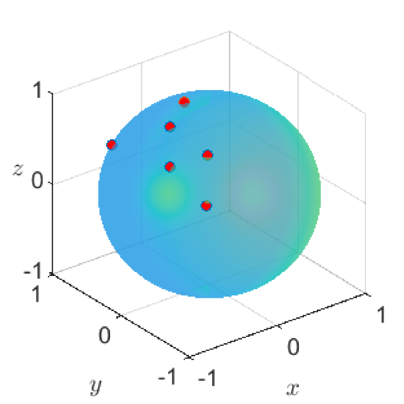
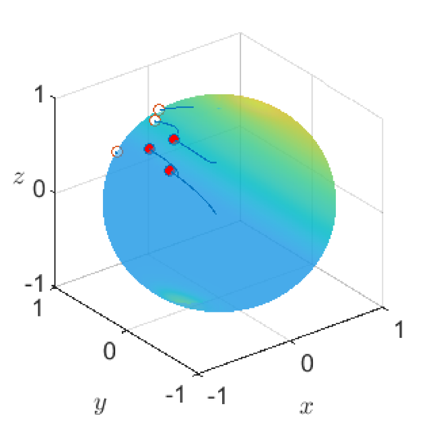
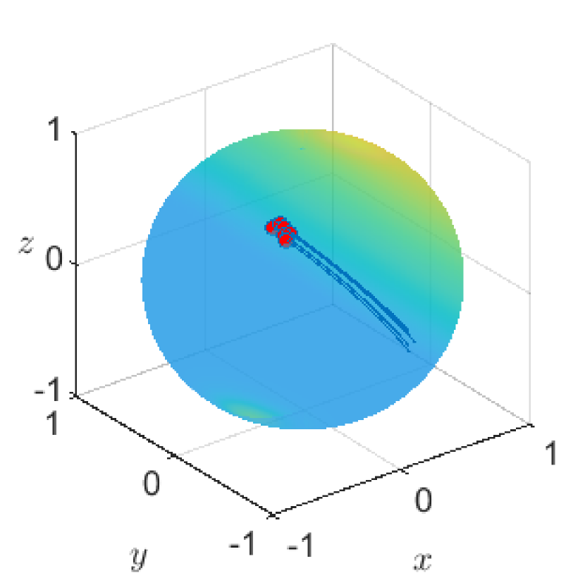
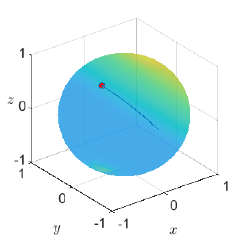
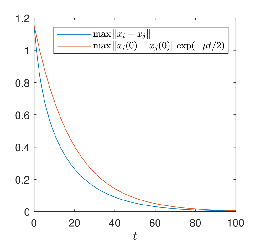
In this section, we conduct some numerical simulations of -agents system of (1.1) to confirm our mathematical results in Theorem 1 and to check the exponential convergence rate
We use the fourth order Runge-Kutta method and MATLAB programming for the simulations.
(a)
(b)

(c)
(d)

(e)
(f)
Let
Then we can easily check that satisfies the condition in -. The initial configuration is randomly chosen satisfying conditions in Theorem 1 such that
and
The time evolution of the solution to (1.1) under the above setting is given in Figure 1. To visually represent the solution, we here use red points for the agent’s positions at and the blue lines for the trajectory of agents on the time interval . Here the white points in Figure 1(b) and (c) mean the agent’s positions on the opposite side of the visible side. Eventually, we can observe the phenomenon in Figure 1 that all the agents gather to one point and they converge into a trajectory orbiting a great circle at a constant speed.
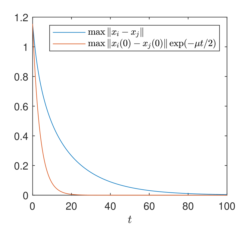
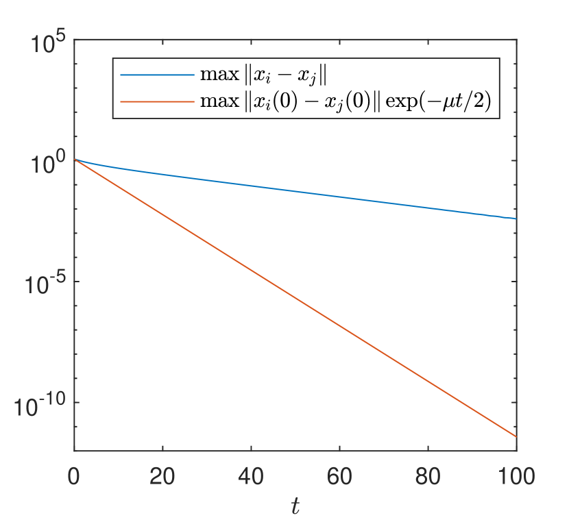
In Figure 2, we display the maximal spatial diameter of the solution and we can check that it decays exponentially as we proved in Theorem 1. Additionally, if we increase the inter-particle bonding force such as , then the above initial data does not satisfy the admissible condition, i.e.,
(a)
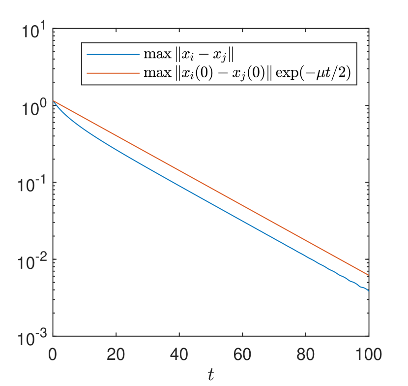
(b) Semi-log graph of (a)
(a)
(b) Semi-log graph of (a)
Then, we can see that the sufficient exponential decay rate does not appear. See Figure 3.
6. conclusion and discussion
In this paper, we studied the interactions of the inter-particle bonding forces and flocking operator on a sphere. We show that the model has the complete position flocking for an admissible initial condition depending on , . We note that the initial data condition does not depend on the number of particles . As the flat space case, we obtain that the ensemble converges to one point particle with one velocity when a flocking model has the inter-particle bonding forces. We crucially use the energy dissipation property in Proposition 2.7 because our model has no momentum conservation. From the energy dissipation leads to uniform upper bound of velocities. We simultaneously use the Lyapunov functional method and a reduction to a linearized system of differential equations to obtain the asymptotic position alignment result.
Acknowledgments
S.-H. Choi is partially supported by NRF of Korea (no. 2017R1E1A1A03070692) and Korea Electric Power Corporation(Grant number: R18XA02).
References
- [1] Abdessameud, A., and Tayebi, A. (2010). On consensus algorithms for double-integrator dynamics without velocity measurements and with input constraints. Systems & Control Letters, 59(12), 812-821.
- [2] Abdessameud, A., and Tayebi, A. (2013). On consensus algorithms design for double integrator dynamics. Automatica, 49(1), 253-260.
- [3] Adler J. (1966). Chemotaxis in bacteria. Science.
- [4] Ando, H., Oasa, Y., Suzuki, I., and Yamashita, M. (1999). Distributed memoryless point convergence algorithm for mobile robots with limited visibility. IEEE Transactions on Robotics and Automation, 15(5), 818-828.
- [5] Bahloul, N. E.H. , Boudjit, S., A., M. and Boubiche, D.E. (2018). A flocking-based on demand routing protocol for unmanned aerial vehicles. Journal of Computer Science and Technology, 33, 263-276.
- [6] Carroll, S.M.: Lecture notes on general relativity. arXiv preprint gr-qc/9712019, 1997.
- [7] Chandler, P. R., Pachter, M., Rasmussen, S. (2001). UAV cooperative control. In Proceedings of the 2001 American Control Conference (Cat. No. 01CH37148), 50-55.
- [8] Chi, D., Choi, S.-H. and Ha, S.-Y. (2014). Emergent behaviors of a holonomic particle system on a sphere. Journal of Mathematical Physics, 55(5), 052703.
- [9] Choi, S.-H., Kwon, D. and Seo, H. (2020). Cucker-Smale type flocking models on a sphere. arXiv preprint arXiv:2010.10693. https://arxiv.org/abs/2010.10693
- [10] Choi, S.-H., Kwon, D. and Seo, H.: Flocking formation and stabilizer of boosted cooperative control on a sphere, preprint.
- [11] Cimino, M. G. C. A. , Lazzeri, A. and Vaglini, G. (2015). Combining stigmergic and flocking behaviors to coordinate swarms of drones performing target search. 2015 6th International Conference on Information, Intelligence, Systems and Applications.
- [12] Cucker, F. and Smale, S. (2009). Emergent Behavior in Flocks. IEEE Transactions on Automatic Control, 52(5), 852–862.
- [13] DeGroot, M. H. (1974). Reaching a consensus. Journal of the American Statistical Association, 69(345), 118-121.
- [14] do Carmo, M.P. (2016). Differential Geometry of Curves and Surfaces. Revised and Updated Second Edition. Courier Dover Publications.
- [15] Eich-Soellner, E. and Führer, C. (1998). Numerical methods in multibody dynamics, vol 45. Springer.
- [16] Flocchini, P., Prencipe, G., Santoro, N., and Widmayer, P. (2005). Gathering of asynchronous robots with limited visibility. Theoretical Computer Science, 337(1-3), 147-168.
- [17] Hairer, E. (2011). Solving differential equations on manifolds. Lecture Notes, Universite de Geneve, Geneva, Switzerland.
- [18] Kuramoto, Y. (1975). International symposium on mathematical problems in theoretical physics. Lecture notes in Physics.
- [19] Lageman, C., and Sun, Z. (2016). Consensus on spheres: Convergence analysis and perturbation theory. In 2016 IEEE 55th Conference on Decision and Control (CDC), 19-24.
- [20] Lee, J. M. (2006). Riemannian Manifolds. An Introduction to Curvature. Springer Science & Business Media.
- [21] Li, W. and Spong, M. W. (2013). Unified cooperative control of multiple agents on a sphere for different spherical patterns. IEEE Transactions on Automatic Control, 59(5), 1283-1289.
- [22] Lin, Z., Francis, B., and Maggiore, M. (2007). State agreement for continuous-time coupled nonlinear systems. SIAM Journal on Control and Optimization, 46(1), 288-307.
- [23] Lohe, M.A. (2009). Non-abelian kuramoto models and synchronization. Journal of Physics A: Mathematical and Theoretical, 42, 395101.
- [24] McGlinn, W. D. (2003). Introduction to Relativity. JHU Press.
- [25] Miao, Y. Q., Khamis, A. and Kamel, M. S. (2010). Applying anti-flocking model in mobile surveillance systems. In 2010 International Conference on Autonomous and Intelligent Systems, AIS 2010, 1-6.
- [26] Murray, R. M. (2007). Recent research in cooperative control of multivehicle systems. Journal of Dynamic Systems, Measurement, and Control, 129(5), 571-583.
- [27] Olfati-Saber, R. (2006). Flocking for multi-agent dynamic systems: Algorithms and theory. IEEE Transactions on automatic control, 51(3), 401-420.
- [28] Park, J., Kim, H. J., and Ha, S.-Y. (2010). Cucker-Smale flocking with inter-particle bonding forces. IEEE Transactions on Automatic Control, 55(11), 2617-2623.
- [29] Ren, W., Beard, R. W., and Atkins, E. M. (2005). A survey of consensus problems in multi-agent coordination. In Proceedings of the 2005, American Control Conference, 1859-1864.
- [30] Ren, W. and Beard, R. W. (2008). Distributed consensus in multi-vehicle cooperative control. Vol. 27. Springer London.
- [31] Rodriguez-Angeles, A., and Nijmeijer, H. (2004). Mutual synchronization of robots via estimated state feedback: a cooperative approach. IEEE Transactions on control systems technology, 12(4), 542-554.
- [32] Schutz, B. F. (1985). A First Course in General Relativity. Cambridge University Press.
- [33] Semnani, S. H. and Basir, O. A. (2014). Semi-flocking algorithm for motion control of mobile sensors in large-scale surveillance systems. IEEE transactions on cybernetics, 45(1), 129-137.
- [34] Spivak, M. (1970). A comprehensive introduction to differential geometry. Vol. I. Publish or Perish, Inc., Wilmington, Del., second edition.
- [35] Spivak, M. (1970). A comprehensive introduction to differential geometry. Vol. II. Publish or Perish, Inc., Wilmington, Del., second edition.
- [36] Talman, R. (2008). Geometric Mechanics. John Wiley & Sons.
- [37] Toner, J. and Tu, Y. (1998). Flocks, herds, and schools: A quantitative theory of flocking. Physical review E, 58, 4828.
- [38] Winfree, A. T. (1967). Biological rhythms and the behavior of populations of coupled oscillators. Journal of theoretical biology, 16(1), 15-42.