Unified Investigation of Rapid Hall Coefficient Changes in Cuprates: Pseudogap and Fermi Surface Influences

We start with a single-band Hubbard model on the 2D square lattice. The Hamiltonian is

$$\hat{H}=-\sum_{\langle i,j\rangle}\sum_{\sigma}\left(t_{ij}\hat{c}^{\dagger}_{i\sigma}\hat{c}_{j\sigma}+h.c.\right)+U\sum_{i}\hat{n}_{i\uparrow}\hat{n}_{i\downarrow},$$

(1)

where $t_{ij}$ denotes the hopping amplitude between lattice site $i$ and $j$ and $U$ represents the strength of the on-site Coulomb interaction. $\hat{c}^{\dagger},\hat{c}$ are electron creation and annihilation operators, respectively. The index $\sigma=\uparrow,\downarrow$ describes the spin orientation. The hopping amplitudes have been investigated theoretically using density-functional-theory calculations [andersen_lda_nodate, pavarini_band-structure_2001, Imada_ab_initio_2022], and experimentally by angle-resolved photoemission spectroscopy (ARPES) [Shen_electronic_1995, Borisenko_joys_2000]. Nearest, second nearest, and third nearest neighbor hopping $t,t^{\prime},t^{\prime\prime}$ are usually taken into account and the former is adopted as the unit of energy. For $\mathrm{La}_{2-x}\mathrm{Sr}_{x}\mathrm{CuO}_{4}$ ($\mathrm{LSCO}$), $t^{\prime}/t\sim-0.1$ while for $\mathrm{YBa}_{2}\mathrm{Cu}_{3}\mathrm{O}_{y}$ ($\mathrm{YBCO}$) and $\mathrm{Bi_{2}Sr_{2}CaCu_{2}O_{8+\delta}}$, $t^{\prime}/t\sim-0.3$. In our calculations, we take $t^{\prime}=-0.25t,t^{\prime\prime}=0.10t$ and a pretty strong $U=6t$, near the typical values presented in literature [mitscherling_longitudinal_2018, Huang_strange_2019]. Taking the lattice constant $a$ as the unit of length, and the energy dispersion without $U$ (i.e., $U=0$) is

	$\displaystyle\epsilon(\vec{k})=$	$\displaystyle-2t\left(\cos k_{x}+\cos k_{y}\right)+4|t^{\prime}|\cos k_{x}\cos k_{y}$		(2)
		$\displaystyle-2t^{\prime\prime}\left(\cos 2k_{x}+\cos 2k_{y}\right).$

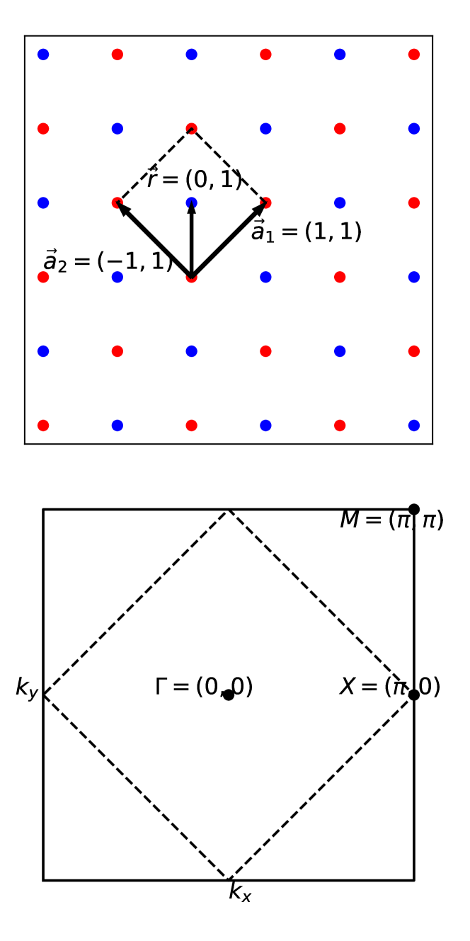
The Hartree-Fock approximation shows that the Hubbard model exhibits a rich phase diagram [Igoshev_Incommensurate_2010, Laughlin_Hartree-Fock_2014, Scholle_comprehensive_2023], considering both magnetic and charge fluctuations. Given the prominence of antiferromagnetic (AF) fluctuations near half-filling, one may expect the magnetic phase transition would capture its key features. For simplicity, we employ a paramagnetic(PM)-AF transition. Both phases could be described in a unified form [Kao_Unified_2023]. When adjacent sites are considered distinctly, the system exhibits a $\sqrt{2}\times\sqrt{2}$ super-lattice with lattice vectors $\vec{a}_{1}=(1,1)$ and $\vec{a}_{2}=(-1,1)$. Within each super-cell, there exist two sites, denoted as $\vec{r}^{A}=(0,0)$ and $\vec{r}^{B}=(0,1)$. The first Brillouin zone is folded accordingly as shown in Figure 1. Kinetic term of Hamiltonian written in basis $\{\psi^{A}_{\uparrow},\psi^{B}_{\uparrow},\psi^{A}_{\downarrow},\psi^{B}_{\downarrow}\}$ is blocked diagonal.

$$\hat{H}_{0,\uparrow}(\vec{k})=\begin{bmatrix}\epsilon_{1}(\vec{k})&\epsilon_{2}(\vec{k})e^{+\mathrm{i}\varphi(\vec{k})}\\ \epsilon_{2}(\vec{k})e^{-\mathrm{i}\varphi(\vec{k})}&\epsilon_{1}(\vec{k})\end{bmatrix},$$

(3)

$$\begin{gathered}\epsilon_{1}(\vec{k})=4|t^{\prime}|\cos k_{x}\cos k_{y}-2t^{\prime\prime}\left(\cos 2k_{x}+\cos 2k_{y}\right),\\ \epsilon_{2}(\vec{k})=-2t\left(\cos k_{x}+\cos k_{y}\right),\\ \varphi(\vec{k})=\vec{k}\cdot\vec{r}^{B}=k_{y}.\end{gathered}$$

(4)

The Hartree-Fock Green’s functions can be expressed by the local densities $n^{A}_{\uparrow},n^{A}_{\downarrow},n^{B}_{\uparrow},n^{B}_{\downarrow}$ from Dyson-Schwinger equation,

$$G^{-1}_{\upuparrows}(k)=\begin{bmatrix}\mathrm{i}\omega_{n}+\mu-Un^{B}_{\uparrow}&0\\ 0&\mathrm{i}\omega_{n}+\mu-Un^{A}_{\uparrow}\end{bmatrix}-H_{0,\uparrow}(\vec{k}).$$

(5)

For the AF phase, they are related to each other $n^{A}_{\uparrow}=n^{B}_{\downarrow},n^{A}_{\downarrow}=n^{B}_{\uparrow}$; for the PM phase, they are all equal. Self-consistent equations are derived by Matsubara sum $\frac{1}{\beta N}\sum_{k}G^{AA}_{\upuparrows}(k)=n^{A}_{\uparrow}$, here $k=(\mathrm{i}\omega_{n},\vec{k})$, and $\beta,N$ denotes inverse of temperature and number of sites, respectively.

Scattering due to interaction plays a pivotal role in cuprates transport property, and it leads us to compute the self-energy with a finite imaginary part at the two-loop level. Making use of standard perturbation theory, we get the perturbation correction to Gaussian approximation (PCGA) [Kao_Unified_2023]. Self-energy $\Sigma_{\upuparrows}(k)$ turns out to be

$$\Sigma^{ab}_{\upuparrows}(k)=-\frac{U^{2}}{\beta^{2}N^{2}}\sum_{q_{1},q_{2}}G^{ba}_{\downdownarrows}(q_{1}+q_{2}-k)G^{ab}_{\upuparrows}(q_{1})G^{ab}_{\downdownarrows}(q_{2}),$$

(6)

where $a,b\in\{A,B\}$. We would see that the real-frequency self-energy $\Sigma_{\upuparrows}(\omega,\vec{k})$ do have a spatially varying imaginary part.

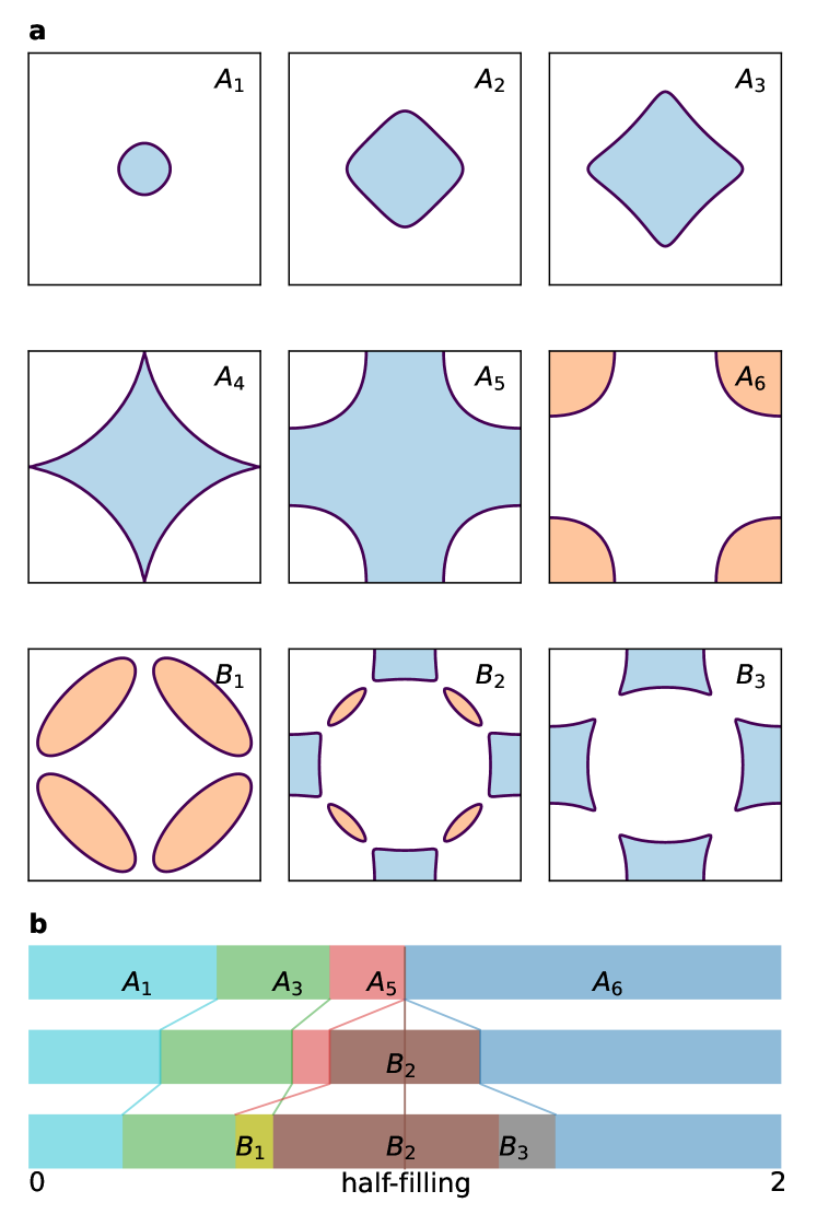
Various methods exist for studying phase transitions in electronic systems, one of which involves detecting the evolution of the Fermi surface (FS). [storey_hall_2016, armitage_angle-resolved_2003, matsui_evolution_2007, louis_remarkable_2019]. Figure 2a shows the evolution of the FS as a function of density, which is determined using the Hartree-Fock approximation.

For the PM phase, in the dilute limit, the FS is nearly a circle, which is convex everywhere. As the electron density grows, the FS around nodal point $(q,q)$ gradually becomes concave ($A_{1}$ to $A_{3}$ in Fig. 2a). The point that FS transition from convex to concave is regarded as Fermi liquid starting to break down [FS_Gindikin_2024]. When anti-nodal point goes to $(\pi,0)$ the topological of FS changes ($A_{4}$ in Fig. 2a).

The AF phase is more complicated since there are finite magnetic moments $m$. Near half-filling, electron pockets and hole pockets coexist as $B_{2}$ in Fig. 2a. With hole/electron doping increases, electron/hole pockets become smaller, and even disappear under some parameter regions. These topological changes also indicate phase boundaries. The boundary ends in high temperature which does not allow the AF phase in corresponding doped levels (between mid- and lower- temperature in Fig. 2b).

To calculate the Hall number, we need to evaluate longitudinal and Hall conductivity respectively. For mean-field theory with magnetic order and uniform scattering rate, there are some systematic researches [Eberlein_2016, mitscherling_longitudinal_2018]. We would derive the formula in a similar way without a uniform scattering rate assumption. Under electromagnetic field, we need to apply Peierls substitution [peierls_zur_1933, wannier_dynamics_1962, Vucice_electrical_2021] to Hamiltonian Equation (1)

$$t_{ij}[\vec{A}]=t_{ij}\exp\left(\mathrm{i}\left(\vec{A}_{i}+\vec{A}_{j}\right)\cdot(\vec{r}_{i}-\vec{r}_{j})/2\right),$$

(7)

where $\vec{A}$ is the vector potential of the electromagnetic field. The current operator $\hat{j}^{\alpha}$ and corresponding bare vertex $\gamma^{\alpha}$ satisfy

$$\hat{j}^{\alpha}(\vec{r})=\left.\frac{\delta\hat{H}[\vec{A}]}{\delta A_{\alpha}(\vec{r})}\right|_{\vec{A}\equiv 0}=\sum_{\vec{r}_{1},\vec{r}_{2}}\sum_{\sigma}c^{\dagger}_{\sigma}(\vec{r}_{1})\gamma^{\alpha}(\vec{r}_{1},\vec{r}_{2};\vec{r})c_{\sigma}(\vec{r}_{2}).$$

(8)

To connect (Hall) conductivity and current-correlation functions, we need to extend linear response theory up to the second order. The coefficients $\Pi$s can be expressed by either correlation functions or conductivity, serving as a bridge between them.

	$\displaystyle\langle j^{\alpha}(\tau,\vec{r})\rangle=$	$\displaystyle\int_{0}^{\beta}\mathrm{d}\tau^{\prime}\ \Pi^{ab}(\tau,\vec{r};\tau^{\prime})A^{E}_{b}(\tau^{\prime})$		(9)
	$\displaystyle+$	$\displaystyle\int_{0}^{\beta}\mathrm{d}\tau^{\prime}\sum_{\vec{r}^{\prime}}\Pi^{abc}(\tau,\vec{r}^{\prime};\tau^{\prime},\vec{r}^{\prime})A^{E}_{b}(\tau^{\prime})A^{B}_{c}(\vec{r}^{\prime})$
	$\displaystyle+$	$\displaystyle\text{higher order response},$

where $a,b,c\in\{x,y,z\}$ denotes spatial components, $\tau$ is the imaginary time and $\vec{A}(\tau,\vec{r})=\vec{A}^{E}(\tau)+\vec{A}^{B}(\vec{r})$. Suppose $\vec{E}(\tau)=E(\tau)\hat{e}_{x},\vec{B}(\vec{r})=B(\vec{r})\hat{e}_{z}$, we could select appropriate gauge to make $\vec{A}^{B}$ in $y$-direction.

$$\left\{\begin{aligned} \langle j^{x}(\tau,\vec{r})\rangle=&\int_{0}^{\beta}\mathrm{d}\tau\ \Pi^{xx}(\tau,\vec{r};\tau^{\prime})A^{E}(\tau^{\prime})\\ \langle j^{y}(\tau,\vec{r})\rangle=&\int_{0}^{\beta}\mathrm{d}\tau\sum_{\vec{r}^{\prime}}\Pi^{yxy}(\tau,\vec{r};\tau^{\prime},\vec{r}^{\prime})A^{E}(\tau^{\prime})A^{B}(\vec{r}^{\prime})\\ E(\tau)=&-\partial_{\tau}A^{E}(\tau),\quad B(\vec{r})=\partial_{x}A^{B}(\vec{r})\end{aligned}\right.$$

(10)

The longitudinal and Hall conductivity $\sigma,\sigma_{\mathrm{Hall}}$ are described by the current response to homogeneous static electric and magnetic fields,

$$j^{x}=\sigma E,\quad j^{y}=\sigma_{\mathrm{Hall}}BE.$$

(11)

And we get $\Pi$s expressed by frequency-dependent conductivity [Voruganti_conductivity_1992]

$$\begin{gathered}\sigma(\omega)=\frac{1}{\mathrm{i}\omega}\left(\Pi^{xx}(\omega,\vec{k}=\vec{0})-(\omega\to 0)\right),\\ \sigma_{\mathrm{Hall}}(\omega)=\frac{1}{\omega}\frac{\partial}{\partial k_{x}}\left(\Pi^{yxy}(\omega,\vec{k}=\vec{0})-(\omega\to 0)\right).\end{gathered}$$

(12)

By definition, static limit $\sigma=\sigma(\omega=0),\sigma_{\mathrm{Hall}}=\sigma_{\mathrm{Hall}}(\omega=0)$. Our supercells with $A,B$ sites break translation invariance, so $\Pi$s in momentum space should be symmetrized as

	$$\displaystyle\Pi^{xx}(\vec{k})=\frac{1}{N}\sum_{\vec{r}}e^{-\mathrm{i}\vec{k}\cdot\vec{r}}\Pi^{xx}(\vec{r}),$$		(13)
	$$\displaystyle\Pi^{yxy}(\vec{k})=\frac{1}{N^{2}}\sum_{\vec{r}_{1},\vec{r}_{2}}e^{-\mathrm{i}\vec{k}\cdot(\vec{r}-\vec{r}_{2})}\Pi^{xx}(\vec{r}_{1},\vec{r}_{2}).$$		(14)

On the other hand, in the language of path-integral, the expectation value of current can be expressed by action including electromagnetic field $S[\psi^{*},\psi;\vec{A}]$

$$\langle j^{\alpha}(\tau,\vec{r})\rangle=-\frac{\delta}{\delta A_{\alpha}(\tau,\vec{r})}\ln\int D[\psi^{*},\psi]\ e^{-S[\psi^{*},\psi;\vec{A}]}.$$

(15)

Furthermore, take the derivative of $\vec{A}$ by Eq. (9). Since conductivity only relate to derivative of $\Pi^{xx}$ and $\Pi^{yxy}$ as Eq. (12), any terms with $\delta(\tau,\tau^{\prime})$ or $\delta(r_{x},r^{\prime}_{x})$ could be dropped.

	$\displaystyle\Pi^{xx}(\tau,\vec{r};\tau^{\prime})=$	$\displaystyle\sum_{\vec{r}^{\prime}}\left\langle j^{x}(\tau,\vec{r})j^{x}(\tau^{\prime},\vec{r}^{\prime})\right\rangle_{c}+\left\langle\frac{\delta j^{x}(\tau,\vec{r})}{\delta A^{E}(\tau^{\prime})}\right\rangle\to\sum_{\vec{r}^{\prime}}\left\langle j^{x}(\tau,\vec{r})j^{x}(\tau^{\prime},\vec{r}^{\prime})\right\rangle_{c},$		(16)
	$\displaystyle\Pi^{yxy}(\tau,\vec{r};\tau^{\prime},\vec{r}^{\prime})=$	$\displaystyle\int\mathrm{d}\tau^{\prime\prime}\sum_{\vec{r}^{\prime\prime}}\ \left\langle j^{y}(\tau,\vec{r})j^{x}(\tau^{\prime},\vec{r}^{\prime\prime})j^{y}(\tau^{\prime\prime},\vec{r}^{\prime})\right\rangle_{c}+\int\mathrm{d}\tau^{\prime\prime}\ \left\langle\frac{\delta j^{y}(\tau,\vec{r})}{\delta A^{E}(\tau^{\prime})}j^{y}(\tau^{\prime\prime},\vec{r}^{\prime})\right\rangle_{c}$
	$\displaystyle+$	$\displaystyle\sum_{\vec{r}^{\prime}}\left\langle\frac{\delta j^{y}(\tau,\vec{r})}{\delta A^{B}(\vec{r}^{\prime})}j^{x}(\tau^{\prime},\vec{r}^{\prime\prime})\right\rangle_{c}+\sum_{\vec{r}^{\prime\prime}}\ \left\langle j^{y}(\tau,\vec{r})\frac{\delta j^{x}(\tau^{\prime},\vec{r}^{\prime\prime})}{\delta A^{B}(\vec{r}^{\prime})}\right\rangle_{c}+\left\langle\frac{\delta^{2}j^{y}(\tau,\vec{r})}{\delta A^{B}(\vec{r}^{\prime})\delta A^{E}(\tau^{\prime})}\right\rangle$
	$\displaystyle\to$	$\displaystyle\int\mathrm{d}\tau^{\prime\prime}\sum_{\vec{r}^{\prime\prime}}\ \left\langle j^{y}(\tau,\vec{r})j^{x}(\tau^{\prime},\vec{r}^{\prime\prime})j^{y}(\tau^{\prime\prime},\vec{r}^{\prime})\right\rangle_{c}+\sum_{\vec{r}^{\prime\prime}}\ \left\langle j^{y}(\tau,\vec{r})\frac{\delta j^{x}(\tau^{\prime},\vec{r}^{\prime\prime})}{\delta A^{B}(\vec{r}^{\prime})}\right\rangle_{c}.$

Here $\langle\cdot\rangle_{c}$ denotes connected correlation functions. The lowest order of $\Pi^{yxy}$ consists $3$ Feynman diagrams as Fig. LABEL:fig:3. Bare vertices are derivatives of Hamiltonian like Eq. (8)

$$\begin{gathered}\left.\frac{\delta\hat{H}[\vec{A}]}{\delta A_{\alpha}(\vec{r})}\right|_{\vec{A}\equiv 0}=\sum_{\vec{r}_{1},\vec{r}_{2}}\sum_{\sigma}c^{\dagger}_{\sigma}(\vec{r}_{1})\gamma^{\alpha}(\vec{r}_{1},\vec{r}_{2};\vec{r})c_{\sigma}(\vec{r}_{2}),\\ \left.\frac{\delta^{2}\hat{H}[\vec{A}]}{\delta A_{\alpha}(\vec{r})\delta A_{\beta}(\vec{r})}\right|_{\vec{A}\equiv 0}=\sum_{\vec{r}_{1},\vec{r}_{2}}\sum_{\sigma}c^{\dagger}_{\sigma}(\vec{r}_{1})\gamma^{\alpha\beta}(\vec{r}_{1},\vec{r}_{2};\vec{r})c_{\sigma}(\vec{r}_{2}).\end{gathered}$$

(17)