Unified first law of thermodynamics in Gauss-Bonnet gravity on an FLRW background

As stated before, the pertinent entity to describe the thermodynamics of the Universe is the so-called apparent horizon ($AH$) Faraoni:2011hf ; Faraoni:2015ula . The $AH$ is the surface satisfying

$$h^{ij}\nabla_{i}R\nabla_{j}R=0,\quad i,j=t,r,$$

(1)

where $R$ is the areal radius defined as $R(t,r)=a(t)r$, being $a(t)$ the scale factor, $r$ the co–moving radial distance and $h^{ij}$ the inverse metric of the two–dimensional metric $h_{ij}$ on the $t-r$ plane. These definitions come from the FLRW line element

$$ds^{2}=-dt^{2}+a^{2}(t)\left(\frac{dr^{2}}{1-kr^{2}}+r^{2}d\Omega_{(n-2)}^{2}\right),$$

(2)

re-expressed by means of the warped product as

$$ds^{2}=h_{ij}dx^{i}dx^{j}+R^{2}d\Omega_{(n-2)}^{2},$$

(3)

where in the above expressions $k=0,\pm 1$ is the spatial curvature and $d\Omega_{(n-2)}^{2}$ is the line element of a $(n-2)$–dimensional unit sphere. Therefore, in this way the metric on $t-r$ plane is given by $h_{ij}=\text{diag}\{-1,a^{2}/\left(1-kr^{2}\right)\}$.

Now, the solution $R_{AH}$ of Eq. (1) is given by¹¹1The apparent horizon in this context, is a dynamical marginally outer trapped surface (MOTS) with vanishing expansion Faraoni:2015ula .Faraoni:2011hf ; Faraoni:2015ula

$$R_{AH}=\frac{1}{\sqrt{H^{2}+\frac{k}{a^{2}}}},$$

(4)

with $H=\dot{a}/a$ being the Hubble’s parameter. For a flat FLRW, when $k=0$, the expression (4) coincides with the Hubble’s radius. From now on, we will keep the spatial curvature $k$ arbitrary.

Although the co-moving patch²²2Greeks indexes run over the full space-time components, Latin indexes only run over time and radial components. $x^{\mu}=\{t,r,\theta_{1}\ldots\theta_{n-2}\}$, with $n-3$ angles ranging over $[0,\pi]$ and $n-2$ ranging over $[0,2\pi)$, is the natural chart for the FLRW metric, it is more instructive to express this model using the Schwarzschild–like coordinate chart $y^{\mu}=\{T,R,\theta_{1}\ldots\theta_{n-2}\}$. One must establish the relation between the co-moving time $t$ and radius $r$ with the new time $T$ and radius $R$ coordinates to do this. These relations are given by Faraoni:2011hf ; Faraoni:2015ula ; Nielsen:2005af

$$dt=FdT-\beta dR,$$

(5)

$$dr=-\frac{HRF}{a}dT+\frac{1}{a}dR,$$

(6)

where $F=F(T,R)$ is an integration factor in order to assure that $dt$ being an exact differential, $H$ and $a$ implicit functions of the time coordinate $T$ and $\beta$ a function given by

$$\beta(t,R)=\frac{HR}{1-H^{2}R^{2}-kr^{2}}.$$

(7)

In this way, the line element (2) acquires the following form

$$\begin{split}ds^{2}=-\left(1-\frac{H^{2}R^{2}}{1-kR^{2}/a^{2}}\right)F^{2}dT^{2}&\\ +\frac{dR^{2}}{1-kR^{2}/a^{2}-H^{2}R^{2}}+R^{2}d\Omega_{(n-2)}^{2}.\end{split}$$

(8)

From (8) it is easy to get the $AH$ by solving

$$g^{RR}=0,$$

(9)

for $R$ leading as before to (4).

As it is well-known, there is no preferred time coordinate in an evolving time-dependent space-time. This is because there is no asymptotically time–like a Killing vector field. Then, to bypass this issue, a divergence-free vector field which is present in any time-dependent spherically symmetric³³3For generalizations of the Kodama vector to symmetries other than the spherical one see for example Tung:2007vq ; Kinoshita:2021qsv . space-time was introduced in Kodama:1979vn and is referred as the Kodama vector field. The Kodama vector field identifies a natural time-like direction and is used to define locally conserved currents Kodama:1979vn ; Hayward:1993wb . So, for dynamical situations, it is necessary to introduce or replace the objects used in a static/stationary context for those giving the proper description Hayward:1997jp , that is

1. 1.

   Killing vector field $\mapsto$ Kodama vector field.

2. 2.

   Killing horizon $\mapsto$ apparent horizon.

In general, the Kodama vector field is defined as

$$K^{i}\equiv E^{ij}\nabla_{j}R,$$

(10)

where $E^{ij}$ is the skew-symmetric Levi–Civita tensor defines as

$$E^{i_{1}\ldots i_{n}}=\frac{\text{sgn}\left(|h|\right)}{\sqrt{|h|}}\varepsilon^{i_{1}\ldots i_{n}},$$

(11)

where $h$ is the determinant of the metric $h_{ij}$, the sign function $\text{sgn}(h)=(-1)^{q}$, with $q$ the number of negatives in the metric signature⁴⁴4This definition occurs when the metric has an odd number of negative signs in the signature as in our case. and $\varepsilon^{i_{1}\ldots i_{n}}$ the standard Levi–Civita symbol defined according our basis coordinate orientation as

$$\varepsilon_{i_{1}\ldots i_{n}}=-\varepsilon^{i_{1}\ldots i_{n}}\left\{\begin{aligned} +1&\text{ even permutation, }\\ -1&\text{ odd permutation, }\\ 0&\text{ otherwise. }\end{aligned}\right.$$

(12)

On the other hand, if the metric is expressed in Schwarzschild–like coordinate gauge, the components of the Kodama vector (10) assume the simple form Kodama:1979vn ; Racz:2005pm

$$K^{i}=\frac{1}{\sqrt{g_{TT}g_{RR}}}\left(\frac{\partial}{\partial t}\right)^{i}.$$

(13)

Then, for the line element (8) one gets

$$K=K^{T}\partial_{T}=F\sqrt{1-\frac{k}{a^{2}}R^{2}}\,\partial_{T}.$$

(14)

Now, from the norm of the Kodama vector $K^{2}=K_{i}K^{i}$

$$K^{2}=K_{i}K^{i}=-\left(1-H^{2}R^{2}-\frac{kR^{2}}{a^{2}}\right)=-\left(1-\frac{R^{2}}{R_{AH}^{2}}\right),$$

(15)

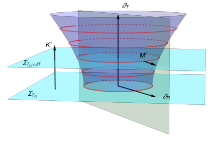
we can infer the following valuable information: the Kodama vector is time–like if $K^{2}<0$, thus $R<R_{{AH}}$, null $K^{2}=0$ if $R=R_{{AH}}$ and space–like if $K^{2}>0$, that is, outside the $AH$ $R>R_{{AH}}$. Thus, the $AH$ behaves as a null surface in this case. Fig. 1 shows a schematic representation of the Kodama vector (14). As can be appreciated, in the chart $y^{\mu}=\{T,R,\theta_{1}\ldots\theta_{n-2}\}$ it is hypersurface orthogonal to the Cauchy hyper–surface $\Sigma(R,\theta_{1}\ldots\theta_{n-2}):T-T_{0}=0$. This fact is clear from the general hyper–orthogonal condition, which reads: $X_{i}=\Lambda(x^{j})\nabla_{i}\Sigma$, being $\Lambda$ some proportionality factor, which in general will vary from point to point and $\nabla_{i}\Sigma=\partial_{T}$. Besides, the Kodama vector is orthogonal to the two–spheres of symmetry. Interestingly, the modulus of the norm (15) coincides with the space–like slice of marginally trapped tube (MTT) given by⁵⁵5As we are performing a foliation of the space-time, as shown in Fig. 1, the surface $\chi$ is just a two-sphere of radius $R_{AH}$ embedded in a specific Cauchy hypersurface $\Sigma$. However, if we collect all the constant time slices $\Sigma$ one gets the MTT (purple surface in Fig. 1), equivalently if one considers $\chi(T,\theta_{1}\ldots\theta_{n-2})$ instead of only $\chi(\theta_{1}\ldots\theta_{n-2})$ one obtains the full MTT.

$$\chi(\theta_{1}\ldots\theta_{n-2}):1-\frac{R^{2}}{R^{2}_{AH}}=0.$$

(16)

It is worth mentioning that each space–like slice (red circles) defines the MOTS given rise to the $AH$ Faraoni:2011hf ; Faraoni:2015ula .

In analogy with Killing vectors, the Kodama vector satisfies

$$\frac{1}{2}h^{ij}K^{k}\left(\nabla_{k}K_{i}-\nabla_{i}K_{k}\right)=\kappa_{\text{Kodama }}K^{j},$$

(17)

where $\nabla_{i}$ is covariant the derivative compatible with the metric $h_{ij}$ ($\nabla_{k}h_{ij}=0$). The Eq. (17) defines the notion of surface gravity for dynamical scenarios. Usually, this is referred to as the Hayward–Kodama (HK) surface gravity Hayward:1997jp , which in general has the following expression independent of the gravitational theory at hand

$$\kappa_{\text{HK }}=\frac{1}{2\sqrt{|h|}}\partial_{i}\left(\sqrt{|h|}h^{ij}\partial_{j}R\right).$$

(18)

Now, we can discuss the thermodynamics of the FLRW space-time (2) through the associated thermodynamics UFL in the context of the higher dimensional GB theory.

The whole action of the $n$–dimensional GB⁶⁶6This theory is also known as Einstein-Gauss-Bonnet (EGB) gravity; however, we will refer to this theory as GB only. couple to matter fields, is given by

$$S_{GB}=\frac{1}{16\pi G_{n}}\int_{\mathcal{M}}d^{n}x\sqrt{-g}\left[\mathcal{R}+\alpha\mathcal{G}_{\text{GB}}\right]+\text{B.T.}+S_{m},$$

(19)

where $\mathcal{R}$ is the $n$–dimensional Ricci scalar, B.T. stands for boundary terms in order to have a well–defined action principle, $G_{n}$ the $n$–dimensional gravitational constant, $\alpha$ is a constant with units of length squared and $S_{m}$ is the action of the matter fields. The GB term $\mathcal{G}_{GB}$ reads as

$$\mathcal{G}_{\text{GB}}=R^{2}-4R^{\mu\nu}R_{\mu\nu}+R^{\mu\nu\sigma\gamma}R_{\mu\nu\sigma\gamma}.$$

(20)

It is worth mentioning that, in the case of superstring theory, in the low energy limit, $\alpha$ is related to the inverse string tension and is positive definite Gross:1986iv ; Gross:1986mw . Besides, the GB action is a natural extension of the Einstein theory in that no derivatives higher than second order appear in the field equations. For this to happen, the numerical coefficient of the $\mathcal{G}_{GB}$ must be $\{1,-4,1\}$ as shown in Eq. (20).

Now, taking variations with respect to metric tensor $g^{\mu\nu}$, the field equations coming from the action (19) are given by

$$G^{\mu}_{\nu}+\alpha H^{\mu}_{\nu}=8\pi G_{n}T^{\mu}_{\nu},$$

(21)

being

$$G_{\mu\nu}=R_{\mu\nu}-\frac{1}{2}g_{\mu\nu}\mathcal{R},$$

(22)

the Einstein tensor and

	$\displaystyle H_{\mu\nu}$	$\displaystyle=2\left(\mathcal{R}R_{\mu\nu}-2R_{\mu\lambda}R_{\nu}^{\lambda}-2R^{\gamma\delta}R_{\gamma\mu\delta\nu}+R_{\mu}^{\alpha\gamma\delta}R_{\alpha\nu\gamma\delta}\right)$		(23)
		$\displaystyle-\frac{1}{2}g_{\mu\nu}\mathcal{G}_{GB}$

the contribution coming from the GB term (20), the so–called Lanczos tensor. As we know, for $n=4$, the tensor $H_{\mu\nu}$ is zero because the GB term (20) becomes a topological invariant, not affecting the dynamic of the theory. Besides, $T^{\mu}_{\nu}$ is the energy–momentum tensor for matter fields obtained from $S_{m}$.

Next, assuming that the energy-momentum tensor is the one describing an isotropic fluid

$$T_{\mu\nu}=\left(\rho+p\right)X_{\mu}X_{\nu}+pg_{\mu\nu},$$

(24)

where $\rho$ is the density, $p$ the isotropic pressure and $X^{\mu}X_{\mu}=-1$ the four–velocity. The field Eqs. (21) subject to the line element (2) lead to the following Friedmann equations in the GB scenario

$$\frac{1}{R^{2}_{AH}}+\frac{\tilde{\alpha}}{R^{4}_{AH}}=\frac{16\pi G_{n}}{(n-1)(n-2)}\rho,$$

(25)

$$\left(1+2\frac{\tilde{\alpha}}{R^{2}_{AH}}\right)\left(\dot{H}-\frac{k}{a^{2}}\right)=-\frac{8\pi G_{n}}{n-2}(\rho+p).$$

(26)

As expected, the above expressions are modified by the presence of the GB terms throughout the coupling constant $\tilde{\alpha}\equiv(n-3)(n-4)\alpha$ and also by the dimension $n$ of the space-time, recovering the usual Friedmann equations for the GR scenario when $n=4$.

In obtaining the above expressions, we have used Ricci’s scalar

$$\mathcal{R}=6\left(\frac{\dot{a}^{2}}{a^{2}}+\frac{\ddot{a}}{a}+\frac{k}{a^{2}}\right),$$

(27)

and the GB term

$$\mathcal{G}_{\text{GB}}=24\left(\frac{k}{a^{2}}+H^{2}\right)\left(\dot{H}+H^{2}\right).$$

(28)

In general, to deal with the thermodynamics of $AH$s, one needs to modify the usual approach based on the thermodynamics first law, employed in the static/stationary BHs case Bardeen:1973gs ; Bekenstein:1973ur ; Hawking:1975vcx ; Gibbons:1976ue ; York:1986it . Hayward developed this approach in a series of articles Hayward:1993wb ; Hayward:1994bu ; Hayward:1997jp . The main ingredients of this formulation are: i) the Misner–Sharp (MS) mass $M_{AH}$ Misner:1964je , interpreted as the internal energy, ii) the HK surface gravity (18) (related with the temperature horizon) and iii) the areal volume $V_{AH}=\frac{4\pi}{3}R^{3}_{AH}$. Additionally, it is necessary to introduce new quantities to reach the desired thermodynamics description. These quantities are: iv) the density work $W$ and the v) energy–flux $\psi_{i}$ across the $AH$ Hayward:1997jp . Using the metric in the representation given by Eq. (3), the definition of these new pieces is given by

$$W\equiv-\frac{1}{2}h_{ij}T^{ij},$$

(29)

and

$$\psi_{i}\equiv T^{j}_{i}\nabla_{i}R+W\nabla_{i}R,$$

(30)

respectively.

Putting together all these objects, the thermodynamics UFL acquires the following form Hayward:1993wb ; Hayward:1994bu ; Hayward:1997jp

$$\nabla_{i}M=A\psi_{i}+W\nabla_{i}V,$$

(31)

or by identifying the mass $M$ with the internal energy $E$ one obtains

$$\nabla_{i}E=A\psi_{i}+W\nabla_{i}V.$$

(32)

It is worth mentioning that the term $A\psi_{i}$ is called the energy-supply vector.

As stated by Hayward in Hayward:1997jp , the thermodynamics description comes when (32) is projected along the direction of the $AH$, that is,

$$z^{i}\nabla_{i}E=\frac{\kappa_{\text{HK}}}{8\pi}z^{i}\nabla_{i}A+Wz^{i}\nabla_{i}V,$$

(33)

where the following identification has been made $A\psi_{i}=\frac{\kappa_{\text{HK}}}{8\pi}z^{i}\nabla_{i}A$ (see Hayward:1997jp ; Cai:2006rs for further details about how to obtain this identification) and $z^{i}$ is a vector tangent to the $AH$. Interestingly, the Eq. (33) can be re-expressed as

$$\frac{\kappa_{\text{HK}}}{8\pi}z^{i}\nabla_{i}A=R^{n-3}z^{i}\nabla_{i}\left(\frac{E}{R^{n-3}}\right)-Wz^{i}\nabla_{i}V,$$

(34)

where it is argued that the first term on the right-hand member of the above expression becomes zero along the $AH$ Cai:2005ra ; Helou:2015yqa .

In Cai:2005ra ; Akbar:2006kj ; Cai:2006rs , the above statement was employed (in the GR framework) to recognize the left-hand member as the Clausius relation. In this way, the second Friedmann equation is obtained using the corresponding entropy and the temperature identification with the HK surface gravity. Nevertheless, in Binetruy:2014ela ; Helou:2015yqa ; Helou:2015zma , it was shown that these assumptions are not necessary to regain the second Friedmann equation. This is because the term claimed to be zero along the $AH$ is zero for any constant $R$ (including the particular case $R=R_{A}$). Moreover, projecting the remaining terms leads to the desired result without further consideration. The same argument was used in the context of GB gravity Cai:2005ra . Nevertheless, the MS energy (mass) in the GB theory contains additional terms (corrections) Maeda:2006pm ; Maeda:2007uu ; Maeda:2008nz , contributing to the equation of motion (see Eqs. (25)–(26)). Therefore, in the present case, it is not correct to argue that the first term in the right-hand side of Eq. (34) is vanishing along the $AH$ because both the left-hand side and the second term in the right-hand side, are not containing any information about the corrections introduced by the GB term. The only way to assume the above is to set $AH$ to be constant and then assume the Clausius relation. However, this is a strong restriction because the $AH$ is dynamic. Then, to recast Friedmann Eqs. (25)–(26) from the UFL (32) we are going to project it along the Kodama vector direction (leading to Eq. (26)) and along the direction orthogonal to the Kodama vector (obtaining Eq. (25)). It is worth mentioning that the information about the field equations is already contained in (32). Therefore, by projecting it along different directions, we only isolate a particular information about the FLRW dynamic.

To proceed further, we must introduce an essential ingredient: the MS energy for GB theory. In Maeda:2006pm ; Maeda:2007uu ; Maeda:2008nz , the spherically symmetric gravitational collapse of a dust cloud in the GB scenario, where the MS energy Misner:1964je associated with this process was found to be

	$\displaystyle E$	$\displaystyle\equiv\frac{(n-2)\pi^{(n-1)/2}}{8\pi G_{n}\Gamma\left[\frac{(n-1)}{2}\right]}\bigg{[}R^{n-3}\left(1-h^{ij}\nabla_{i}R\nabla_{j}R\right)$		(35)
		$\displaystyle+\tilde{\alpha}R^{n-5}\left(1-h^{ij}\nabla_{i}R\nabla_{j}R\right)^{2}\bigg{]}.$

The MS energy (35) evaluated at the FLRW metric (2) reads

$$E_{\text{FLRW}}=\frac{(n-2)\pi^{(n-1)/2}}{8\pi G_{n}\Gamma\left[\frac{(n-1)}{2}\right]}\frac{R^{n-1}}{R^{2}_{AH}}\left[1+\frac{\tilde{\alpha}}{R^{2}_{AH}}\right].$$

(36)

Of course, the above expressions reduce to the GR for $n=4$.

It should be noted that the UFL (32) was derived using the warped chart (3). As we are working in the Schwarzschild patch (8) where the time $T$ and radial $R$ coordinates are independent coordinates from each one, we need to transform every object of (32) to get the desired result, taking into account that the area $A$, the work density $W$ and the volume $V$ do not transform since they are invariant (scalars). Therefore, for the component of the covariant derivative, one has

	$\displaystyle\nabla_{T}$	$\displaystyle=$	$\displaystyle\frac{\partial t}{\partial T}\nabla_{t}+\frac{\partial r}{\partial T}\nabla_{r}=F\nabla_{t}-\frac{HRF}{a}\nabla_{r},$		(37)
	$\displaystyle\nabla_{R}$	$\displaystyle=$	$\displaystyle\frac{\partial t}{\partial R}\nabla_{t}+\frac{\partial r}{\partial R}\nabla_{r}=-\beta\nabla_{t}+\frac{1}{a}\nabla_{r},$		(38)

while for the energy–flux vector

	$\displaystyle\psi_{T}$	$\displaystyle=$	$\displaystyle\frac{\partial t}{\partial T}\psi_{t}+\frac{\partial r}{\partial T}\psi_{r}=F\psi_{t}-\frac{HRF}{a}\psi_{r},$		(39)
	$\displaystyle\psi_{R}$	$\displaystyle=$	$\displaystyle\frac{\partial t}{\partial R}\psi_{t}+\frac{\partial r}{\partial R}\psi_{r}=-\beta\psi_{t}+\frac{1}{a}\psi_{r},$		(40)

obtaining

	$\displaystyle\psi_{T}$	$\displaystyle=$	$\displaystyle-HRF\left(p+\rho\right),$		(41)
	$\displaystyle\psi_{R}$	$\displaystyle=$	$\displaystyle\frac{1}{2}\left(1-k\frac{R^{2}}{a^{2}}\right)\left(1-\frac{R^{2}}{R^{2}_{AH}}\right)^{-1}\left(p+\rho\right).$		(42)

To get (41) and (42) we used $\psi_{t}=-HR\left(p+\rho\right)/2$ and $\psi_{r}=a\left(p+\rho\right)/2$.

Now, the UFL (32) projected on the Kodama (14) vector yields to

$$K^{T}\nabla_{T}E=AK^{T}\psi_{T}+WK^{T}\nabla_{T}V,$$

(43)

giving

$$\begin{split}K^{T}\nabla_{T}E=-\frac{(n-2)\pi^{(n-1)/2}}{4\pi G_{n}\Gamma\left[\frac{(n-1)}{2}\right]}F^{2}\sqrt{1-\frac{k}{a^{2}}R^{2}}\frac{R^{n-1}\dot{R}_{AH}}{R^{3}_{AH}}&\\ \times\left(1+2\frac{\tilde{\alpha}}{R^{2}_{AH}}\right),\end{split}$$

(44)

$$WK^{T}\nabla_{T}V=0,$$

(45)

$$AK^{T}\psi_{T}=-\frac{2\pi^{(n-1)/2}}{\Gamma\left[\frac{(n-1)}{2}\right]}F^{2}HR^{n-1}\left(p+\rho\right).$$

(46)

Putting together (44), (45) and (46) and after some algebra we obtain

$$\left(1+2\frac{\tilde{\alpha}}{R^{2}_{AH}}\right)\left(\dot{H}-\frac{k}{a^{2}}\right)=-\frac{8\pi G_{n}}{n-2}(\rho+p),$$

(47)

where the following expression has been used in obtaining the above result

$$\dot{R}_{AH}=-HR^{3}_{AH}\left(\dot{H}-\frac{k}{a^{2}}\right),$$

(48)

recalling that every object is an implicit function of the $T$ time coordinate. Thus, the over-dot means differentiation with respect to $T$.

Next, the orthogonal vector to the Kodama vector is given by

$$M=M^{R}\partial_{R}=-\frac{1}{a}\sqrt{1-k\frac{R^{2}}{a^{2}}}\left(1-\frac{R^{2}}{R^{2}_{AH}}-H^{2}R^{2}\right)\partial_{R}.$$

(49)

As can be seen, the vector (49) is tangent to the hypersurface $\Sigma$, thus orthogonal to the Kodama vector (see Fig. 1), and hypersurface orthogonal to the two spheres defining the $AH$ (equivalently hypersurface orthogonal to the (n–2)–dimensional hypersurface (16)). However, it is not a null vector on (16) as the Kodama vector does.

Projecting (32) along the direction of (49) we have

$$\begin{split}M^{R}\nabla_{R}E=-\frac{(n-2)\pi^{(n-1)/2}}{8\pi aG_{n}\Gamma\left[\frac{(n-1)}{2}\right]}\sqrt{1-k\frac{R^{2}}{a^{2}}}&\\ \times\left[1-\frac{R^{2}}{R^{2}_{AH}}-H^{2}R^{2}\right]R^{n-2}&\\ \times\left[1-\frac{R^{2}}{R^{2}_{AH}}\right]^{-1}\bigg{[}-\left(n-1\right)\frac{H^{2}R^{n+2}}{R^{2}_{AH}}&\\ \times\left(1+\frac{\tilde{\alpha}}{R^{2}_{AH}}\right)+\frac{2H\dot{R}_{AH}R^{n+2}}{R^{3}_{AH}}&\\ \times\left(1+2\frac{\tilde{\alpha}}{R^{2}_{AH}}\right)+\frac{\left(n-1\right)}{R^{2}_{AH}}\left(1+\frac{\tilde{\alpha}}{R^{2}_{AH}}\right)&\\ \times\left(1-\frac{R^{2}}{R^{2}_{AH}}\right)\bigg{]},\end{split}$$

(50)

$$\begin{split}WM^{R}\nabla_{R}V=\frac{\pi^{(n-1)/2}}{\Gamma\left[(n-1)/2\right]}\left(1-\frac{R^{2}}{R^{2}_{AH}}\right)^{-1}&\\ \times\left(1-\frac{R^{2}}{R^{2}_{AH}}-H^{2}R^{2}\right)\left(\rho-p\right)R^{n-2},\end{split}$$

(51)

$$\begin{split}AM^{R}\psi_{R}=\frac{\pi^{(n-1)/2}}{\Gamma\left[(n-1)/2\right]}\left(1-\frac{R^{2}}{R^{2}_{AH}}\right)^{-1}&\\ \times\left(1-k\frac{R^{2}}{R^{2}_{AH}}\right)\left(\rho+p\right)R^{n-2}.\end{split}$$

(52)

After some algebra, from expressions (50), (51) and (52) the output is

$$\frac{1}{R^{2}_{AH}}+\frac{\tilde{\alpha}}{R^{4}_{AH}}=\frac{16\pi G_{n}}{(n-1)(n-2)}\rho.$$

(53)

To obtain the first Friedmann Eq. (53) we have used $W=(\rho-p)/2$, $V=\pi^{(n-1)/2}R^{n-1}/\Gamma[(n+1)/2]$, $A=2\pi^{(n-1)/2}R^{n-2}/\Gamma[(n-1)/2]$ and the previous result (51) to cancel out the pressure $p$.

At this stage, some comments are pertinent. First of all, to obtain the Friedmann field equations (51) and (50), it is not necessary to assume from the very beginning the Clausius relation or include the associated entropy and temperature. Secondly, the complete information about the dynamic of the GB theory (in this case) in an FLRW background is already contained in the UFL (32), and its projection on different directions isolates a specific part of it. As the Kodama vector defines a privileged time direction, it leads to a dynamical equation as (51), while along the orthogonal direction with respect to the Kodama flow, the vector (49) provides the equation for the density $\rho$. Although we have not used the Clausius relation and the corresponding GB entropy and temperature to obtain the above result, it does not imply that this relation and associated quantities are not fundamental in the thermodynamical description of gravity Jacobson:1995ab . In what follows, we are to get the GB entropy by identifying the surface gravity (18) with the temperature Bardeen:1973gs ; Hawking:1975vcx ; Bekenstein:1973ur ; Hayward:1993wb ; Hayward:1994bu ; Hayward:1997jp ; Jacobson:1995ab and those terms accompanying it as the entropy variation. After integrating these terms, we will obtain the desired expression for the GB entropy. Of course, to achieve it, one needs to employ (32) as the starting point in conjunction with the on-shell equations of motion.

In the previous subsection III.2, we obtained the dynamic description (equation of motion) for the FLRW space-time in the GB gravity theory. It was reached starting from the thermodynamics UFL (32) and projecting it along different directions concerning the $AH$. In doing this, there was no assumption about temperature and entropy. Notwithstanding, as was proven and established at the starting works Bardeen:1973gs ; Hawking:1975vcx ; Bekenstein:1973ur ; Gibbons:1976ue ; York:1986it ; Jacobson:1995ab , there is a strong connection between the temperature and the surface gravity and also between the entropy and the area of the horizon (whatever the horizon, event or apparent horizons). Therefore, the link gravity $\iff$ thermodynamics becomes evident (see Fig. 2 for a schematic representation of this conjecture).

In this subsection, we want to obtain the entropy for the GB theory in the FLRW background. Supported by the bi-directional relationship between gravity and thermodynamics, we will start from the MS energy at the $AH$ together with the equations of motion. The differential form of the MS energy together with the UFL (32) and the surface gravity (18) shall allow us to recognize the temperature and, consequently, the associated entropy. The result must be consistent with those expressions obtained for the GB entropy using the Euclidean path integral Gibbons:1976ue ; York:1986it ; Myers:1988ze and also the so-called Wald entropy formula based on Noether charges Wald:1993nt ; Clunan:2004tb . It is worth mentioning that this approach has also been used in the context of BHs. These three ways to obtain the horizon entropy lead to the same expression. It can not be the exception for the cosmological scenario, independently of the gravitational theory.

The first assumption is to consider that the whole MS energy of the system is confined within an areal volume $V_{R_{AH}}$ along with a density $\rho_{AH}$, that is,

$$E_{AH}=\rho_{AH}V_{AH}.$$

(54)

The time variation of the above expression is

$$\frac{dE_{AH}}{dt}=\rho_{AH}\frac{dV_{AH}}{dt}+V_{AH}\frac{d\rho_{AH}}{dt}.$$

(55)

Now, making use of the work density $W$, the above equation can be recast as

$$\frac{dE_{AH}}{dt}=W\frac{dV_{AH}}{dt}+V_{AH}\frac{d\rho_{AH}}{dt}+\frac{\left(\rho_{AH}+p_{AH}\right)}{2}\frac{dV_{AH}}{dt}.$$

(56)

The last two-term in the right-hand member of the previous expression provide

$$\begin{split}V_{AH}\frac{d\rho_{AH}}{dt}+\frac{\left(\rho_{AH}+p_{AH}\right)}{2}\frac{dV_{AH}}{dt}=\frac{(n-2)\pi^{(n-1)/2}}{2G_{n}\Gamma[(n-1)/2]}&\\ \times\left[1+2\frac{\tilde{\alpha}}{R^{2}_{AH}}\right]R^{n-3}_{AH}\frac{dR_{AH}}{dt}&\\ \times\left[\frac{1}{2\pi R_{AH}}\left(\frac{1}{2HR_{AH}}\frac{dR_{AH}}{dt}-1\right)\right].\end{split}$$

(57)

Now, from (18), it is not hard to show that for the FLRW at the $AH$ one gets

$$\kappa_{\text{HK}}=\frac{1}{R_{AH}}\left(\frac{1}{2HR_{AH}}\frac{dR_{AH}}{dt}-1\right),$$

(58)

and following Hawking:1975vcx ; Hayward:1997jp we know that

$$T\equiv\frac{\kappa_{\text{HK}}}{2\pi},$$

(59)

from (57), it is clear that the last term corresponds to the temperature of the system evaluated at the $AH$, so (57) can be recast as

$$\begin{split}V_{AH}\frac{d\rho_{AH}}{dt}+\frac{\left(\rho_{AH}+p_{AH}\right)}{2}\frac{dV_{AH}}{dt}=\frac{(n-2)\pi^{(n-1)/2}}{2G_{n}\Gamma[(n-1)/2]}&\\ \times\left[1+2\frac{\tilde{\alpha}}{R^{2}_{AH}}\right]R^{n-3}_{AH}\frac{dR_{AH}}{dt}T_{AH}.\end{split}$$

(60)

Turning back to (56) and plugging (60) we obtain

$$\begin{split}\frac{dE_{AH}}{dt}=W\frac{dV_{AH}}{dt}+\frac{(n-2)\pi^{(n-1)/2}}{2G_{n}\Gamma[(n-1)/2]}&\\ \times\left[1+2\frac{\tilde{\alpha}}{R^{2}_{AH}}\right]R^{n-3}_{AH}\frac{dR_{AH}}{dt}T_{AH}.\end{split}$$

(61)

So, as stated by Hayward in Hayward:1997jp , once the UFL (32) is projected (33) and the surface gravity related to the temperature, the variation of the area can be identified with the variation of the entropy, that is, $dA\sim dS$ or equivalently the energy–supply term is matching the Clausius relation. So, from (61) we extract the following information for the GB entropy $S_{\text{GB}}$

$$dS_{\text{GB}}=\frac{(n-2)\pi^{(n-1)/2}}{2G_{n}\Gamma\left[(n-1)/2\right]}\left[1+2\frac{\tilde{\alpha}}{R^{2}_{AH}}\right]{R}^{n-3}_{AH}dR_{AH},$$

(62)

integrating the above expression it provides

$$S_{\text{GB}}=\frac{A_{AH}}{4G_{n}}\left[1+2\frac{\tilde{\alpha}}{R^{2}_{AH}}\frac{(n-2)}{(n-4)}\right],$$

(63)

or for a general areal radius $R$

$$S_{\text{GB}}=\frac{A}{4G_{n}}\left[1+2\frac{\tilde{\alpha}}{R^{2}}\frac{(n-2)}{(n-4)}\right].$$

(64)

This result (63) was previously obtained using the Euclidean Path integral in Myers:1988ze and also using the Wald entropy formula in Clunan:2004tb . As can be seen, all these approaches are consistent, yielding the same result. Despite the entropy (63) obtained for BHs solutions, this is also compatible with a cosmological scenario. The same happens in the GR framework for the FLRW cosmological model, where the entropy is $S=A/4$ as in the BH case Faraoni:2011hf . Nevertheless, it should be considered that for the cosmological scenario, the area of the $AH$ is changing, leading to a dynamical entropy compared with its static/stationary BH counterpart where the area is constant.

References

- (1) J. M. Bardeen, B. Carter, S. W. Hawking, The Four laws of black hole mechanics, Commun. Math. Phys. 31 (1973) 161–170. doi:10.1007/BF01645742.
- (2) J. D. Bekenstein, Black holes and entropy, Phys. Rev. D 7 (1973) 2333–2346. doi:10.1103/PhysRevD.7.2333.
- (3) S. W. Hawking, Particle Creation by Black Holes, Commun. Math. Phys. 43 (1975) 199–220, [Erratum: Commun.Math.Phys. 46, 206 (1976)]. doi:10.1007/BF02345020.
- (4) G. W. Gibbons, S. W. Hawking, Action Integrals and Partition Functions in Quantum Gravity, Phys. Rev. D 15 (1977) 2752–2756. doi:10.1103/PhysRevD.15.2752.
- (5) J. W. York, Jr., Black hole thermodynamics and the Euclidean Einstein action, Phys. Rev. D 33 (1986) 2092–2099. doi:10.1103/PhysRevD.33.2092.
- (6) D. Lovelock, The Einstein tensor and its generalizations, J. Math. Phys. 12 (1971) 498–501. doi:10.1063/1.1665613.
- (7) R. C. Myers, J. Z. Simon, Black Hole Thermodynamics in Lovelock Gravity, Phys. Rev. D 38 (1988) 2434–2444. doi:10.1103/PhysRevD.38.2434.
- (8) T. Jacobson, Thermodynamics of space-time: The Einstein equation of state, Phys. Rev. Lett. 75 (1995) 1260–1263. arXiv:gr-qc/9504004, doi:10.1103/PhysRevLett.75.1260.
- (9) S. A. Hayward, General laws of black hole dynamics, Phys. Rev. D 49 (1994) 6467–6474. doi:10.1103/PhysRevD.49.6467.
- (10) S. A. Hayward, Gravitational energy in spherical symmetry, Phys. Rev. D 53 (1996) 1938–1949. arXiv:gr-qc/9408002, doi:10.1103/PhysRevD.53.1938.
- (11) S. A. Hayward, Unified first law of black hole dynamics and relativistic thermodynamics, Class. Quant. Grav. 15 (1998) 3147–3162. arXiv:gr-qc/9710089, doi:10.1088/0264-9381/15/10/017.
- (12) H. Kodama, Conserved Energy Flux for the Spherically Symmetric System and the Back Reaction Problem in the Black Hole Evaporation, Prog. Theor. Phys. 63 (1980) 1217. doi:10.1143/PTP.63.1217.
- (13) V. Faraoni, Cosmological apparent and trapping horizons, Phys. Rev. D 84 (2011) 024003. arXiv:1106.4427, doi:10.1103/PhysRevD.84.024003.
- (14) R.-G. Cai, S. P. Kim, First law of thermodynamics and Friedmann equations of Friedmann-Robertson-Walker universe, JHEP 02 (2005) 050. arXiv:hep-th/0501055, doi:10.1088/1126-6708/2005/02/050.
- (15) M. Akbar, R.-G. Cai, Thermodynamic Behavior of Friedmann Equations at Apparent Horizon of FRW Universe, Phys. Rev. D 75 (2007) 084003. arXiv:hep-th/0609128, doi:10.1103/PhysRevD.75.084003.
- (16) R.-G. Cai, L.-M. Cao, Unified first law and thermodynamics of apparent horizon in FRW universe, Phys. Rev. D 75 (2007) 064008. arXiv:gr-qc/0611071, doi:10.1103/PhysRevD.75.064008.
- (17) A. Sheykhi, Thermodynamics of apparent horizon and modified Friedmann equations, Eur. Phys. J. C 69 (2010) 265–269. arXiv:1012.0383, doi:10.1140/epjc/s10052-010-1372-9.
- (18) L. Sebastiani, First law of thermodynamics and entropy of FLRW universe in modified gravity, Phys. Dark Univ. 42 (2023) 101296. arXiv:2307.04509, doi:10.1016/j.dark.2023.101296.
- (19) V. Faraoni, Cosmological and Black Hole Apparent Horizons, Vol. 907, 2015. doi:10.1007/978-3-319-19240-6.
- (20) A. Helou, Dynamics of the four kinds of Trapping Horizons and Existence of Hawking Radiation (2015). arXiv:1505.07371.
- (21) A. Helou, Dynamics of the Cosmological Apparent Horizon: Surface Gravity & Temperature (2015). arXiv:1502.04235.
- (22) C. W. Misner, D. H. Sharp, Relativistic equations for adiabatic, spherically symmetric gravitational collapse, Phys. Rev. 136 (1964) B571–B576. doi:10.1103/PhysRev.136.B571.
- (23) H. Maeda, Final fate of spherically symmetric gravitational collapse of a dust cloud in Einstein-Gauss-Bonnet gravity, Phys. Rev. D 73 (2006) 104004. arXiv:gr-qc/0602109, doi:10.1103/PhysRevD.73.104004.
- (24) H. Maeda, M. Nozawa, Generalized Misner-Sharp quasi-local mass in Einstein-Gauss-Bonnet gravity, Phys. Rev. D 77 (2008) 064031. arXiv:0709.1199, doi:10.1103/PhysRevD.77.064031.
- (25) H. Maeda, M. Nozawa, Static and symmetric wormholes respecting energy conditions in Einstein-Gauss-Bonnet gravity, Phys. Rev. D 78 (2008) 024005. arXiv:0803.1704, doi:10.1103/PhysRevD.78.024005.
- (26) A. B. Nielsen, M. Visser, Production and decay of evolving horizons, Class. Quant. Grav. 23 (2006) 4637–4658. arXiv:gr-qc/0510083, doi:10.1088/0264-9381/23/14/006.
- (27) R.-S. Tung, Stationary untrapped boundary conditions in general relativity, Class. Quant. Grav. 25 (2008) 085005. arXiv:0710.4299, doi:10.1088/0264-9381/25/8/085005.
- (28) S. Kinoshita, Extension of Kodama vector and quasilocal quantities in three-dimensional axisymmetric spacetimes, Phys. Rev. D 103 (12) (2021) 124042. arXiv:2103.07408, doi:10.1103/PhysRevD.103.124042.
- (29) I. Racz, On the use of the Kodama vector field in spherically symmetric dynamical problems, Class. Quant. Grav. 23 (2006) 115–124. arXiv:gr-qc/0511052, doi:10.1088/0264-9381/23/1/006.
- (30) D. J. Gross, E. Witten, Superstring Modifications of Einstein’s Equations, Nucl. Phys. B 277 (1986) 1. doi:10.1016/0550-3213(86)90429-3.
- (31) D. J. Gross, J. H. Sloan, The Quartic Effective Action for the Heterotic String, Nucl. Phys. B 291 (1987) 41–89. doi:10.1016/0550-3213(87)90465-2.
- (32) P. Binétruy, A. Helou, The Apparent Universe, Class. Quant. Grav. 32 (20) (2015) 205006. arXiv:1406.1658, doi:10.1088/0264-9381/32/20/205006.
- (33) R. M. Wald, Black hole entropy is the Noether charge, Phys. Rev. D 48 (8) (1993) R3427–R3431. arXiv:gr-qc/9307038, doi:10.1103/PhysRevD.48.R3427.
- (34) T. Clunan, S. F. Ross, D. J. Smith, On Gauss-Bonnet black hole entropy, Class. Quant. Grav. 21 (2004) 3447–3458. arXiv:gr-qc/0402044, doi:10.1088/0264-9381/21/14/009.