Unified analysis of phase-field models for cohesive fracture

Jian-Ying Wu [email protected] State Key Laboratory of Subtropical Building and Urban Science, South China University of Technology, 510641 Guangzhou, China.

Abstract

Due to the great success achieved in the modeling of brittle fracture, the phase-field approach to cohesive fracture becomes popular. Despite the recent noteworthy contributions, a unified theoretical framework is lacking, imposing difficulty in selecting proper models and for further improvement. To this end, we address in this review unified analysis of phase-field models for cohesive fracture. Aiming to regularize the Barenblatt (1959) cohesive zone model, all the discussed models are distinguished by three characteristic functions, i.e., the geometric function dictating the crack profile, the degradation function for the constitutive relation and the dissipation function defining the crack driving force. The latter two functions coincide in the associated formulation, while in the non-associated one they are designed to be different. Distinct from the counterpart for brittle fracture, in the phase-field model for cohesive fracture the regularization length parameter has to be properly incorporated into the dissipation and/or degradation functions such that the failure strength and traction–separation softening curve are both well-defined. Moreover, the resulting crack bandwidth needs to be non-decreasing during failure in order that imposition of the crack irreversibility condition does not affect the anticipated traction–separation law (TSL). With a truncated degradation function that is proportional to the length parameter, the Conti et al. (2016) model and the latter improved versions can deal with crack nucleation only in the vanishing limit and capture cohesive fracture only with a particular TSL. Owing to a length scale dependent degradation function of rational fraction, these deficiencies are largely overcome in the phase-field cohesive zone model (PF-CZM). Among many variants in the literature, only with the optimal geometric function, can the associated PF-CZM apply to general non-concave softening laws and the non-associated PF-CZM to (almost) any arbitrary one. Some mis-interpretations are clarified and representative numerical examples are presented.

keywords:

Fracture; phase-field model; cohesive zone model; traction–separation law; softening.

1 Introduction

Ever since the pioneering work of Francfort and Marigo (1998), the variational approach to fracture has become very popular in the community of fracture mechanics. Being the numerically more amenable counterpart, the variational phase-field model (PFM) (Bourdin et al., 2000) is one of the most promising tools in capturing fracture induced failure of solids, e.g., crack nucleation, propagation, branching and merging, etc., in a standalone framework; see Bourdin et al. (2008); Ambati et al. (2015); Wu et al. (2020b).

Motivated by the Ambrosio and Tortorelli (1990) elliptic regularization of the Mumford and Shah (1989) functional, in the variational PFM the sharp crack is geometrically regularized into a localized crack band with the bandwidth measured by a small but finite length scale parameter. The crack surface area can be evaluated through a volume integral in terms of a spatially continuous field variable, i.e., the crack phase-field $d(\boldsymbol{x})\in[0,1]$ , and its spatial gradient $\nabla d$ . With the strain and surface energy functions of the cracking solid properly defined, a set of coupled partial differential equations (PDEs) governing the displacement field and the crack phase-field are derived from either the variational principle (Bourdin et al., 2008) or the irreversible thermodynamics (Miehe et al., 2010a). The resulting PFM is usually characterized by two characteristic functions of the crack phase-field, i.e., the geometric function determining the crack profile and the degradation function defining the strain energy potential (Wu, 2017).

Initially the PFM was applied to linear elastic or brittle fracture (Griffith, 1921) in which the surface energy density (i.e., the energy dissipation per surface area) is treated as a material property — fracture energy. After the great successes achieved in brittle fracture, e.g., the popular models AT2 (Bourdin et al., 2000; Miehe et al., 2010a) and AT1 (Pham et al., 2011), research efforts were exerted to regularize the cohesive zone model (CZM) (Barenblatt, 1959). As the surface energy density function is no longer a constant, one strategy is to quantify explicitly the crack opening (Bourdin et al., 2008), which is a challenging task in the context of smeared or regularized cracks. Along this direction, Verhoosel and de Borst (2013) introduced an auxiliary field variable, in addition to the displacement field and the crack phase-field, to approximate the crack opening; see also Chen and de Borst (2022). Nguyen et al. (2016) avoided introducing such an auxiliary field by computing the crack opening at two opposing points at the interface, but the selection of these points is arbitrary and problem-dependent. In such PFMs though the crack opening can be directly evaluated, the crack propagation path has to be known a priori, losing the merit of phase-field models in dealing with arbitrary crack propagation.

By means of only the displacement field and the crack phase-field, Conti et al. (2016, 2024) proposed a PFM for cohesive fracture. Despite adoption of the same quadratic geometric function as in the AT2 model for brittle fracture (Bourdin et al., 2000; Miehe et al., 2010a), an elegant modification is to use a degradation function that is proportional to the phase-field length scale parameter. It was proved that in the 1D scenario the resulting PFM $\varGamma$ -converges to the CZM with a nonlinear softening curve, and the 2D fracture responses were numerically investigated in Freddi and Iurlano (2017); Lammen et al. (2023). Alternatively, Lorentz and coworkers (Lorentz and Godard, 2011; Lorentz et al., 2012; Lorentz, 2017) proposed a PFM (in the name of gradient damage model or GDM) for cohesive fracture. Though the same linear geometric function is adopted as in the AT1 model for brittle fracture (Pham et al., 2011; Mesgarnejad et al., 2015), the degradation function of rational fraction depends explicitly on the length scale parameter. Application of this model to the 1D problem (usually uniaxial stretching or uniaxial straining) yields a semi-analytical traction–separation (crack opening) law with a particular nonlinear softening curve.

Though the crack opening is not evaluate explicitly, the above two PFMs both converge to the Barenblatt (1959) CZM upon a vanishing length scale, at least in the 1D scenario. As the geometric function is identical to that adopted for brittle fracture, this anticipated feature can only be attributed to the degradation function which depends not only on the crack phase-field but also on the incorporated length scale parameter. Importantly, these models are able to deal with arbitrary crack propagation as their counterparts for brittle fracture do. However, they also exhibit the following deficiencies:

1.

Firstly, the length-scale dependent degradation function is assumed a priori and inflexible to be adapted for general softening curves. As a consequence, only rather limited traction–separation laws can be captured and the initial slope heavily affecting the fracture behavior cannot be well controlled. For instance, the Conti et al. (2016) model and the Lorentz (2017) model both give particular nonlinear softening curves with finite ultimate crack opening, while the linear and exponential softening commonly adopted for cohesive fracture cannot be reproduced.
2.

Secondly and more importantly, the crack irreversibility condition $\dot{d}(\boldsymbol{x})\geq 0$ was overlooked when seeking the analytical solution or proving the $\varGamma$ -convergence in the 1D scenario. This neglect is not a severe issue for brittle fracture, but is unacceptable for cohesive fracture in which the post-peak softening regime has negligible effects on the global response. Irreversibility of the crack evolution implies that the localized crack bandwidth has to be a non-decreasing function during failure — otherwise, some material points within the crack band unload and consequently the analytical traction–separation law no longer holds as the anticipated one. That is, the crack band has to be non-shrinking, which is, nevertheless, not always guaranteed.

The aforesaid issues were largely solved in the unified phase-field theory for fracture (Wu, 2017). With two parameterized characteristic functions, i.e., a second-order polynomial geometric function and a rational fraction degradation function, the AT1/2 models for brittle fracture and the Lorentz (2017) model for cohesive one are recovered as its particular instances. Moreover, the phase-field cohesive zone model (PF-CZM) (Wu, 2018a; Wu and Nguyen, 2018) emerges naturally from this framework. The linear and commonly adopted convex softening curves can be reproduced or approximated with sufficient precision.

Due to seamless incorporation of the stress-based criterion for crack nucleation, the energy-based criterion for crack propagation and the stability-based criterion for crack path selection, the PF-CZM rapidly becomes popular in the mechanics community (Conti et al., 2024). Ever since its birth, several variants have been developed in the literature. In Wang et al. (2020), the quadratic geometric function was adopted as in the AT2 model for brittle fracture, together with the parameterized degradation function of rational fraction, yielding a PF-CZM with infinite crack bandwidth. Similarly, in Marboeuf et al. (2020) the averaging linear and quadratic geometric function was considered, resulting in a PF-CZM with positive-definite stiffness for the phase-field evolution equation. Muneton-Lopez and Giraldo-Londono (2024) introduced more parameters into the parameterized degradation function to approximate the concave Park et al. (2009) softening. In Feng et al. (2021) the degradation function of rational fraction was assumed to connect directly with the geometric function, yielding a PF-CZM in which both characteristic functions are analytically determined for a given softening curve. As the condition for a non-shrinking crack band is not always guaranteed, these successors are incapable of reproducing the anticipated traction–separation softening law upon imposition of the crack irreversibility.

Nowadays almost all the PFMs for brittle fracture or cohesive one are associated, at least in the 1D scenario. That is, the stress–strain constitutive relation and the crack driving force are associated with a unique energy functional and characterized by a single degradation function. This coupling makes the original PF-CZM incapable of modeling concave softening curves while guaranteeing the condition for a non-shrinking crack band simultaneously. To remove the above limitation, Wu (2024) extended the framework of the unified phase-field theory for fracture (Wu, 2017) to non-associated cases and proposed a generalized phase-field cohesive zone model ( $\mu$ PF-CZM). Though the $\mu$ PF-CZM is non-associated in general cases, it is still thermodynamically consistent. Moreover, it is also consistent with the “local variational principle for fracture” (Larsen, 2024; Larsen et al., 2024) in which the governing equations for the displacement field and the crack phase-field are derived from distinct energy functionals.

In this work, all these phase-field models for cohesive fracture are analyzed in a unified framework. The objectivity is fourfold: (i) to clarify the mis-interpretation on the energy dissipation of the PFM for cohesive fracture (Chen and de Borst, 2021) and to verify that the PF-CZM reproduces exactly the dissipated energy of the Barenblatt (1959) CZM, (ii) to establish the inter-relation between the Conti et al. (2016) model and the PF-CZM, and to show how the limitations exhibited by the former are overcome by the latter, (iii) to present all the variants of the PF-CZM in a unified framework and to illustrate that some of them do not fulfill the condition for a non-shrinking crack band, and (iv) to compare the capabilities of the associated PF-CZM and the non-associated $\mu$ PF-CZM in the modeling of cohesive fracture through some representative benchmark examples. Note that it is generally assumed in all the existing PFMs for fracture in elastic solids that crack nucleation coincides with the peak stress (critical strength) of the material. Recently, Zolesi and Maurini (2024) found that crack nucleation could be retarded for some particular stress states, e.g., under the hydrostatic tension, to the softening regime. The similar phenomenon was previously pointed out in Wu and Cervera (2016) regarding strain localization in inelastic solids. That is, some inelastic deformations need to be accumulated in order for the occurrence of bifurcation or loss of stability. As only fracture in elastic solids is interested, inelastic deformations prior to crack nucleation is not accounted for in this work and will be addressed elsewhere.

The remainder of this work is structured as follows. Section 2 addresses the extended framework of the unified phase-field theory for fracture, with the non-associated crack driving force incorporated. In Section 3 the 1D analytical solution, e.g., the traction–separation softening law and crack bandwidth, etc., are presented. The conditions for length scale insensitive traction–separation laws and for a non-shrinking crack band are introduced. Section 4 focuses on the Conti et al. (2016) model for cohesive fracture, with the 1D fracture responses and its limitations analyzed. A particular PF-CZM is presented to show how the these limitations can be removed. Section 5 is devoted to the PF-CZM as general as possible. Both the associated formulation and the non-associated one, with the degradation function either assumed a priori or solved analytically, are discussed. Section 6 presents some representative numerical examples. The capabilities of the associated PF-CZM and the non-associated $\mu$ PF-CZM in the modeling of cohesive fracture are demonstrated. The conclusions are drawn in Section 7. For the sake of completeness, two appendices are attached in which the commonly adopted softening curves and a generic stress-based failure criterion are presented.

2 A unified phase-field theory for fracture

Let us limit ourselves to the Barenblatt (1959) cohesive fracture in solids under the quasi-static and infinitesimal strain regime. For the solid $\varOmega$ containing a sharp crack $\mathcal{S}$ , the energy functional (with the potential energy of external forces omitted in this work) is expressed as

\displaystyle\mathscr{E}(\boldsymbol{u},\mathcal{S})=\int_{\varOmega}\psi_{0}(\boldsymbol{\epsilon}^{\text{e}}(\boldsymbol{u}))\;\text{d}V+\int_{\mathcal{S}}\mathcal{G}(\mathrm{\mathit{w}})\;\text{d}A

(2.1)

where $\boldsymbol{u}(\boldsymbol{x})$ denotes the displacement field. As usual, the elastic strain energy density $\psi_{0}(\boldsymbol{\epsilon}^{\text{e}})$ is expressed in terms of the bulk (elastic) strain $\boldsymbol{\epsilon}^{\text{e}}$

\displaystyle\psi_{0}(\boldsymbol{\epsilon}^{\text{e}})=\dfrac{1}{2}\boldsymbol{\epsilon}^{\text{e}}:\mathbb{E}_{0}:\boldsymbol{\epsilon}^{\text{e}}=\dfrac{1}{2}\boldsymbol{\sigma}:\mathbb{E}_{0}^{-1}:\boldsymbol{\sigma}\qquad\text{with}\qquad\boldsymbol{\epsilon}^{\text{e}}:=\mathbb{E}_{0}^{-1}:\boldsymbol{\sigma}

(2.2)

for the stress tensor $\boldsymbol{\sigma}$ and the elasticity tensor $\mathbb{E}_{0}$ of the material, respectively. For cohesive fracture the surface energy density $\mathcal{G}(\mathrm{\mathit{w}})$ is a concave function in terms of the crack opening $\mathrm{\mathit{w}}$ and grows from zero to the Griffith (1921) fracture energy $G_{\text{f}}$ ; see A for those commonly adopted and the corresponding softening curves.

2.1 Governing equations

In phase-field models for fracture, the sharp crack $\mathcal{S}$ is regularized into a localized crack band $\mathcal{B}\subseteq\varOmega$ of finite measure. The cracking state of the solid is described by the crack phase-field $d(\boldsymbol{x})\in[0,1]$ , which is a spatially continuous scalar field and fulfills the irreversibility condition $\dot{d}(\boldsymbol{x})\geq 0$ . The intact state and the completely broken one are represented by $d(\boldsymbol{x})=0$ and $d(\boldsymbol{x})=1$ , respectively, with the intermediate value $d(\boldsymbol{x})\in(0,1)$ representing the partially broken material.

The governing equations for the displacement field and the crack phase-field are expressed as


		$\displaystyle\begin{cases}\nabla\cdot\boldsymbol{\sigma}+\boldsymbol{b}^{\ast}=\boldsymbol{\mathit{0}}&\qquad\text{in}\;\varOmega\\ \boldsymbol{\sigma}\cdot\boldsymbol{n}^{\ast}=\boldsymbol{t}^{\ast}&\qquad\text{on}\;\partial\varOmega_{t}\end{cases}$		(2.3a)
		$\displaystyle\begin{cases}\nabla\cdot\boldsymbol{q}+h\leq 0&\qquad\;\;\;\text{in}\;\mathcal{B}\\ \boldsymbol{q}\cdot\boldsymbol{n}_{{}_{\mathcal{B}}}\geq 0&\qquad\;\;\;\text{on}\;\partial\mathcal{B}\end{cases}$		(2.3b)

where $\boldsymbol{n}^{\ast}$ and $\boldsymbol{n}_{{}_{\mathcal{B}}}$ denote the outward unit normal vectors of the boundary $\partial\varOmega$ and of the boundary $\partial\mathcal{B}$ , respectively; $\boldsymbol{b}^{\ast}$ and $\boldsymbol{t}^{\ast}$ represent the body force distributed in the domain $\varOmega$ and the surface traction imposed on the boundary $\partial\varOmega_{t}\subset\partial\varOmega$ , respectively.

As usual, the Cauchy stress $\boldsymbol{\sigma}$ in the cracking solid is given by

\displaystyle\boldsymbol{\sigma}=\dfrac{\partial\psi}{\partial\boldsymbol{\epsilon}}=\omega(d)\mathbb{E}_{0}:\boldsymbol{\epsilon}=\omega(d)\bar{\boldsymbol{\sigma}}\qquad\text{with}\qquad\bar{\boldsymbol{\sigma}}:=\mathbb{E}_{0}:\boldsymbol{\epsilon}

(2.4)

where $\bar{\boldsymbol{\sigma}}$ is the (undamaged) effective stress; the strain energy density function $\psi(\boldsymbol{\epsilon},d)$ is defined as

\displaystyle\psi(\boldsymbol{\epsilon},d)=\omega(d)\psi_{0}(\boldsymbol{\epsilon}),\qquad\psi_{0}(\boldsymbol{\epsilon})=\dfrac{1}{2}\boldsymbol{\epsilon}:\mathbb{E}_{0}:\boldsymbol{\epsilon}

(2.5)

for the initial strain energy $\psi_{0}(\boldsymbol{\epsilon})$ and the degradation function $\omega(d)$ .

Regarding the crack phase-field, the flux $\boldsymbol{q}$ and the source term $h$ are expressed as

\displaystyle\boldsymbol{q}=\dfrac{2b}{c_{{}_{\alpha}}}G_{\text{f}}\nabla d,\qquad h=Y(\boldsymbol{\epsilon},d)-\alpha^{\prime}(d)\dfrac{1}{c_{{}_{\alpha}}b}G_{\text{f}}

(2.6)

where the geometric function $\alpha(d)$ dictates the ultimate profile of the crack phase-field, with $\alpha^{\prime}(d):=\partial\alpha/\partial d$ being the derivative and $c_{\alpha}=4\displaystyle\int_{0}^{1}\sqrt{\alpha(\vartheta)}\;\text{d}\vartheta$ the scaling constant, respectively; the length scale $b$ is a regularization parameter that measures the crack bandwidth; the crack driving force $Y$ will be addressed in Section 2.2.

Remark 2.1 For the stress (2.4), the strain $\boldsymbol{\epsilon}$ allows the following additive split into the elastic and inelastic components $(\boldsymbol{\epsilon}^{\text{e}},\boldsymbol{\epsilon}^{\text{c}})$

\displaystyle\boldsymbol{\epsilon}=\boldsymbol{\epsilon}^{\text{e}}+\boldsymbol{\epsilon}^{\text{c}},\qquad\boldsymbol{\epsilon}^{\text{c}}=\boldsymbol{\epsilon}-\boldsymbol{\epsilon}^{\text{e}}=\bigg{[}\dfrac{1}{\omega(d)}-1\bigg{]}\mathbb{E}_{0}^{-1}:\boldsymbol{\sigma}=\phi(d)\mathbb{E}_{0}^{-1}:\boldsymbol{\sigma}

(2.7)

for the cracking function $\phi(d)$

\displaystyle\phi(d)=\frac{1}{\omega(d)}-1\qquad\Longrightarrow\qquad\omega(d)=\dfrac{1}{1+\phi(d)}

(2.8)

which is the kernel function in evaluation of the crack opening (Wu, 2024). $\Box$

2.2 Crack driving force

Regarding the crack driving force $Y$ in Eq. 2.6, the existing phase-field models can be classified into either the associated formulation or the non-associated one.

2.2.1 Associated formulation

In most phase-field models (Bourdin et al., 2000, 2008; Miehe et al., 2010a) the crack driving force $Y$ is defined from the strain energy potential (2.5)

\displaystyle Y:=-\dfrac{\partial\psi}{\partial d}=-\omega^{\prime}(d)\bar{Y}\qquad\text{with}\qquad\omega^{\prime}(d)=-\omega^{2}(d)\phi^{\prime}(d)\leq 0

(2.9)

for the derivatives $\omega^{\prime}(d)=\partial\omega/\partial d$ and $\phi^{\prime}(d):=\partial\phi/\partial d$ . The effective crack driving force $\bar{Y}:=\partial\psi/\partial\omega=\psi_{0}$ is addressed in details in Section 2.2.2. As the stress tensor (2.4) and the crack driving force (2.9) are defined in terms of an identical strain energy potential, the resulting model is associated ^*^**This is similar to the associated plasticity model in which the plastic potential function is coincident with the yield function..

In this case, Eq. 2.3 are exactly the Euler-Lagrange equation of the following variational problem (Bourdin et al., 2000, 2008)

\displaystyle(\boldsymbol{u},d)=\text{Arg}\Big{\{}\min_{\hat{\boldsymbol{u}},\;\hat{d}}\mathscr{E}(\hat{\boldsymbol{u}},\hat{d})\Big{\}}

(2.10)

with the total energy functional $\mathscr{E}(\boldsymbol{u},d)$ expressed as

\displaystyle\mathscr{E}(\boldsymbol{u},d)=\int_{\varOmega}\psi(\boldsymbol{\epsilon},d)\;\text{d}V+\int_{\mathcal{B}}G_{\text{f}}\dfrac{1}{c_{\alpha}}\bigg{[}\dfrac{1}{b}\alpha(d)+b\big{|}\nabla d\big{|}^{2}\bigg{]}\;\text{d}V

(2.11)

where the surface energy à la Griffith is approximated by the phase-field regularization of the sharp crack.

Remark 2.2 The energy functional (2.11) is the Ambrosio and Tortorelli (1990) elliptic regularization of the Griffith (1921) brittle fracture. However, it also applies to the Barenblatt (1959) CZM, with the surface energy given by

\displaystyle\int_{\mathcal{S}}\mathcal{G}(\mathrm{\mathit{w}})\;\text{d}A=\int_{\mathcal{B}}G_{\text{f}}\dfrac{1}{c_{\alpha}}\bigg{[}\dfrac{1}{b}\alpha(d)+b\big{|}\nabla d\big{|}^{2}\bigg{]}\;\text{d}V+\int_{\varOmega}\phi(d)\dfrac{1}{2}\boldsymbol{\sigma}:\mathbb{E}_{0}^{-1}:\boldsymbol{\sigma}\;\text{d}V

(2.12)

Note that in Chen and de Borst (2021) only the first term was accounted for, while the second one was missing. This neglect results in incorrect calculation of the energy dissipation. $\Box$

2.2.2 Non-associated formulation

The associated formulation exhibits some limitations. In particular, it is inapplicable to cohesive fracture with concave softening laws since the crack band shrinks during failure. In order to remove these limitations, the author (Wu, 2024) proposed the generalized $\mu$ PF-CZM, with the crack driving force $Y$ modified as

\displaystyle Y=-\dfrac{\partial\bar{\psi}}{\partial d}=-\varpi^{\prime}(d)\bar{Y}\qquad\text{with}\qquad\bar{\psi}(\boldsymbol{\epsilon},d)=\varpi(d)\psi_{0}(\boldsymbol{\epsilon})

(2.13)

for the dissipation function $\varpi(d)$ with the following derivative

\displaystyle\varpi^{\prime}(d)=-\omega^{2}(d)\mu^{\prime}(d)\leq 0

(2.14)

where $\mu(d)$ is an auxiliary function with the derivative $\mu^{\prime}(d):=\partial\mu/\partial d$ . In this case, the crack driving force is associated with an energy potential other than the one (2.5) for the stress $\boldsymbol{\sigma}$ . As can be seen, the associated formulation (2.9) is recovered provided the identity $\varpi^{\prime}(d)=\omega^{\prime}(d)$ , or, equivalently, $\mu(d)=\phi(d)$ , holds.

The above non-associated formulation corresponds to the “local variational principle for fracture” (Wu, 2018b; Larsen, 2024; Larsen et al., 2024)

\displaystyle\begin{cases}\boldsymbol{u}\displaystyle=\text{Arg}\Big{\{}\min_{\hat{\boldsymbol{u}}}\mathscr{E}(\hat{\boldsymbol{u}},\hat{d})\Big{\}}\vspace{2mm}\\ d\displaystyle=\text{Arg}\Big{\{}\min_{\hat{d}}\bar{\mathscr{E}}(\hat{\boldsymbol{u}},\hat{d})\Big{\}}\end{cases}

(2.15)

where the modified strain energy density functional $\bar{\mathscr{E}}(\boldsymbol{u},d)$ is defined by

\displaystyle\bar{\mathscr{E}}(\boldsymbol{u},d)=\int_{\varOmega}\bar{\psi}(\boldsymbol{\epsilon}(\boldsymbol{u}),d)\;\text{d}V+\int_{\mathcal{B}}G_{\text{f}}\dfrac{1}{c_{\alpha}}\bigg{[}\dfrac{1}{b}\alpha(d)+b\big{|}\nabla d\big{|}^{2}\bigg{]}\;\text{d}V

(2.16)

Remark 2.3 For the isotropic constitutive relation (2.4), either the associated formulation or the non-associated one predicts unrealistic symmetric tensile and compressive behavior. The simplest strategy addressing this issue might be using the hybrid formulation (Ambati et al., 2015). That is, in Eq. 2.9 or (2.13) the effective crack driving force $\bar{Y}$ is modified with the failure mode accounted for properly. For instance, the following expression usually applies (Wu, 2017; Wu et al., 2020a)

\displaystyle\bar{Y}:=\dfrac{\bar{\sigma}_{\text{eq}}^{2}}{2E_{0}}

(2.17)

with

\displaystyle\bar{\sigma}_{\text{eq}}(\bar{\boldsymbol{\sigma}})=\begin{cases}\langle\bar{\sigma}_{1}\rangle&\quad\text{Rankine criterion}\vspace{2mm}\\ \dfrac{\rho_{s}-1}{2\rho_{s}}\bar{I}_{1}+\dfrac{1}{2\rho_{s}}\sqrt{\big{(}\rho_{s}-1\big{)}^{2}\bar{I}_{1}^{2}+12\rho_{s}\bar{J}_{2}}&\quad\text{modified von Mises criterion}\end{cases}

(2.18)

where $E_{0}$ is Young’s modulus of the material; $\rho_{s}:=f_{\text{c}}/f_{\text{t}}$ is the strength ratio between the uniaxial compressive and tensile strengths. The equivalent effective stress $\bar{\sigma}_{\text{eq}}$ is defined in terms either of the major principal value $\bar{\sigma}_{1}$ of the effective stress tensor $\bar{\boldsymbol{\sigma}}$ for mode-I fracture, or of the first invariant $\bar{I}_{1}=\text{tr}\bar{\boldsymbol{\sigma}}$ and the second invariant $\bar{J}_{2}:=\frac{1}{2}\bar{\boldsymbol{\sigma}}:\bar{\boldsymbol{\sigma}}-\frac{1}{6}\bar{I}_{1}^{2}$ for tension-dominated mixed-mode failure. Note that other types of failure criteria, e.g., the Drucker-Prager one advocated in Kumar et al. (2020); Kamarei et al. (2024), can also be incorporated as in B. $\Box$

2.3 Characteristic functions

One necessary step is to specify the involved characteristic functions, i.e., the geometric function $\alpha(d)$ , the degradation function $\omega(d)$ or $\phi(d)$ , and the dissipation function $\varpi(d)$ or $\mu(d)$ .

2.3.1 Geometric function

The approximation (2.11) relies on $\varGamma$ -convergence (Braides, 1998) of the phase-field regularization (2.11). Moreover, the anticipated bullet-shaped crack profile demands a monotonically increasing geometric function (Wu, 2024). The above considerations transform into the following conditions

\displaystyle\alpha(0)=0,\quad\alpha^{\prime}(d)>0\qquad\Longrightarrow\qquad\alpha(1)>\alpha(0)=0

(2.19)

A stronger condition $\alpha(1)>0$ , e.g., $\alpha(1)=1$ , is generally assumed. For the sake of simplicity and without loss of generality, the author suggested using the following parameterized second-order polynomial (Wu, 2017)

\displaystyle\alpha(d)=\xi d+\big{(}1-\xi\big{)}d^{2},\qquad\alpha^{\prime}(d)=\xi+2\big{(}1-\xi\big{)}d

(2.20)

for the parameter $\xi\in[0,2]$ in order to achieve a monotonically increasing geometric function $\alpha(d)\in[0,1]$ . In particular, the quadratic function $\alpha(d)=d^{2}$ (i.e., $\xi=0$ ) results in a crack band of infinite support, while the others with $\xi\in(0,2]$ yield a localized crack band of finite width.

2.3.2 Degradation and dissipation functions

The degradation function $\omega(d)$ describes the effect of the crack phase-field on the stress–strain relation. In accordance with previous studies (Miehe et al., 2010a; Wu, 2017), it satisfies the following conditions

\displaystyle\omega(0)=1,\quad\omega(1)=0;\quad\omega^{\prime}(d)<0\qquad\Longleftrightarrow\qquad\phi(0)=0,\quad\phi(1)=+\infty,\quad\phi^{\prime}(d)>0

(2.21)

The auxiliary function $\mu(d)$ needs to fulfill the similar conditions (Wu, 2024)

\displaystyle\mu(0)=0,\quad\mu(1)=+\infty,\quad\mu^{\prime}(d)=O(\omega^{2}(d))>0\qquad\Longrightarrow\qquad\varpi^{\prime}(1)=0

(2.22)

The last condition, which implies a vanishing crack driving force (2.13) for completely broken solids (i.e., $d=1$ ), is introduced to avoid unlimited widening of the crack bandwidth.

As will be shown, in order for a phase-field model to be applicable to cohesive fracture one needs to incorporate properly the length scale $b$ into the degradation functions $\omega(d)$ and the dissipation function $\varpi(d)$ .

3 1-D analytical solution

In this section we apply the above phase-field model to analyze a softening bar subjected to uniaxial stretching. Consider a bar $x\in[-L,L]$ with a cross sectional area $A$ . The bar is sufficiently long such that the boundary effects do not influence crack evolution. It is loaded at both ends by two equally increasing displacements in opposite directions. We assume that a crack is initiated at the centroid $x_{0}=0$ and that the crack band is localized within the domain $\mathcal{B}:=\Big{\{}x\big{|}x\in[-D,D]\Big{\}}$ . The half crack bandwidth $D\ll L$ may vary during the failure process. Distributed body forces are neglected in the analysis.

As long as the crack maintains in the loading state, i.e., $\dot{d}(x)>0$ anywhere within the crack band $\forall x\in\mathcal{B}$ , the phase-field evolution law (2.3b) becomes an identity (Wu, 2017; Wu et al., 2020b; Wu, 2024)

\displaystyle\dfrac{\sigma^{2}}{2E_{0}}\mu^{\prime}(d)-\frac{G_{\text{f}}}{c_{\alpha}b}\Big{[}\alpha^{\prime}(d)-2b^{2}\Delta d\Big{]}=0\qquad\Longrightarrow\qquad\dfrac{\sigma^{2}}{2E_{0}}\mu(d)-\frac{G_{\text{f}}}{c_{\alpha}b}\Big{[}\alpha(d)-\big{(}b\nabla d\big{)}^{2}\Big{]}=0

(3.1)

where the stress field $\sigma(x)$ is uniformly distributed along the bar.

3.1 Traction–separation law (TSL)

The load level of the softening bar can be measured by the maximum value $d_{\ast}:=d(x=x_{0})$ of the crack phase-field $d(x)$ at the centroid $x=x_{0}$ of the crack band $\mathcal{B}$ . After some straightforward mathematical manipulation (Wu, 2017; Wu et al., 2020b) to the governing equation (3.1), the traction (stress in 1D) $\sigma$ and the apparent separation $\mathrm{\mathit{w}}$ across the crack band $\mathcal{B}$ are derived as (Wu, 2024)


$\displaystyle\sigma(d_{\ast})$	$\displaystyle=\sqrt{\frac{2E_{0}G_{\text{f}}}{c_{\alpha}}\eta(d_{\ast})}=\sigma_{\text{c}}\sqrt{\frac{1}{\eta_{0}}\eta(d_{\ast})}\qquad\quad\;\qquad\text{with}\qquad\eta(d)=\dfrac{1}{b}\dfrac{\alpha(d)}{\mu(d)}$	(3.2a)
$\displaystyle\mathrm{\mathit{w}}(d_{\ast})$	$\displaystyle=\dfrac{2\mathrm{\mathit{w}}_{\text{cL}}}{c_{\alpha}}\sqrt{\eta_{0}\eta(d_{\ast})}\int_{0}^{d_{\ast}}b\phi(\vartheta)\mathscr{H}(\vartheta;d_{\ast})\;\text{d}\vartheta\qquad\text{with}\qquad\mathscr{H}(d;d_{\ast})=\sqrt{\dfrac{\eta(d)/\alpha(d)}{\eta(d)-\eta(d_{\ast})}}$	(3.2b)

where the critical stress $\sigma_{\text{c}}$ upon crack initiation is given by

\displaystyle\sigma_{\text{c}}=\lim_{d_{\ast}\to 0}\sigma(d_{\ast})=\sqrt{\frac{2E_{0}G_{\text{f}}}{c_{\alpha}}\eta_{0}}\qquad\text{with}\qquad\eta_{0}=\lim_{d_{\ast}\to 0}\eta(d_{\ast})

(3.3)

and $\mathrm{\mathit{w}}_{\text{cL}}:=2G_{\text{f}}/\sigma_{\text{c}}$ denotes the ultimate crack opening of the linear softening law (A.1).

In order for Eq. 3.2 to constitute the TSL of the Barenblatt (1959) CZM, the traction (3.2a), the separation (3.2b) and the failure strength (3.3) all have to be independent of (or $\varGamma$ –convergent with respect to) the length scale parameter $b$ . These considerations transform into the following conditions (Wu, 2024)

\displaystyle\begin{cases}\sigma_{\text{c}}=f_{\text{t}}\in(0,+\infty)&\qquad\Longleftrightarrow\qquad\eta_{0}=\dfrac{c_{\alpha}}{2l_{\text{ch}}}\in(0,+\infty)\vspace{1mm}\\ \mu(d)\propto\dfrac{1}{b},\quad\phi(d)\propto\dfrac{1}{b}&\qquad\Longleftrightarrow\qquad\exists\;\bar{\mu}(d)=b\mu(d),\quad\exists\;\bar{\phi}(d)=b\phi(d)\end{cases}

(3.4)

for the Irwin internal length $l_{\text{ch}}:=E_{0}G_{\text{f}}/f_{\text{t}}^{2}$ of the material. As will be shown, the conditions (3.4) can be satisfied either in the strong sense (length scale insensitive) or in the weak one with the vanishing limit $b\to 0$ (length scale convergent).

Remark 3.1 For the traction–separation law (3.2), the surface energy density function $\mathcal{G}(\mathrm{\mathit{w}})$ is given by

\displaystyle\mathcal{G}(\mathrm{\mathit{w}}(d_{\ast}))=\int_{0}^{\mathrm{\mathit{w}}(d_{\ast})}\sigma(\mathrm{\mathit{w}})\;\text{d}\mathrm{\mathit{w}}=\int_{0}^{d_{\ast}}\sigma(\vartheta)\dfrac{\partial\mathrm{\mathit{w}}}{\partial\vartheta}\;\text{d}\vartheta

(3.5)

Regarding the associated formulation with $\phi(d)=\mu(d)$ , the surface energy (2.12) becomes

\displaystyle\mathcal{G}(\mathrm{\mathit{w}})A=\dfrac{2G_{\text{f}}}{c_{\alpha}}\frac{1}{b}\int_{\mathcal{B}}\alpha(d)\;\text{d}V\qquad\Longrightarrow\qquad\mathcal{G}(\mathrm{\mathit{w}}(d_{\ast}))=\dfrac{4G_{\text{f}}}{c_{\alpha}}\int_{0}^{d^{\ast}}\sqrt{\dfrac{\alpha(\vartheta)\eta(\vartheta)}{\eta(\vartheta)-\eta(d_{\ast})}}\;\text{d}\vartheta

(3.6)

upon the identity (3.1)₂. As will be shown, not only the TSL but also the energy dissipation can be reproduced. $\Box$

3.2 Condition for a non-shrinking crack band

The identity (3.1), based upon which the parameterized TSL (3.2) is analytically derived, holds only if the crack band does not shrink during the failure process. As the maximum value $d_{\ast}$ is always increasing, it implies that

\displaystyle\dot{D}(d_{\ast})=\dfrac{\partial D}{\partial d_{\ast}}\dot{d}_{\ast}\geq 0\qquad\Longrightarrow\qquad\dfrac{\partial D}{\partial d_{\ast}}\geq 0

(3.7)

where the crack bandwidth $D(d_{\ast})$ is expressed as

\displaystyle D(d_{\ast})=b\int_{0}^{d_{\ast}}\mathscr{H}(\vartheta;d_{\ast})\;\text{d}\vartheta

(3.8)

with the function $\mathscr{H}(d;d_{\ast})$ given in Eq. 3.2b.

For general characteristic functions, usually neither the closed-form nor the monotonicity of the crack bandwidth (3.8) is unavailable. Fortunately, it allows determining the initial and ultimate crack bandwidths as (Wu, 2017; Wu et al., 2020b; Wu, 2024)

\displaystyle D_{0}:=D(d_{\ast}=0)=\pi b\sqrt{\dfrac{2}{\eta_{0}b\mu^{\prime\prime}(0)-\alpha^{\prime\prime}(0)}},\qquad D_{\text{u}}:=D(d_{\ast}=1)=b\int_{0}^{1}\dfrac{1}{\sqrt{\alpha(\vartheta)}}\;\text{d}\vartheta

(3.9)

for the second derivatives $\alpha^{\prime\prime}(d)=\partial^{2}\alpha/\partial d^{2}$ and $\mu^{\prime\prime}(d):=\partial^{2}\mu/\partial d^{2}$ , respectively. Therefore, the condition (3.7) demands that the initial crack bandwidth $D_{0}$ has to be not larger than the ultimate one $D_{\text{u}}$ , i.e.,

\displaystyle\dfrac{\partial D}{\partial d_{\ast}}\geq 0\qquad\Longrightarrow\qquad D_{0}\leq D_{\text{u}}

(3.10)

which can be employed to determine the optimal geometric function $\alpha(d)$ .

4 Length scale convergent versus insensitive models

In this section, two particular PFMs for cohesive fracture are discussed. Though the extension with other geometric functions is straightforward, the quadratic one

\displaystyle\alpha(d)=d^{2}\qquad\Longrightarrow\qquad c_{\alpha}=2,\qquad D_{\text{u}}=+\infty

(4.1)

is adopted in both models. Moreover, the associated formulation is considered, i.e.,

\displaystyle\mu(d)=\phi(d),\qquad\varpi(d)=\omega(d)

(4.2)

We will show how the phase-field length scale parameter $b$ is incorporated into the dissipation/degradation function $\varpi(d)=\omega(d)$ such that cohesive fracture can be dealt with.

4.1 The Conti et al. (2016, 2024) model

Mimicking the AT2 model for brittle fracture (Bourdin et al., 2000, 2008), Conti et al. (2016, 2024) proposed a PFM for cohesive fracture. In this model, the degradation function $\omega(d)$ is assumed to be proportional to the length scale parameter $b$ , i.e.,

\displaystyle\omega(d)=\min\Big{\{}b\bar{\omega}^{2}(d),1\Big{\}}\qquad\text{with}\qquad\lim_{d\to 0}d\cdot\bar{\omega}(d)\in(0,+\infty)

(4.3)

in terms of a monotonically decreasing function $\bar{\omega}(d)$ . In Conti et al. (2016), the following simple function was postulated

\displaystyle\bar{\omega}(d)=\ell\cdot\dfrac{1-d}{d}

(4.4)

for the parameter $\ell\in(0,+\infty)$ . Upon the above setting, $\varGamma$ -convergence of the regularized energy functional (2.11) to Eq. 2.1 for cohesive fracture has been proved. Specifically, for the strain energy (2.5) with an artificial elastic modulus $E_{0}=2$ and the fracture energy $G_{\text{f}}=1$ , the failure strength $f_{\text{t}}=\ell$ is reproduced.

Freddi and Iurlano (2017) extended the Conti et al. (2016, 2024) model to linearized elasticity problems with the real material properties $E_{0}$ and $G_{\text{f}}$ . However, upon assuming $\ell=1$ the resulting failure strength $\sigma_{\text{c}}=\sqrt{E_{0}G_{\text{f}}/2}$ is not an independent model parameter, losing the flexibility in reproducing general material properties. In Lammen et al. (2023), the above model was further improved with the following choice

\displaystyle\ell=\dfrac{1}{\sqrt{l_{\text{ch}}}}\qquad\Longrightarrow\qquad\omega(d)=\min\bigg{\{}\bar{b}\dfrac{\big{(}1-d\big{)}^{2}}{d^{2}},1\bigg{\}}

(4.5)

for the normalized parameter $\bar{b}:=b/l_{\text{ch}}$ . It was proved that the resulting surface energy density function $\varGamma$ -converges to a monotonically increasing function $\mathcal{G}(\mathrm{\mathit{w}})$ which fulfills the following properties

\displaystyle\mathcal{G}(0)=0,\qquad\lim_{\mathrm{\mathit{w}}\to+\infty}\mathcal{G}(\mathrm{\mathit{w}})=G_{\text{f}},\qquad\mathcal{G}^{\prime}(0)=\lim_{\mathrm{\mathit{w}}\to 0}\dfrac{\mathcal{G}(\mathrm{\mathit{w}})}{\mathrm{\mathit{w}}}=f_{\text{t}}

(4.6)

That is, the given fracture energy $G_{\text{f}}$ and failure strength $f_{\text{t}}$ of the material are properly incorporated.

4.1.1 Global responses

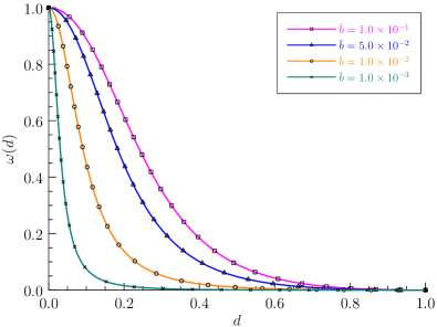
To be specific, let us discuss the Conti et al. (2016, 2024) model in more details. The degradation function (4.5) corresponds to the following cracking function

\displaystyle\phi(d)=\dfrac{1}{\bar{b}}\bigg{\langle}\dfrac{d^{2}}{(1-d)^{2}}-\bar{b}\bigg{\rangle}\qquad\Longrightarrow\qquad\bar{\phi}(d)=b\phi(d)=l_{\text{ch}}\bigg{\langle}\dfrac{d^{2}}{(1-d)^{2}}-\bar{b}\bigg{\rangle}

(4.7)

such that

\displaystyle\eta(d)=\dfrac{1}{l_{\text{ch}}}\dfrac{d^{2}\big{(}1-d\big{)}^{2}}{\big{\langle}d^{2}-\bar{b}\big{(}1-d\big{)}^{2}\big{\rangle}},\qquad\eta_{0}=\dfrac{1}{l_{\text{ch}}}\lim_{d\to 0}\dfrac{d^{2}}{\big{\langle}d^{2}-\bar{b}\big{\rangle}}=\begin{cases}+\infty&\qquad b\geq l_{\text{ch}}d^{2}\\ \dfrac{1}{l_{\text{ch}}}&\qquad b<l_{\text{ch}}d^{2}\\ \end{cases}

(4.8)

with the McAuley brackets $\langle x\rangle:=\max(0,x)$ .

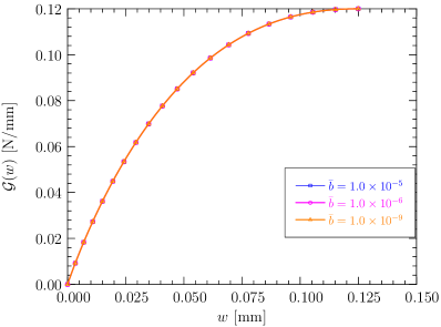
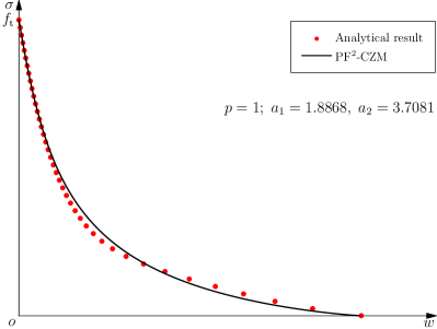
Upon the condition $\bar{b}<d^{2}$ , Eq. 3.2 gives the following TSL


$\displaystyle\sigma(d_{\ast})$	$\displaystyle=f_{\text{t}}\sqrt{l_{\text{ch}}\eta(d_{\ast})}$	(4.9a)
$\displaystyle\mathrm{\mathit{w}}(d_{\ast})$	$\displaystyle=\mathrm{\mathit{w}}_{\text{cL}}\sqrt{\eta(d_{\ast})}\int_{0}^{d_{\ast}}\sqrt{\dfrac{\bar{\phi}(\vartheta)/l_{\text{ch}}}{\eta(\vartheta)-\eta(d_{\ast})}}\;\text{d}\vartheta$	(4.9b)

Moreover, the surface energy density function (3.6) particularizes into

\displaystyle\mathcal{G}(d_{\ast})=2G_{\text{f}}\int_{0}^{d^{\ast}}\dfrac{\vartheta\sqrt{\eta(\vartheta)}}{\sqrt{\eta(\vartheta)-\eta(d_{\ast})}}\;\text{d}\vartheta

(4.10)

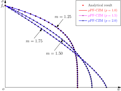
The above results are shown in Figure 1.

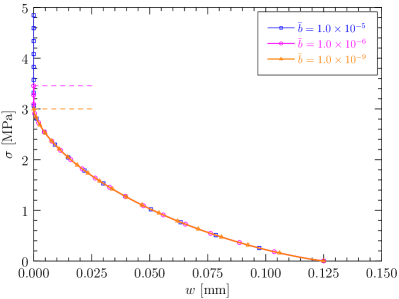
As can be seen, the value $\eta_{0}$ is well-defined (finite) and the nonlinear softening curve $\sigma(\mathrm{\mathit{w}})$ with a concave monotonically increasing surface energy density $\mathcal{G}(\mathrm{\mathit{w}})$ applies, if and only if $\bar{b}<d^{2}$ or, equivalently, $b<l_{\text{ch}}d^{2}$ . Consequently, the failure strength $f_{\text{t}}$ upon crack initiation is over-estimated for a finite value of the length scale parameter $b$ and is recovered only in the vanishing limit $b\to 0$ . In this sense, the Conti et al. (2016, 2024) model is length scale convergent.

Remark 4.1 Note that the following identity holds for the function $\bar{\phi}(d)$ given in Eq. 4.7₂

\displaystyle\lim_{b\to 0}\bar{\phi}(d)=l_{\text{ch}}\dfrac{d^{2}}{\big{(}1-d\big{)}^{2}}\qquad\Longrightarrow\qquad\lim_{b\to 0}\eta(d)=\dfrac{1}{l_{\text{ch}}}\big{(}1-d\big{)}^{2},\qquad\lim_{b\to 0}\eta_{0}=\dfrac{1}{l_{\text{ch}}}

(4.11)

That is, in the vanishing limit $b\to 0$ the truncation in the degradation function (4.5) is inactive. $\Box$

4.1.2 Limitations of the Conti et al. (2016, 2024) model

Though $\varGamma$ -convergence to the Barenblatt (1959) CZM has been proved, the Conti et al. (2016, 2024) model exhibits some practical limitations.

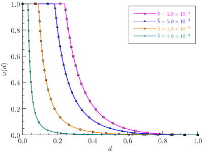
As shown in Figure 2(a), the degradation function (4.5) is truncated at the limit $\omega(d)=1$ and this truncation is activated except in the vanishing limit $b\to 0$ . Due to the presence of this truncation, the resulting energy functional is neither differentiable nor convex with respect to the crack phase-field. Moreover, the crack driving force vanishes when the truncation is activated, i.e., $\omega^{\prime}(d)=\varpi^{\prime}(d)=0$ .

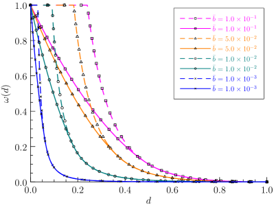
In order to address the above issues, Freddi and Iurlano (2017) suggested smoothening the truncated degradation function (4.5) by the following $\mathcal{C}^{1}$ -approximation

\displaystyle\omega(d)=\begin{cases}\Big{[}\hat{b}_{1}\big{(}d_{0}-d\big{)}+\hat{b}_{2}\Big{]}^{2}&\qquad 0\leq d\leq d_{0}\vspace{2mm}\\ \bar{b}\dfrac{\big{(}1-d\big{)}^{2}}{d^{2}}&\qquad d_{0}\leq d\leq 1\end{cases}

(4.12)

with the parameters

\displaystyle d_{0}=\dfrac{2\sqrt{\bar{b}}}{1+\sqrt{\bar{b}}},\qquad\hat{b}_{1}=\dfrac{\big{(}1+\sqrt{\bar{b}}\;\big{)}^{2}}{4\sqrt{\bar{b}}},\qquad\hat{b}_{2}=\dfrac{1-\sqrt{\bar{b}}}{2}

(4.13)

The above piece-wisely smoothened degradation function is depicted in Figure 2(b). As can be seen, the difference between these two functions vanishes for a vanishing limit $b\to 0$ . However, the smoothened degradation function (4.12) does not fulfill the necessary condition (4.3)

\displaystyle\lim_{d\to 0}d\cdot\bar{\omega}(d)=\dfrac{1}{\sqrt{b}}\cdot\lim_{d\to 0}d\cdot\Big{[}\hat{b}_{1}\big{(}d_{0}-d\big{)}+\hat{b}_{2}\Big{]}=0\notin(0,+\infty)

(4.14)

Moreover, it follows that

\displaystyle\eta_{0}=\dfrac{1}{l_{\text{ch}}}\lim_{d\to 0}\dfrac{1}{\bar{b}}\dfrac{d^{2}}{1-\big{[}\hat{b}_{1}\big{(}d_{0}-d\big{)}+\hat{b}_{2}\big{]}^{2}}=\dfrac{1}{l_{\text{ch}}}\lim_{d\to 0}\dfrac{d}{\bar{b}\hat{b}_{1}}=0\qquad\Longrightarrow\qquad\sigma_{\text{c}}=0

(4.15)

That is, crack nucleation occurs at the very beginning once the load is applied no matter how small it is. As a consequence, though the $\mathcal{C}^{1}$ -approximation (4.12) restores the differentiability and convexity of the total energy potential with respect to the crack phase-field, the issue of crack nucleation still presents.

4.2 Phase-field cohesive zone model (PF-CZM)

The aforesaid issues due to truncation in the degradation function (4.5) are overcome by the PF-CZM (Wu, 2018a; Wu and Nguyen, 2018). To this end, we present in this section a particular version of the PF-CZM corresponding to the Conti et al. (2016, 2024) model.

Noticing the identity (4.11), let us consider the following characteristic function $\bar{\phi}(d)$

\displaystyle\bar{\phi}(d)=l_{\text{ch}}\dfrac{d^{2}}{\big{(}1-d\big{)}^{2}}\qquad\Longrightarrow\qquad\eta(d)=\dfrac{1}{l_{\text{ch}}}\big{(}1-d\big{)}^{2},\qquad\eta_{0}=\dfrac{1}{l_{\text{ch}}}

(4.16)

such that the failure strength $\sigma_{\text{c}}=f_{\text{t}}$ is reproduced independently of the length scale parameter $b$ .

Accordingly, the cracking and dissipation functions are given by

\displaystyle\phi(d)=a_{0}\dfrac{d^{2}}{\big{(}1-d\big{)}^{2}},\qquad\omega(d)=\dfrac{\big{(}1-d\big{)}^{2}}{\big{(}1-d\big{)}^{2}+a_{0}d^{2}}\qquad\text{with}\qquad a_{0}=\dfrac{1}{\bar{b}}=\dfrac{l_{\text{ch}}}{b}

(4.17)

which fulfills the following property

\displaystyle\lim_{b\to 0}\dfrac{\big{(}1-d\big{)}^{2}}{\big{(}1-d\big{)}^{2}+a_{0}d^{2}}=\lim_{b\to 0}\bar{b}\dfrac{\big{(}1-d\big{)}^{2}}{\bar{b}\big{(}1-d\big{)}^{2}+d^{2}}=\bar{b}\dfrac{\big{(}1-d\big{)}^{2}}{d^{2}}

(4.18)

in the vanishing limit $b\to 0$ .

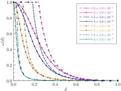
As shown in Figure 3, the degradation function (4.17) of rational fraction is a continuous approximation of the truncated one (4.5) adopted in the Conti et al. (2016, 2024) model, and both degradation functions coincide in the vanishing limit $b\to 0$ ; see Figure 1.

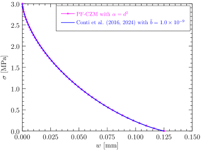
The parameterized TSL (3.2) can be expressed as the following closed-form


$\displaystyle\sigma(d_{\ast})$	$\displaystyle=f_{\text{t}}\big{(}1-d_{\ast}\big{)}$	(4.19a)
$\displaystyle\mathrm{\mathit{w}}(d_{\ast})$	$\displaystyle=\mathrm{\mathit{w}}_{\text{cL}}\Bigg{[}\arccos\big{(}1-d_{\ast}\big{)}-\big{(}1-d_{\ast}\big{)}\ln\dfrac{1+\sqrt{1-(1-d_{\ast})^{2}}}{1-d_{\ast}}\Bigg{]}$	(4.19b)

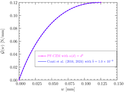
Moreover, the surface energy density function (3.6) is given by

\displaystyle\mathcal{G}(d_{\ast})=G_{\text{f}}\Bigg{[}\sqrt{1-(1-d_{\ast})^{2}}-\big{(}1-d_{\ast}\big{)}^{2}\ln\dfrac{1+\sqrt{1-(1-d_{\ast})^{2}}}{1-d_{\ast}}\Bigg{]}

(4.20)

which fulfills the properties (4.6) as expected. For the softening curve (4.19), the ultimate crack opening $\mathrm{\mathit{w}}_{\text{c}}$ and crack bandwidth $D(d_{\ast})$ are given by

\displaystyle\mathrm{\mathit{w}}_{\text{c}}:=\mathrm{\mathit{w}}(d_{\ast}=1)=\dfrac{\pi}{2}\mathrm{\mathit{w}}_{\text{cL}}=\dfrac{\pi G_{\text{f}}}{f_{\text{t}}},\qquad D(d_{\ast})=+\infty

(4.21)

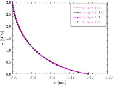
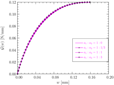
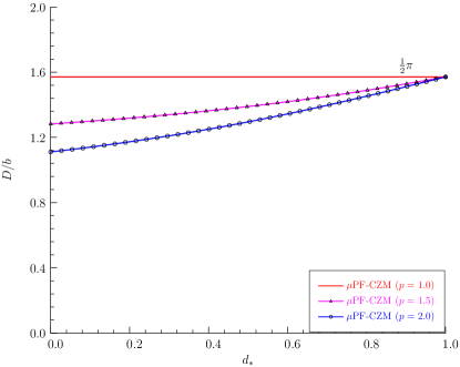
As the crack band is of infinite support once fracture is initiated, the condition (3.7) is automatically fulfilled. The above global responses, characterized by a particular nonlinear softening curve with a finite ultimate crack opening, are insensitive to the phase-field length scale parameter $b$ ; see Figure 4.

Remark 4.2 In the Conti et al. (2016, 2024) model and the PF-CZM counterpart, the degradation/dissipation function depends not only on the crack phase-field, but also on the length scale parameter. Though this dependence is introduced from different motivations, both models are closely inter-related and converges to the same CZM with a nonlinear softening curve in the vanishing limit $b\to 0$ . The difference is that the conditions (3.4) are fulfilled in the weak ( $\varGamma$ -convergent) sense for the Conti et al. (2016, 2024) model and in the strong (length scale insensitive) one for the PF-CZM, respectively.

5 Length scale insensitive phase-field cohesive zone model

In the Conti et al. (2016, 2024) model and the PF-CZM counterpart analyzed in Section 4, the associated formulation is considered together with the quadratic geometric function (4.1). In this section, the PF-CZM is discussed in the general form, with the non-associated formulation incorporated.

5.1 General formulation

The simplest function $\mu(d)$ fulfilling the conditions (2.22) might be of the following rational fraction

\displaystyle\mu(d)=a_{0}\dfrac{Q(d)}{\big{(}1-d\big{)}^{2p}}\qquad\text{with}\qquad Q(0)=0

(5.1)

for the parameter $a_{0}>0$ and the exponent $p\geq 1$ . Noticing the conditions $\alpha(0)=Q(0)=0$ , a natural choice is

\displaystyle Q(d)=\alpha(d)P(d)\qquad\Longrightarrow\qquad\mu(d)=a_{0}\dfrac{\alpha(d)}{h(d)}\qquad\text{with}\qquad h(d)=\dfrac{\big{(}1-d\big{)}^{2p}}{P(d)}

(5.2)

with the function $P(d)$ satisfying the condition $P(0)=1$ .

It then follows that

\displaystyle\eta(d)=\dfrac{\alpha(d)}{b\mu(d)}=\dfrac{1}{ba_{0}}h(d),\qquad\eta_{0}=\lim_{d\to 0}\eta(d)=\dfrac{1}{ba_{0}}\lim_{d\to 0}h(d)=\dfrac{1}{ba_{0}}

(5.3)

Accordingly, the length scale insensitivity conditions (3.4) imply

\displaystyle\eta_{0}=\dfrac{1}{ba_{0}}=\dfrac{c_{\alpha}}{2l_{\text{ch}}}\qquad\Longrightarrow\qquad a_{0}=\dfrac{2}{c_{\alpha}}\dfrac{l_{\text{ch}}}{b}

(5.4)

As can be seen, the parameter $a_{0}$ and the resulting function $\mu(d)$ are both inversely proportional to the length scale $b$ . This fact intrinsically guarantees the length scale insensitivity of the PF-CZM.

With the above function $\mu(d)$ , the parameterized TSL (3.2) becomes


$\displaystyle\sigma(d_{\ast})$	$\displaystyle=f_{\text{t}}\sqrt{h(d_{\ast})}$	(5.5a)
$\displaystyle\mathrm{\mathit{w}}(d_{\ast})$	$\displaystyle=\mathrm{\mathit{w}}_{\text{cL}}\dfrac{2}{c_{\alpha}a_{0}}\sqrt{h(d_{\ast})}\int_{0}^{d_{\ast}}\dfrac{\phi(\vartheta)\sqrt{h(\vartheta)/\alpha(\vartheta)}}{\sqrt{h(\vartheta)-h(d_{\ast})}}\;\text{d}\vartheta$	(5.5b)

Once the functions $\alpha(d)$ and $\phi(d)$ are known, the softening curve $\sigma(\mathrm{\mathit{w}})$ can be evaluated.

Vice versa, for a given TSL $\sigma(\mathrm{\mathit{w}})$ is given, the cracking function $\phi(d)$ can be solved as (Polyanin and Manzhirov, 2008; Feng et al., 2021; Wu, 2024)

\displaystyle\phi(d)=\dfrac{c_{\alpha}a_{0}}{\pi}\sqrt{\dfrac{\alpha(d)}{h(d)}}\;\bar{\varXi}(d)\qquad\text{with}\qquad\bar{\varXi}(d)=\dfrac{\partial}{\partial d}\Bigg{(}\int_{0}^{d}-\frac{1}{2}\dfrac{\bar{\mathrm{\mathit{w}}}(\vartheta)h^{\prime}(\vartheta)/\!\!\sqrt{h(\vartheta)}}{\sqrt{h(\vartheta)-h(d_{\ast})}}\;\text{d}\vartheta\Bigg{)}

(5.6)

such that the crack opening (5.5b) becomes

\displaystyle\mathrm{\mathit{w}}(d_{\ast})=\mathrm{\mathit{w}}_{\text{cL}}\bar{\mathrm{\mathit{w}}}(d_{\ast})\qquad\text{with}\qquad\bar{\mathrm{\mathit{w}}}(d_{\ast})=\dfrac{1}{\pi}\sqrt{h(d_{\ast})}\int_{0}^{d_{\ast}}\dfrac{\bar{\varXi}(\vartheta)}{\sqrt{h(\vartheta)-h(d_{\ast})}}\;\text{d}\vartheta

(5.7)

for the normalized one $\bar{\mathrm{\mathit{w}}}(d_{\ast}):=\mathrm{\mathit{w}}(d_{\ast})/\mathrm{\mathit{w}}_{\text{cL}}$ . As expected, the solved cracking function $\phi(d)$ also fulfills the conditions (2.21) as the dissipation function $\mu(d)$ does.

As stressed in Section 3.2, the above results hold only when the crack band does not shrink during the failure process, i.e.,

\displaystyle\dfrac{\partial D}{\partial d_{\ast}}\geq 0\qquad\text{with}\qquad D(d_{\ast})=b\int_{0}^{d_{\ast}}\dfrac{\sqrt{h(\vartheta)/\alpha(\vartheta)}}{\sqrt{h(\vartheta)-h(d_{\ast})}}\;\text{d}\vartheta

(5.8)

If the closed-form of Eq. 5.8 is not available, the condition (3.10) can be considered, i.e.,

\displaystyle D_{0}=\dfrac{\pi b}{\sqrt{\big{[}2p+P^{\prime}(0)\big{]}\alpha^{\prime}(0)}}\leq D_{\text{u}}=b\int_{0}^{1}\dfrac{1}{\sqrt{\alpha(\vartheta)}}\;\text{d}\vartheta

(5.9)

As can be seen, larger values $p\geq 1$ , $P^{\prime}(0)$ and $\alpha^{\prime}(0)$ are favorable for satisfaction of the condition (5.9).

5.2 Phase-field cohesive zone models with parameterized degradation function

In this section, for the geometric function (2.20) the associated PF-CZM is addressed, i.e.,


	$\displaystyle\phi(d)=\mu(d)=a_{0}\dfrac{\alpha(d)}{\big{(}1-d\big{)}^{2p}}P(d)$	(5.10a)
For the function $P(d)$ , Wu (2017) suggested using the following parameterized polynomial

	$\displaystyle P(d)=1+a_{1}d+a_{2}d^{2}+\cdots$	(5.10b)

with $a_{1}$ , $a_{2},\cdots$ being the parameters to be calibrated.

In this case, the crack opening $\mathrm{\mathit{w}}(d_{\ast})$ and surface energy density function $\mathcal{G}(d_{\ast})$ are evaluated as


$\displaystyle\mathrm{\mathit{w}}(d_{\ast})$	$\displaystyle=\mathrm{\mathit{w}}_{\text{cL}}\dfrac{2}{c_{\alpha}}\sqrt{h(d_{\ast})}\int_{0}^{d_{\ast}}\dfrac{\sqrt{\alpha(\vartheta)/h(\vartheta)}}{\sqrt{h(\vartheta)-h(d_{\ast})}}\;\text{d}\vartheta$	(5.11a)
$\displaystyle\mathcal{G}(d_{\ast})$	$\displaystyle=\dfrac{4G_{\text{f}}}{c_{\alpha}}\int_{0}^{d_{\ast}}\bigg{[}1-\dfrac{h(d_{\ast})}{h(\vartheta)}\bigg{]}^{-\frac{1}{2}}\sqrt{\alpha(\vartheta)}\;\text{d}\vartheta$	(5.11b)

For the geometric function (2.20) and the cracking function (5.10), it is rather difficult, if not impossible, to evaluate Eq. 5.11 analytically. Fortunately, the initial slope $k_{0}$ of the softening curve $\sigma(\mathrm{\mathit{w}})$ and the ultimate crack opening $\mathrm{\mathit{w}}_{\text{c}}$ can be determined in closed-form


$\displaystyle k_{0}:$	$\displaystyle=\lim_{d_{\ast}\to 0}\dfrac{\partial\sigma}{\partial\mathrm{\mathit{w}}}=\dfrac{c_{\alpha}}{2\pi\sqrt{\xi}}\big{(}2p+a_{1}\big{)}^{\frac{3}{2}}k_{\text{0L}}$	(5.12a)
$\displaystyle\mathrm{\mathit{w}}_{\text{c}}:$	$\displaystyle=\lim_{d_{\ast}\to 1}\mathrm{\mathit{w}}=\begin{cases}\dfrac{\pi}{c_{\alpha}}\mathrm{\mathit{w}}_{\text{cL}}\sqrt{P(1)}&\qquad p=1\\ +\infty&\qquad p>1\\ \end{cases}$	(5.12b)

for the initial slope $k_{\text{0L}}:=-\frac{1}{2}f_{\text{t}}^{2}/G_{\text{f}}$ of the linear softening law (A.1).

Accordingly, for a given TSL $\sigma(\mathrm{\mathit{w}})$ the parameters $a_{1}$ , $a_{2}$ ….., are determined as


		$\displaystyle a_{1}=\bigg{(}\dfrac{2\pi\sqrt{\xi}}{c_{\alpha}}\bar{k}_{0}\bigg{)}^{\frac{2}{3}}-2p$		(5.13a)
		$\displaystyle a_{2}+\cdots=\begin{cases}0&\qquad p>1\vspace{1mm}\\ \bigg{(}\dfrac{c_{\alpha}}{\pi}\bar{\mathrm{\mathit{w}}}_{\text{c}}\bigg{)}^{2}-\big{(}1+a_{1}\big{)}&\qquad p=1\\ \end{cases}$		(5.13b)

in terms of the ratios $\bar{k}_{0}:=k_{0}/k_{\text{0L}}$ and $\bar{\mathrm{\mathit{w}}}_{\text{c}}:=\mathrm{\mathit{w}}_{\text{c}}/\mathrm{\mathit{w}}_{\text{cL}}$ , respectively.

The above results apply upon the condition (5.9)

\displaystyle D_{0}=\dfrac{\pi b}{\sqrt{\xi\big{(}2p+a_{1}\big{)}}}=\pi b\bigg{(}\dfrac{2\pi\xi^{2}}{c_{\alpha}}\bar{k}_{0}\bigg{)}^{-\frac{1}{3}}\leq D_{\text{u}}\qquad\Longrightarrow\qquad\dfrac{2\pi\xi^{2}}{c_{\alpha}}\bar{k}_{0}\geq\bigg{(}\dfrac{\pi b}{D_{\text{u}}}\bigg{)}^{3}

(5.14)

For the polynomial geometric function (2.20), both the initial and ultimate crack bandwidths decrease monotonically with the parameter $\xi\in[0,2]$ , and the former decreases more rapidly (Wu, 2017). Dependent on the parameter $\xi\in[0,2]$ , the following PF-CZMs have been proposed in the literature:

\displaystyle\begin{cases}\text{PF${}^{\;0}$-CZM \cite[citep]{(\@@bibref{AuthorsPhrase1Year}{WZF2020}{\@@citephrase{, }}{})}}:&\xi=0,\;\alpha(d)=d^{2}\\ \text{PF${}^{\frac{1}{2}}$-CZM \cite[citep]{(\@@bibref{AuthorsPhrase1Year}{Wu2017,MBBPB2020}{\@@citephrase{, }}{})}}:&\xi=\frac{1}{2},\;\alpha(d)=\frac{1}{2}\big{(}d+d^{2}\big{)}\\ \text{PF${}^{\;1}$-CZM \cite[citep]{(\@@bibref{AuthorsPhrase1Year}{Lorentz2017,Wu2017,GLHTD2019}{\@@citephrase{, }}{})}}:&\xi=1,\;\;\alpha(d)=d\\ \text{PF${}^{\;2}$-CZM \cite[citep]{(\@@bibref{AuthorsPhrase1Year}{Wu2017,Wu2018,WN2018}{\@@citephrase{, }}{})}}:&\xi=2,\;\alpha(d)=2d-d^{2}\\ \end{cases}

In the following subsections some of them are discussed in more details.

5.2.1 PF⁰-CZM with the quadratic geometric function $\alpha(d)=d^{2}$

For brittle fracture the quadratic geometric function $\alpha(d)=d^{2}$ yields the popular AT2 model (Bourdin et al., 2000, 2008). It was also considered in the context of cohesive fracture (Wang et al., 2020)

\displaystyle\alpha(d)=d^{2}\qquad\Longrightarrow\qquad c_{\alpha}=2,\qquad a_{0}=\dfrac{l_{\text{ch}}}{b}

(5.15)

In this case, it follows from Eq. 5.12a that

\displaystyle\alpha^{\prime}(0)=\xi=0\qquad\Longrightarrow\qquad k_{0}=-\infty

(5.16)

As the initial slope $k_{0}$ is negatively infinite, Eq. 5.13a is indefinite. Therefore, in order to achieve a finite ultimate crack opening $\mathrm{\mathit{w}}_{\text{c}}$ , the exponent $p=1$ is considered, leading to

\displaystyle\mathrm{\mathit{w}}_{\text{c}}=\dfrac{\pi}{2}\mathrm{\mathit{w}}_{\text{cL}}\sqrt{P(1)}\qquad\Longrightarrow\qquad a_{1}+a_{2}+\cdots=\bigg{(}\dfrac{2}{\pi}\bar{\mathrm{\mathit{w}}}_{\text{c}}\bigg{)}^{2}-1

(5.17)

The PF-CZM presented in Section 4.2 is a particular instance with $a_{1}=a_{2}=\cdots=0$ , resulting in an ultimate crack opening $\mathrm{\mathit{w}}_{\text{c}}=\frac{1}{2}\pi\mathrm{\mathit{w}}_{\text{cL}}$ , i.e., $\bar{\mathrm{\mathit{w}}}_{\text{c}}=\frac{1}{2}\pi$ .

The softening curve and surface energy density function given by the above PF⁰-CZM are depicted in Figure 5. As can be seen, the PF⁰-CZM is characterized by a nonlinear softening curve $\sigma(\mathrm{\mathit{w}})$ and a surface energy density function $\mathcal{G}(\mathrm{\mathit{w}})$ approaching the Griffith (1921) fracture energy $G_{\text{f}}$ at the finite ultimate crack opening $\mathrm{\mathit{w}}=\mathrm{\mathit{w}}_{\text{c}}$ . Remarkably, the specific values of the parameters $a_{1}$ and $a_{2}$ have negligible effects on the results.

Remark 5.1 As in the AT2 model for brittle fracture, the crack bandwidth $D(d_{\ast})$ is infinite, i.e.,

\displaystyle D(d_{\ast})=+\infty

(5.18)

In this PF⁰-CZM, the crack phase-field needs to be solved in the whole domain. $\Box$

5.2.2 PF¹-CZM with the linear geometric function $\alpha(d)=d$

The geometric function $\alpha(d)=d$ or, equivalently, $\xi=1$ , has been adopted in the AT1 model for brittle fracture (Pham et al., 2011; Mesgarnejad et al., 2015) and in the Lorentz model for cohesive one (Lorentz, 2017; Geelen et al., 2019); see also Wu (2017).

In this case, it follows that

\displaystyle\alpha(d)=d\qquad\Longrightarrow\qquad c_{\alpha}=\dfrac{8}{3},\qquad a_{0}=\dfrac{3}{4}\dfrac{l_{\text{ch}}}{b},\qquad D_{\text{u}}=2b

(5.19)

The condition (5.14) for a non-shrinking crack band becomes

\displaystyle D_{0}=\dfrac{\pi b}{\sqrt{2p+a_{1}}}\leq D_{\text{u}}=2b\qquad\Longrightarrow\qquad 2p+a_{1}\geq\dfrac{1}{4}\pi^{2}\qquad\text{or}\qquad\bar{k}_{0}\geq\dfrac{\pi^{2}}{6}

(5.20)

That is, the PF¹-CZM applies only to those softening curves with the initial slope ratio $\bar{k}_{0}\geq\frac{1}{6}\pi^{2}$ .

To be more specific, let us consider the following two softening curves.

1.

Linear softening ( $\bar{k}_{0}=1$ ): For a finite ultimate crack opening, the exponent $p=1$ applies and Eq. 5.13 gives

$\displaystyle a_{1}=-0.2293,\qquad a_{2}=-0.0502\qquad\Longrightarrow\qquad D_{0}=2.36b\geq D_{\text{u}}=2b$ (5.21)

which violates the necessary condition (5.14). In other words, the PF¹-CZM should be used with cautions for linear softening.
2.

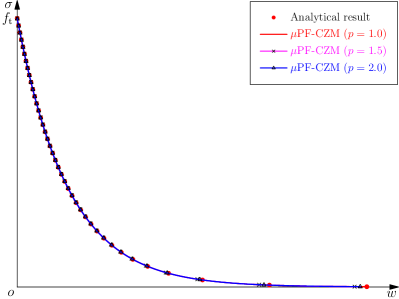
Exponential softening ( $\bar{k}_{0}=2$ ): For this softening curve with an infinite ultimate crack opening, the exponent $p=1.25>1$ applies and it then follows from Eq. 5.13 that

$\displaystyle a_{1}=0.3108,\qquad a_{2}=\cdots=0\qquad\Longrightarrow\qquad D_{0}=1.874b<D_{\text{u}}=2b$ (5.22)

As expected, for cohesive fracture with exponential softening the crack band is non-shrinking during the failure process and the PF¹-CZM applies.

5.2.3 PF²-CZM with the optimal geometric function $\alpha(d)=2d-d^{2}$

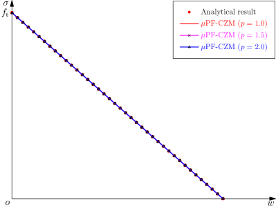
For cohesive fracture in brittle and quasi-brittle solids the most frequently adopted softening curves are either convex $\bar{k}_{0}>1$ or linear $\bar{k}_{0}=1$ . Let us consider the least favorable case of linear softening with $\bar{k}_{0}=1$ , the condition (5.14) becomes

\displaystyle\dfrac{2\pi\xi^{2}}{c_{\alpha}}\geq\bigg{(}\dfrac{\pi b}{D_{\text{u}}}\bigg{)}^{3}\qquad\Longrightarrow\qquad\xi=2,\qquad\alpha(d)=2d-d^{2},\qquad c_{\alpha}=\pi

(5.23)

That is, the geometric function $\alpha(d)=2d-d^{2}$ is optimal for the non-concave (linear and convex) softening curves with $\bar{k}_{0}\geq 1$ since the resulting PF²-CZM automatically guarantees a non-shrinking crack band (Wu, 2017).

Accordingly, the parameters $a_{1}$ , $a_{2}$ , $\cdots$ are determined as

\displaystyle a_{1}=2\big{(}\bar{k}_{0}^{\frac{2}{3}}-p\big{)},\qquad a_{2}+\cdots=\begin{cases}0&\qquad p>1\\ \bar{\mathrm{\mathit{w}}}_{\text{c}}^{2}-\big{(}1+a_{1}\big{)}&\qquad p=1\\ \end{cases}

(5.24)

For those commonly adopted non-concave softening curves, the following parameters apply

\displaystyle\begin{cases}p=1,\phantom{.35}\qquad a_{1}=a_{2}=\cdots=0&\qquad\text{Linear softening}\\ p=1.35,\qquad a_{1}=0.4748,\qquad a_{2}=\cdots=0&\qquad\text{Exponential softening}\\ p=1,\phantom{.35}\qquad a_{1}=1.8868,\qquad a_{2}=3.7081&\qquad\text{\cite[cite]{\@@bibref{Authors Phrase1YearPhrase2}{CHR1986}{\@@citephrase{(}}{\@@citephrase{)}}} softening}\\ \end{cases}

(5.25)

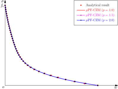
Figure 6 compares the softening curves predicted by Eqs. 5.5a and 5.11a against the target ones. Among them, the linear softening curve is exactly reproduced, while the discrepancies for the exponential one are invisible. For the Cornelissen et al. (1986) softening curve, the discrepancy is also acceptable and can be reduced by increasing the order of $P(d)$ as in Wu et al. (2023). Other non-concave softening curves can also be considered. Importantly, the crack bandwidth $D(d_{\ast})$ monotonically increases to a finite value $D_{u}=\frac{1}{2}\pi b$ for any non-concave softening curve.

5.3 Phase-field cohesive zone models with solved degradation function

In the PF-CZMs discussed in Section 5.2, the associated formulation is adopted and the degradation/dissipation function of rational fraction is postulated a priori in terms of a parameterized polynomial function (5.10b). Though the PF²-CZM with the optimal geometric function applies to linear and general convex softening behavior, those concave softening curves, e.g., the Park et al. (2009) one for adhesive fracture, cannot be considered. Aiming to address the above issues, the author (Wu, 2024) recently proposed the generalized phase-field cohesive zone model ( $\mu$ PF-CZM) with different degradation and dissipation functions. Almost any arbitrary TSL softening law can be reproduced with the condition (5.9) for a non-shrinking crack band intrinsically fulfilled.

In the $\mu$ PF-CZM, the simplest polynomial $P(d)$ is considered in Eq. 5.2

\displaystyle P(d)=1\qquad\Longrightarrow\qquad Q(d)=\alpha(d),\qquad\mu(d)=a_{0}\dfrac{\alpha(d)}{h(d)},\qquad h(d)=\big{(}1-d\big{)}^{2p}

(5.26)

In this case, the cracking function $\phi(d)$ given in Eq. 5.6 simplifies into

\displaystyle\phi(d)=a_{0}p\dfrac{c_{\alpha}}{\pi}\dfrac{\sqrt{\alpha(d)}}{\big{(}1-d\big{)}^{p+1}}\varXi(d)\qquad\text{with}\qquad\;\varXi(d)=\big{(}1-d\big{)}\dfrac{\partial}{\partial d}\Bigg{[}\int_{0}^{d}\dfrac{\bar{\mathrm{\mathit{w}}}(\vartheta)\big{(}1-\vartheta\big{)}^{p-1}}{\sqrt{h(\vartheta)-h(d)}}\;\text{d}\vartheta\Bigg{]}

(5.27)

where the function $\varXi(d)$ depends on the specific softening curve to be adopted. For instance, the following expressions were derived in Wu (2024)

\displaystyle\varXi(d)=\begin{cases}s(d)&\qquad\text{Linear softening}\\ \dfrac{1}{2}\text{arctanh}\big{(}s(d)\big{)}&\qquad\text{Exponential softening}\\ \bar{c}_{1}s+\bar{c}_{3}s^{3}+\bar{c}_{5}s^{5}+\big{(}\bar{c}_{2}s_{1}^{2}+\bar{c}_{4}s_{1}^{4}+\bar{c}_{6}s_{1}^{6}\big{)}\;\text{arctanh}\big{(}s(d)\big{)}&\qquad\text{6th-order polynomial softening}\\ \end{cases}

(5.28)

for the functions

\displaystyle s(d)=\sqrt{1-h(d)}=\sqrt{1-(1-d)^{2p}},\qquad s_{1}(d)=\sqrt{h(d)}=(1-d)^{p}

(5.29)

where the coefficients $\bar{c}_{i}\;(i=1,2,\cdots,6)$ for the 6th-order polynomial fitting of the Cornelissen et al. (1986) and Park et al. (2009) softening curves are given in A.

Accordingly, the traction–separation softening law parameterized in Eqs. 5.5a and 5.7 becomes


$\displaystyle\sigma(d_{\ast})$	$\displaystyle=f_{\text{t}}\big{(}1-d_{\ast}\big{)}^{p}$	(5.30a)
$\displaystyle\mathrm{\mathit{w}}(d_{\ast})$	$\displaystyle=\mathrm{\mathit{w}}_{\text{cL}}\big{(}1-d_{\ast}\big{)}^{p}\dfrac{1}{\pi}\int_{0}^{d_{\ast}}\dfrac{2p\varXi(\vartheta)/(1-\vartheta)}{\sqrt{h(\vartheta)-h(d_{\ast})}}\;\text{d}\vartheta$	(5.30b)

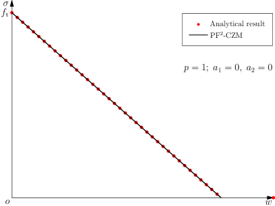
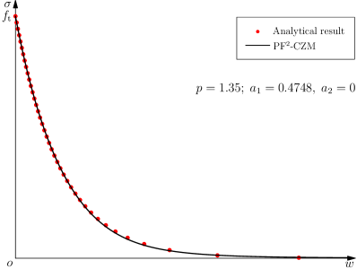
The resulting softening curve is depicted in Figure 7. As expected, all the linear, convex and concave softening curves can be reproduced independently of the exponent $p\geq 1$ (Wu, 2024).

Again, the above results holds upon the condition (3.7), with the crack bandwidth $D(d_{\ast})$ given by

\displaystyle\dfrac{\partial D}{\partial d_{\ast}}\geq 0\qquad\text{with}\qquad D(d_{\ast})=\int_{0}^{d_{\ast}}\dfrac{(1-\vartheta)^{p}}{\sqrt{\alpha(\vartheta)}}\cdot\dfrac{1}{\sqrt{h(\vartheta)-h(d_{\ast})}}\;\text{d}\vartheta

(5.31)

In particular, the condition (5.9) for a non-shrinking crack band becomes

\displaystyle D_{0}=\dfrac{\pi b}{\sqrt{2p\alpha^{\prime}(0)}}\leq D_{\text{u}}=b\int_{0}^{1}\dfrac{1}{\sqrt{\alpha(\vartheta)}}\;\text{d}\vartheta

(5.32)

from which the optimal geometric function $\alpha(d)$ can be determined.

Regarding whether the crack driving force is associated or non-associated, two strategies can be considered.

5.3.1 Associated formulation

Let us first discuss the associated formulation, i.e., $\phi(d)=\mu(d)$ . In this case, it follows from Eqs. 5.26 and 5.27 that

\displaystyle a_{0}\dfrac{\alpha(d)}{\big{(}1-d\big{)}^{2p}}=a_{0}p\dfrac{c_{\alpha}}{\pi}\dfrac{\sqrt{\alpha(d)}}{\big{(}1-d\big{)}^{p+1}}\;\varXi(d)\qquad\Longrightarrow\qquad\sqrt{\alpha(d)}=p\dfrac{c_{\alpha}}{\pi}\big{(}1-d\big{)}^{p-1}\varXi(d)

(5.33)

or, equivalently,

\displaystyle\sqrt{\alpha(d)}=\big{(}1-d\big{)}^{p-1}\varXi(d),\qquad c_{\alpha}=4\int_{0}^{1}\sqrt{\alpha(\vartheta)}\;\text{d}\vartheta=\dfrac{1}{p}\pi

(5.34)

Accordingly, the cracking function $\phi(d)$ is determined as

\displaystyle\phi(d)=\mu(d)=a_{0}\dfrac{\varXi^{2}(d)}{\big{(}1-d\big{)}^{2}}\qquad\text{with}\qquad a_{0}=\dfrac{2p}{\pi}\dfrac{l_{\text{ch}}}{b}

(5.35)

The TSL is still given by Eq. 5.30, with the following surface energy density function $\mathcal{G}(d_{\ast})$

\displaystyle\mathcal{G}(d_{\ast})=\dfrac{4p}{\pi}G_{\text{f}}\int_{0}^{d^{\ast}}\dfrac{\big{(}1-\vartheta\big{)}^{2p-1}\varXi(\vartheta)}{\sqrt{h(\vartheta)-h(d_{\ast})}}\;\text{d}\vartheta

(5.36)

Again, the above results hold provided the crack bandwidth $D(d_{\ast})$

\displaystyle D(d_{\ast})=b\int_{0}^{d_{\ast}}\dfrac{1-\vartheta}{\varXi(\vartheta)}\cdot\dfrac{1}{\sqrt{h(\vartheta)-h(d_{\ast})}}\;\text{d}\vartheta

(5.37)

is monotonically non-decreasing. Note that the lowest-order case of linear traction (i.e., $p=1$ ) recovers the particular version of the PF-CZM developed in Feng et al. (2021).

The associated $\mu$ PF-CZM has the merit that all the geometric and degradation/dissipation functions can be analytically determined in closed-form. However, the geometric function (5.34) is not optimal since the condition (5.32) cannot be a priori fulfilled. In order for better clarification, the following two particular softening curves are discussed.

Linear softening. For the parameterized traction (5.30a), linear softening gives

\displaystyle\bar{\mathrm{\mathit{w}}}(d_{\ast})=1-\big{(}1-d_{\ast}\big{)}^{p},\qquad\mathcal{G}(\mathrm{\mathit{w}}(d_{\ast}))=G_{\text{f}}\Big{[}1-\big{(}1-d_{\ast}\big{)}^{2p}\Big{]}=G_{\text{f}}\bar{\mathrm{\mathit{w}}}\big{(}2-\bar{\mathrm{\mathit{w}}}\big{)}

(5.38)

As shown in Figure 8(a), the surface energy density function $\mathcal{G}(\mathrm{\mathit{w}})$ approaches the fracture energy $G_{\text{f}}$ at the ultimate crack opening $\mathrm{\mathit{w}}=\mathrm{\mathit{w}}_{\text{cL}}$ (i.e., $\bar{\mathrm{\mathit{w}}}=1$ ) ⁴⁴4In Chen and de Borst (2021) only the first term in the energy dissipation (2.12) was accounted for, leading to the conclusion “the phase field method can partially produce the response of cohesive zone model, including the traction-separation law, but not entirely reproduce the cohesive response, which for instance holds for the dissipated energy.” However, with the missed second term in Eq. 2.12 was accounted for, the PF-CZM and $\mu$ PF-CZM can reproduce not only the TSL but also the energy dissipation, so long as the condition (5.31) is fulfilled..

Figure 8(b) presents evolution of the crack bandwidth (5.37) for various value of the traction order parameter $p\geq 1$ . As expected, the condition (5.32) is fulfilled for linear softening.

Exponential softening. For the parameterized traction (5.30a), exponential softening gives

\displaystyle\bar{\mathrm{\mathit{w}}}(d_{\ast})=-\dfrac{1}{2}\ln\big{(}1-d_{\ast}\big{)}^{p},\qquad\mathcal{G}(\mathrm{\mathit{w}}(d_{\ast}))=G_{\text{f}}\Big{[}1-\big{(}1-d_{\ast}\big{)}^{p}\Big{]}=G_{\text{f}}\Big{[}1-\exp\big{(}-2\bar{\mathrm{\mathit{w}}}\big{)}\Big{]}

(5.39)

As shown in Figure 9(a), the surface energy density function increases asymptotically to the fracture energy $G_{\text{f}}$ .

However, as shown in Figure 9(b), the increasing monotonicity of the crack bandwidth $D(d_{\ast})$ can only be guaranteed for the traction order parameter $p\geq 1.5$ . That is, for the traction order parameter $p<1.5$ , the crack band shrinks as cracking proceeds and some regions experience unloading. In such cases the crack irreversibility condition will affect the softening curve and the expected exponential one cannot be reproduced. This conclusion also applies to the Cornelissen et al. (1986) softening; see Wu (2024).

In summary, the associated $\mu$ PF-CZM with solved geometric function cannot always guarantee a non-shrinking crack band during the failure process and should be used with cautions.

Remark 5.2 Except for the case $p=1$ , the geometric function (5.34) vanishes both at $d=0$ and $d=1$ such that the increasing monotonicity (2.19)₂ is not satisfied. As a consequence, the associated $\mu$ PF-CZM with a higher-order exponent $p>1$ does not yield the expected crack profile of the bullet shape (Wu, 2024), though it is beneficial for guaranteeing a non-shrinking crack band. $\Box$

5.3.2 Non-associated formulation

The aforesaid issues exhibited by the associated $\mu$ PF-CZM were successfully removed in the recently proposed non-associated formulation (Wu, 2024). That is, the degradation function is different from the dissipation one, i.e., $\mu(d)\neq\phi(d)$ and $\varpi^{\prime}(d)\neq\omega^{\prime}(d)$ , though in some particular cases both functions may coincide.

In this case, as the geometric function $\alpha(d)$ does not affect the parameterized traction–separation law (5.30), an optimal expression can be determined from the condition (3.7) or (3.10). As proved in Wu (2024), regarding the parameterized polynomial function (2.20) with the parameter $\xi\in[0,2]$ , only the geometric function

\displaystyle\xi=2\qquad\Longrightarrow\qquad\alpha(d)=2d-d^{2},\qquad c_{\alpha}=\pi

(5.40)

is optimal for arbitrary softening curves and any traction order $p\geq 1$ in the sense that the resulting crack band is non-shrinking as expected; see Figure 10.

Correspondingly, the auxiliary dissipation function (5.26) and cracking function (5.27) become

\displaystyle\mu(d)=a_{0}\dfrac{2d-d^{2}}{\big{(}1-d\big{)}^{2p}},\qquad\phi(d)=a_{0}p\dfrac{\sqrt{2d-d^{2}}}{\big{(}1-d\big{)}^{p+1}}\cdot\varXi(d),\qquad a_{0}=\dfrac{2}{\pi}\dfrac{l_{\text{ch}}}{b}

(5.41)

In particular, for the linear softening curve and the lowest traction order $p=1$ , it follows that

\displaystyle\varXi(d)=\sqrt{2d-d^{2}}\qquad\Longrightarrow\qquad\phi(d)=\mu(d)=a_{0}\dfrac{2d-d^{2}}{\big{(}1-d\big{)}^{2}}

(5.42)

which is exactly the result of the PF²-CZM (Wu, 2017, 2018a; Wu and Nguyen, 2018) for linear softening.

Remark 5.3 Though the traction order parameter $p\geq 1$ does not affect the TSL $\sigma(\mathrm{\mathit{w}})$ , it does affect the crack bandwidth $D(d_{\ast})$ as shown in Figure 10. However, for various exponents $p\geq 1$ the ultimate crack bandwidths $D_{\text{u}}$ coincide since it depends only on the geometric function $\alpha(d)$ . $\Box$

6 Numerical examples

In Wu (2024), the non-associated $\mu$ PF-CZM was applied to the modeling of mode-I fracture in brittle and quasi-brittle solids. It was proved that the non-associated $\mu$ PF-CZM is sensitive neither to the phase-field length scale parameters as the original associated PF²-CZM nor to the traction order parameter $p\geq 1$ .

In this section, the non-associated $\mu$ PF-CZM is further validated against several numerical examples of concrete under mode-I and mixed-mode failure. For the sake of comparison, the numerical results predicted by the PF²-CZM are also presented. The Cornelissen et al. (1986) softening law is adopted for concrete. Note the minor difference of the softening curves given in Figure 6(c) by the PF²-CZM and in Figure 7(c) by the non-associated $\mu$ PF-CZM, respectively. Moreover, an extra example, which involves mode-I fracture with the concave Park et al. (2009) softening curve and thus defies the associated PF-CZM, is presented.

The numerical simulations were performed by our in-house code feFrac based on the open-source library jive (Nguyen-Thanh et al., 2020). Unstructured quadrilateral 4-node bilinear elements (Q4) generated by Gmsh (Geuzaine and Remacle, 2009) were used. Visualization was performed in Paraview (Ayachit, 2015).

6.1 Koyna dam under overflow pressure

The first example is mode-I fracture in the well-known Koyna dam under overflow pressure. As depicted in Figure 11, it is a concrete gravity dam of height 103 m. The initial crack length is 1.93 m, $10\%$ of the dam width at the location with varying slopes on the downstream face.

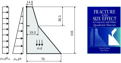
In the numerical simulation, the following material properties were adopted: Young’s modulus $E_{0}=2.5\times 10^{4}$ MPa, Poisson’s ratio $\nu_{0}=0.20$ , the failure strength $f_{\text{t}}=1.0$ MPa, the fracture energy $G_{\text{f}}=100$ J/m² and the mass density $\rho=2450$ kg/m³. The Rankine failure criterion (2.18)₁ was considered for mode-I fracture. The length scale parameter $b=0.3$ m and the mesh size $h_{e}=0.06$ m around the fracture process zone (FPZ) were considered. The loads were applied in three steps: in the first and second steps, the load control was used for the self weight and the full reservoir hydrostatic force, while in the third one for the overflow load with an increasing height, the indirect displacement control (Wu, 2018b) based on the horizontal displacement of the dam crest was employed. The simulations were run up to a horizontal displacement of 70 mm with an incremental size 0.5 mm.

As shown in Figure 12, the crack patterns predicted by the associated PF²-CZM and the non-associated $\mu$ PF-CZM with various values $p\geq 1$ almost coincide, and are fairly close to that printed on the book cover of the monograph (Bažant and Planas, 1997). In the early stage, a single crack initiates at the tip of the initial notch and extends downward to the downstream face. As the self-weight induced compressive stresses increases, the rate of crack propagation slows, leading to the occurrence of crack branching. A secondary crack then develops towards the intersecting point where the slope of the downstream face changes. The elevated compressive stresses in this region facilitate further crack branching.

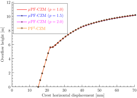
The responses of the dam, illustrated by the curve of overflow height versus crest horizontal displacement, are presented in Figure 13. As anticipated, the numerical results obtained from both the associated PF²-CZM and the non-associated $\mu$ PF-CZM with varying values of the traction order parameter $p\geq 1$ almost coincide. Notably, for overflow heights below approximately 5.5 m, fracture propagation is minimal, and the dam behaves in a nearly linear elastic manner. Following this, crack propagation occurs rapidly, leading to an initial decrease in the overflow level. A local maximum is observed in the overflow height versus displacement curve appears during the early stage, after which the relationship between crest displacement and overflow height becomes nonlinear.

6.2 Single edge-notched beam under proportional loading

The second example involves a single-edge notched beam (SENB) subjected to mixed-mode failure (Schlangen, 1993). As depicted in Figure 14, the beam has dimensions of 440 mm $\times$ 100 mm $\times$ 100 mm, with a notch of sizes 5 mm $\times$ 20 mm $\times$ 100 mm located at the top center. Two eccentrically proportional upward forces $10F^{\ast}/11$ and $F^{\ast}/11$ were exerted onto the two steel caps at the bottom of the beam. The relative vertical displacements on both sides of the notch, referred to as crack mouth sliding displacement (CMSD), was monitored to control the loading procedure. It was observed that a curved crack propagates from the notch downwards to the right hand side of the middle steel cap where the larger load was applied.

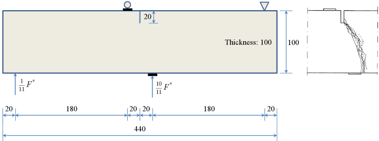
In the numerical simulation, the following mechanical parameters for concrete were adopted: Young’s modulus $E_{0}=3.2\times 10^{4}$ MPa, Poisson’s ratio $\nu_{0}=0.2$ , the failure strength $f_{\text{t}}=3.0$ MPa and the fracture energy $G_{\text{f}}=0.1$ N/mm. The modified von Mises failure criterion (2.18)₂ with the strength ratio $\rho_{s}=10.0$ was used in the modeling of mixed-mode failure. The phase-field length scale $b=1.0$ mm and the mesh size $h_{e}=0.2$ mm around the FPZ were considered. The simulation was performed using the CMSD based indirect displacement control (Wu, 2018b), with an incremental size 0.001 mm.

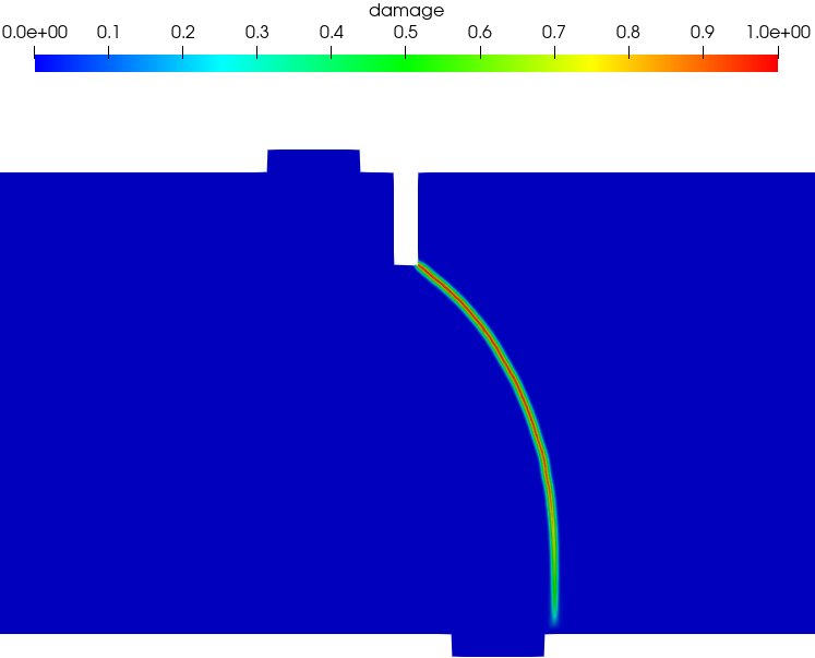
Figure 15 presents the predicted crack paths at the CMSD = 0.1 mm. As can be seen, the experimentally observed curved crack paths, propagating from the notch tip downward to the right hand side of the middle steel cap, were well captured by both the $\mu$ PF-CZM and PF²-CZM. Again, regarding the $\mu$ PF-CZM the traction order parameter $p\geq 1$ does not affect the crack path, though the crack tip is a bit more sharp for a larger value $p\geq 1$ .

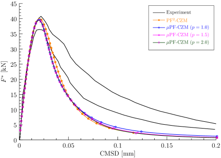
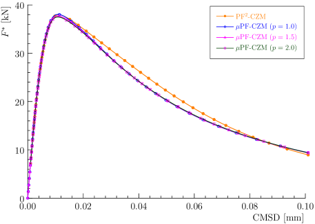
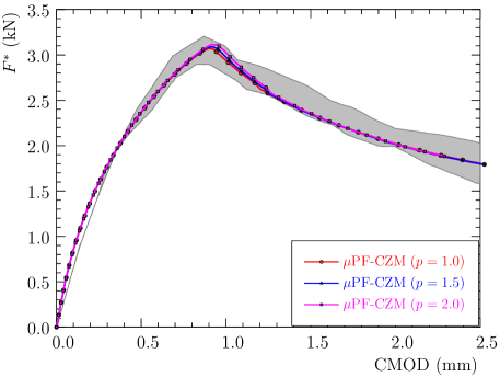
The numerical force versus CMSD curves are compared in Figure 16 against the test data. As can be seen, the discrepancy between the numerical results given by the non-associated $\mu$ PF-CZM and the associated PF²-CZM is minor. The predicted peak load agrees well with the test results and the overall agreement of the post-peak regime is also satisfactory. Moreover, the value of $p\geq 1$ has negligible effects on the global responses, verifying that the non-associated $\mu$ PF-CZM is indeed insensitive to the traction order parameter.

6.3 Double edge-notched beam under proportional loading

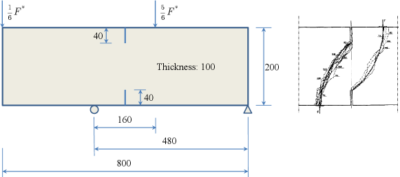
The next example is the four-point shear test of double edge-notched beams (DENB) reported in Bocca et al. (1990). As shown in Figure 17, the specimen was of dimensions 800 mm $\times$ 200 mm $\times$ 100 mm, with two notches of identical sizes 5 mm $\times$ 40 mm $\times$ 100 mm. Two eccentrically proportional downward forces $5F^{\ast}/6$ and $F^{\ast}/6$ were applied at the top of the beam. The CMSD of the notch was monitored to control the loading procedure.

In the numerical simulation, the following mechanical parameters for concrete were adopted: Young’s modulus $E_{0}=2.7\times 10^{4}$ MPa, Poisson’s ratio $\nu_{0}=0.18$ , the failure strength $f_{\text{t}}=2.0$ MPa and the fracture energy $G_{\text{f}}=0.1$ N/mm. Again, the modified von Mises failure criterion (2.18)₂ with the strength ratio $\rho_{s}=10.0$ was employed. The phase-field length scale $b=2.0$ mm and the mesh size $h_{e}=0.4$ mm around the FPZ were adopted. The CMSD-based indirect displacement control with an incremental size 0.001 mm was employed to track the equilibrium path.

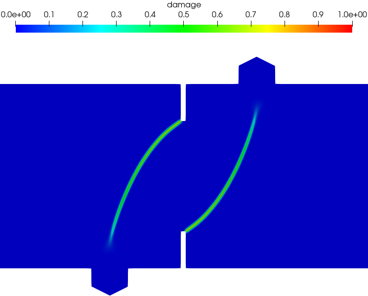
Figure 18 presents the numerically predicted crack paths at the CMSD = 0.1 mm. As can be seen, two anti-symmetric cracks initiate at the notch tips and propagate along curved paths to the two interior supports. Both the associated PF²-CZM and the non-associated $\mu$ PF-CZM are able to capture the mixed-mode failure with non-negligible shear stresses. Moreover, for the non-associated $\mu$ PF-CZM though the crack tip is a bit more sharp for a larger value of the traction order parameter $p\geq 1$ , the predicted crack pattern is unaffected.

The numerical load versus CMSD curves are depicted in Figure 19. As can be seen, the associated PF²-CZM and the non-associated $\mu$ PF-CZM give rather close predictions, though the post-peak softening behavior exhibits minor discrepancies due to the different approximations of the Cornelissen et al. (1986) softening curve. Again, the numerical results predicted by the non-associated $\mu$ PF-CZM are also insensitive to the traction order parameter $p\geq 1$ for this example involving mixed-mode failure.

6.4 Double edge-notched specimens under non-proportional loading

The test on the double edge-notched specimens (DENS) under non-proportional loading (Nooru-Mohamed, 1992) is another benchmark example of mixed fracture in concrete. As shown in Figure 20, the specimen was of dimensions 200 mm $\times$ 200 mm $\times$ 50 mm, with two identical notches of sizes 25 mm $\times$ 5 mm $\times$ 50 mm at the center of left and right edges. The specimen was glued to a rigid steel frame supported at the bottom and the right edge below the notch. In the test, a horizontal “shear” force $F_{s}^{\ast}$ was first imposed along the left edge above the notch, and then a vertical normal force $F^{\ast}$ was applied at the top edge with a monotonically increasing displacement $u^{\ast}$ while the shear force $F_{s}^{\ast}$ was maintained fixed. The specimens DENS-4a (48-03) and DENS-4b (46-05) were considered here, with the applied shear force $F_{s}^{\ast}$ being 5 kN and 10 kN, respectively. Experimental observation shows that two nearly antisymmetric cracks propagate from the notches to the opposite sides, with the curvature dependent on the level of the applied shear force $F_{s}^{\ast}$ .

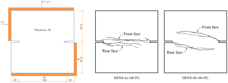
The following mechanical parameters for concrete were adopted in the numerical simulation: Young’s modulus $E_{0}=3.0\times 10^{4}$ MPa, Poisson’s ratio $\nu_{0}=0.2$ , the failure strength $f_{\text{t}}=3.0$ MPa and the fracture energy $G_{\text{f}}=0.11$ N/mm. As in the previous examples, the modified von Mises failure criterion (2.18)₂ with the strength ratio $\rho_{s}=10.0$ was used to model mixed-mode failure. The phase-field length scale $b=1.5$ mm and the mesh size $h=0.3$ mm around the FPZ were considered. Ths simulation was performed using the force control (20 and 40 equal increments for the DENS-4a and DENS-4b, respectively) for the shear stage and the displacement control with an incremental size 0.001 mm for the tensile stage.

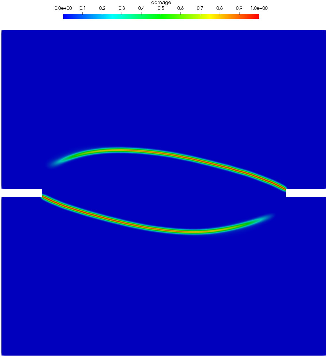
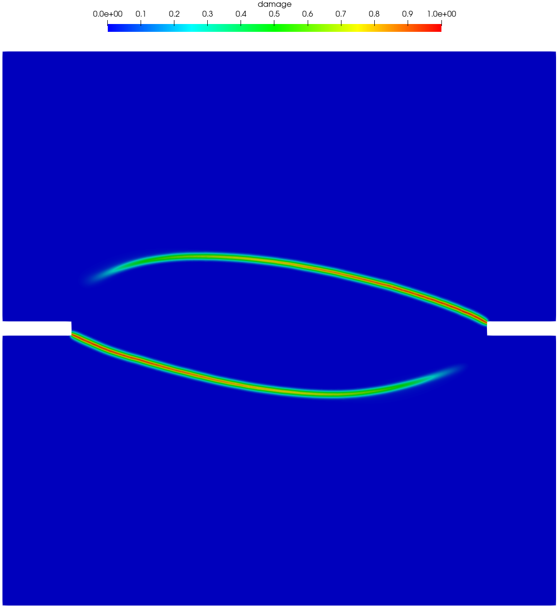
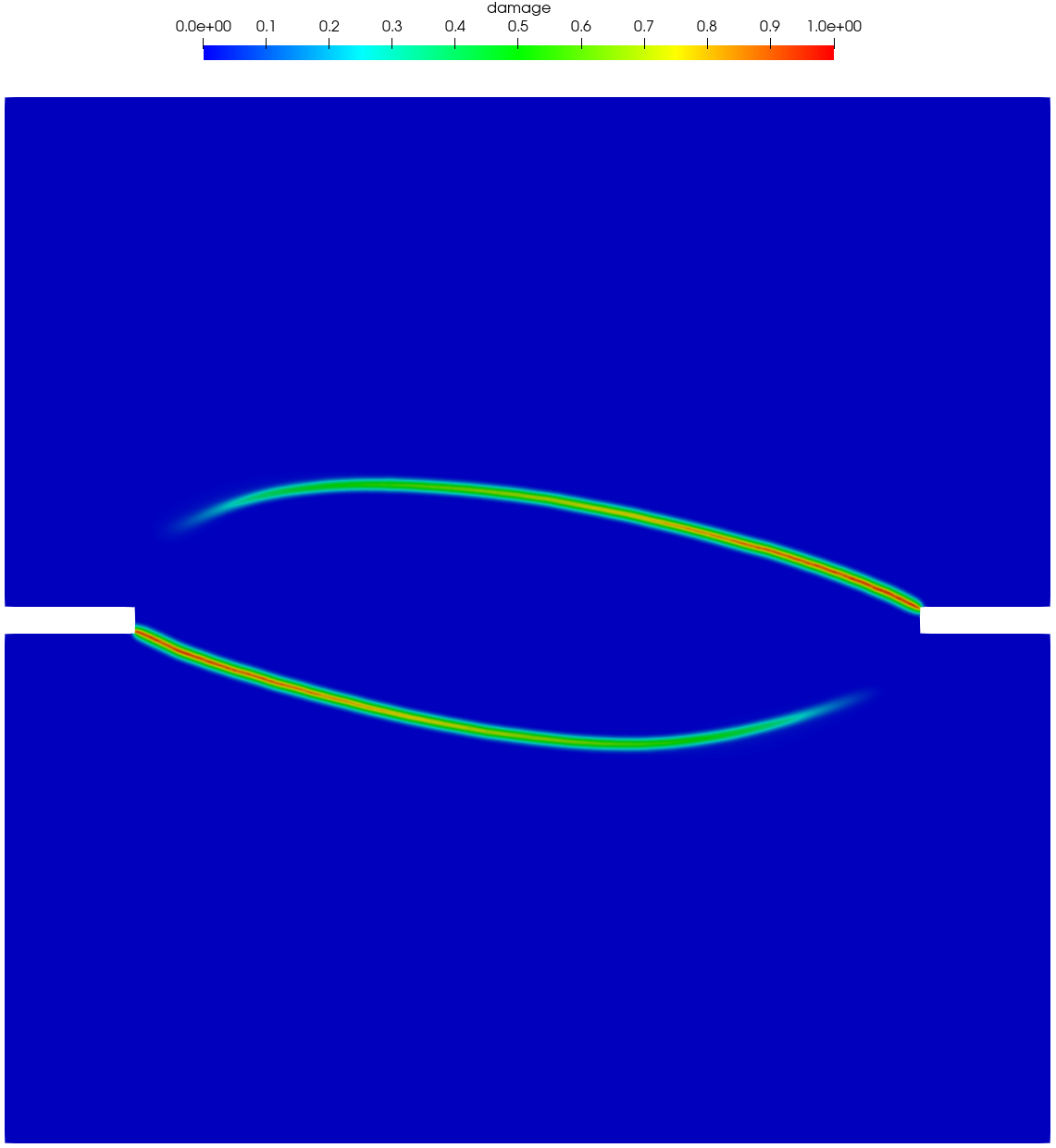
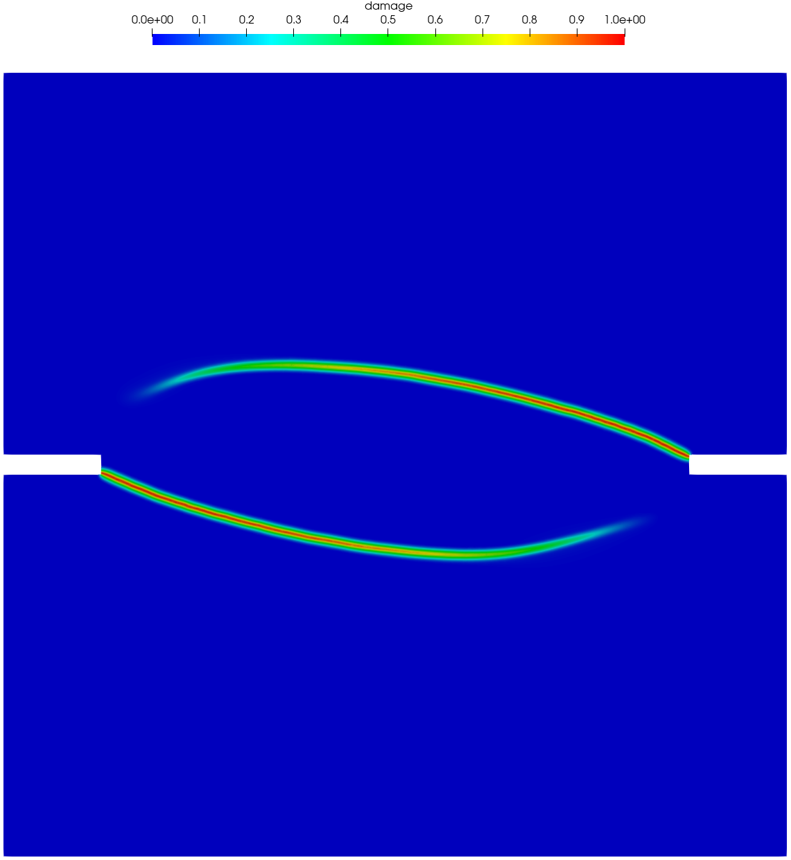
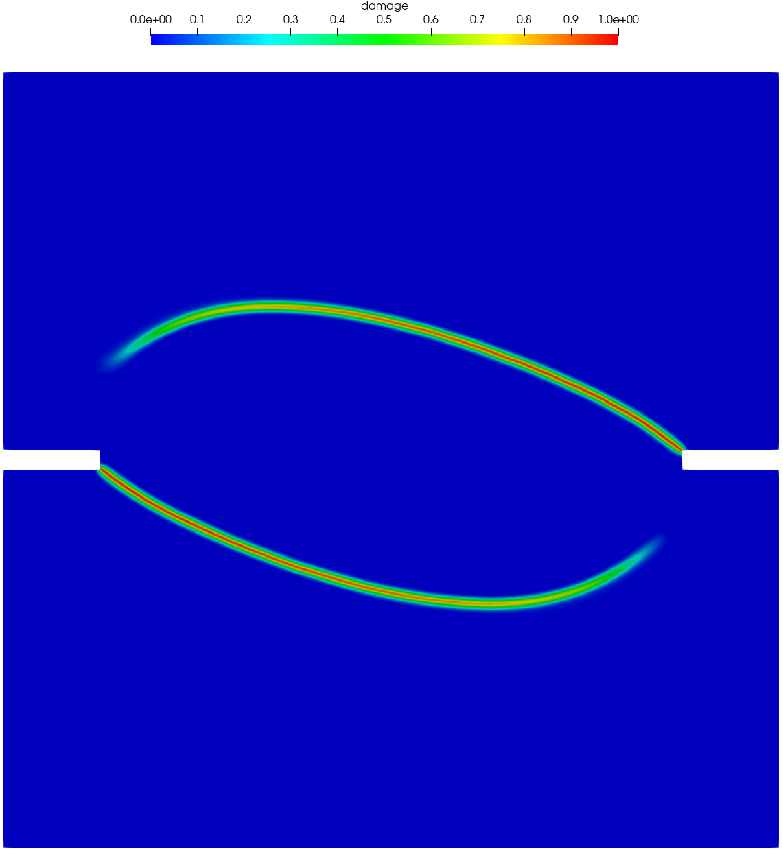
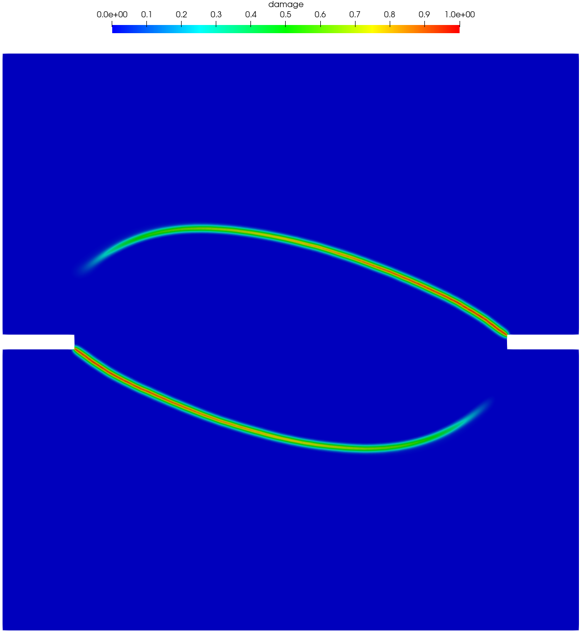
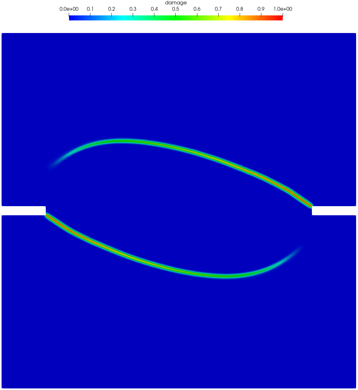
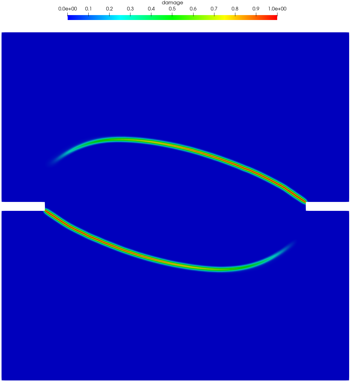
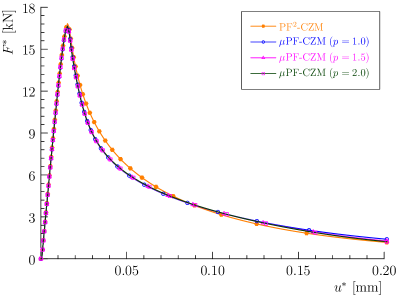
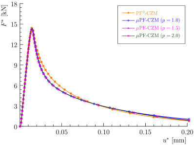
Figure 21 and Figure 22 present the numerically predicted crack patterns at the vertical displacement $u^{\ast}=0.2$ mm. As can be seen, all the numerical results agree qualitatively well with the experimentally observed crack paths — as the load level of the applied shear force $F_{s}^{\ast}$ increases, the curvature of the two anti-symmetric cracks becomes larger. Moreover, for the non-associated $\mu$ PF-CZM the traction order parameter $p\geq 1$ has negligible effects on the predicted crack pattern, though the crack tip is more sharp for a larger value $p$ .

The numerically predicted load versus displacement curves are depicted in Figure 23. As expected, the associated PF²-CZM and the non-associated $\mu$ PF-CZM give rather close numerical results. In particular, the vertical load capacity decreases as the load level of the applied shear force increases. Once the failure mechanism is fully developed, the vertical force tends to vanish completely and no stress locking is exhibited. Again, the traction order parameter $p\geq 1$ does not affect the global responses predicted by the non-associated $\mu$ PF-CZM.

6.5 Double cantilever beam test under mode-I failure

This final example involves the double cantilever beam (DCB) test reported in Alfano et al. (2009, 2010). The geometry, boundary and loading condition of the specimen is shown in Figure 24. Note that in Wu (2024), a similar but different specimen was considered and it was shown that the associated PF-CZM cannot be used for cohesive fracture with concave softening curves.

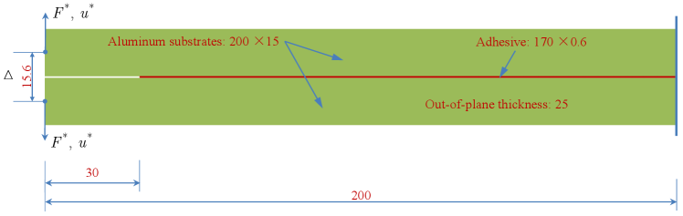
The specimen consists of two aluminum alloy (AA6060-TA16) substrates partially bonded with a toughened epoxy adhesive interface. The dimensions of each aluminum substrate are 200 mm $\times$ 15 mm $\times$ 25 mm, and those of the adhesive interface are 170 mm $\times$ 0.6 mm $\times$ 25 mm, respectively. The initial notch is 30 mm long measured from the left edge of the beams. Plane strain was assumed.

The aluminum substrates were considered using a linear elastic material with Young’s modulus 65.7 GPa and Poisson’s ratio 0.33. The adhesive layer was modeled by the non-associated $\mu$ PF-CZM with the following material parameters: Young’s modulus $E_{0}=1700$ MPa, Poisson’s ratio $\nu_{0}=0.35$ , the failure strength $f_{\text{t}}=10$ MPa and the fracture energy $G_{\text{f}}=4.0$ N/mm. The Rankine failure criterion (2.18)₁ and the Park et al. (2009) softening curve (A.8) with the exponent $m=1.15$ were adopted for the adhesive layer. The phase-field length scale parameter $b=0.1$ mm and the mesh size $h=0.02$ mm were considered in the numerical simulation.

(a)

p=1.0

(b)

p=1.5

(c)

p=2.0

(d) Zoomed crack profile around the notch

Figure 25: Double cantilever beam (DCB) test: Predicted crack profiles at CMOD = 2.5 mm.

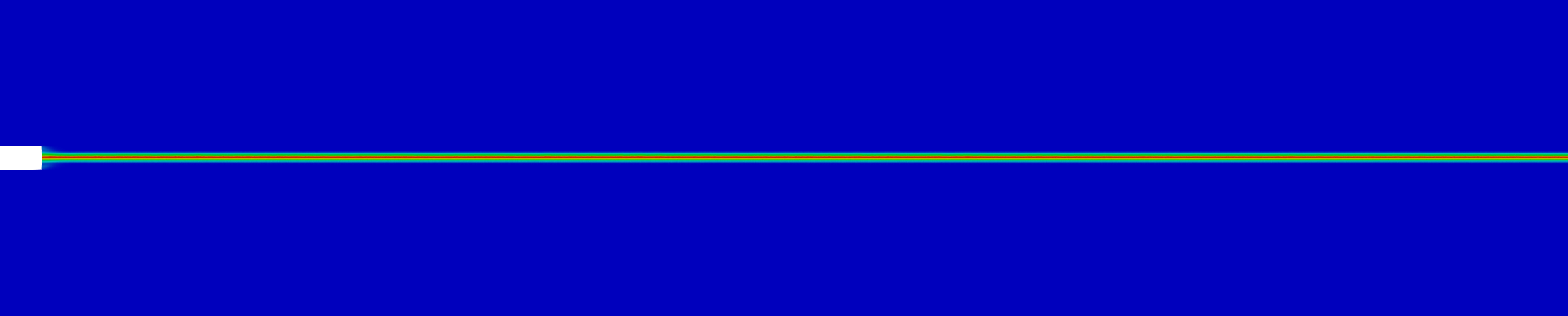
As shown in Figure 25, the crack propagates horizontally within the adhesive layer between two substrates. The traction order parameter $p\geq 1$ has negligible effects on the crack profile.

The numerical result of applied force versus CMOD curve is compared in Figure 26 against the experimental test data. As can be seen, the numerical results from various traction order parameters almost coincide and all agree well with the test data. The insensitivity to the traction order parameter is also validated for concave softening behavior.

7 Conclusions

In this work unified analysis of the existing phase-field models for cohesive fracture is addressed within the extended framework of the unified phase-field theory for fracture (Wu, 2017). Specifically, the Conti et al. (2016, 2024) model and the improved versions (Freddi and Iurlano, 2017; Lammen et al., 2023), the associated phase-field cohesive zone model (PF-CZM) (Wu, 2018a; Wu and Nguyen, 2018) and its variants (Lorentz, 2017; Wang, 2000; Feng et al., 2021), and the non-associated generalized phase-field cohesive zone model ( $\mu$ PF-CZM) (Wu, 2024) are systematically discussed. From the discussion the following conclusions can be drawn:

1.

All these models belong to the phase-field regularized counterpart of the Barenblatt (1959) cohesive zone model (CZM) by means of only the displacement field and the crack phase-field. They are distinguished by the characteristic functions involved in the formulation, i.e., the geometric function for the crack profile, the degradation function for the constitutive relation and the dissipation function for the crack driving force. The latter two characteristic functions coincide in the associated formulation, while in the non-associated one they are distinct. This distinction decouples the traction–separation softening law from the crack bandwidth, greatly facilitating the determination of the degradation function.
2.

In order for a phase-field model to be applicable to cohesive fracture, the length scale parameter has to be properly incorporated into the dissipation and/or degradation functions. Upon this incorporation, the resulting phase-field model converges to the Barenblatt (1959) CZM for a vanishing length scale parameter $b\to 0$ , with both the failure strength and the traction–separation softening curve being well-defined. Moreover, the resulting crack bandwidth needs to be non-decreasing during failure such that the target traction–separation softening law is recovered upon imposition of the crack irreversibility condition.
3.

The Conti et al. (2016, 2024) model, to the best knowledge of the author, might be the first phase-field model for cohesive fracture with the mathematical proof of $\varGamma$ -convergence available. With the degradation function being proportional to the length scale parameter, it converges in 1D case to the Barenblatt (1959) CZM with a particular nonlinear softening curve. However, due to the truncation in the degradation function, the resulting failure strength of finite value can only be achieved for a vanishing length scale $b\to 0$ . This deficiency not only limits its dealing with crack nucleation but also demands extremely fine mesh in the numerical simulation.
4.

The aforesaid issue of the Conti et al. (2016, 2024) model is removed by a particular version of the associated PF-CZM. Specifically, a continuous degradation/dissipation function of rational fraction, with its limit upon a vanishing length scale coincident with the one adopted in the Conti et al. (2016, 2024) model, is introduced. In this way, the truncation is no longer needed and the $\varGamma$ -convergence is preserved. Accordingly, the failure strength is independent of the incorporated length scale parameter and the traction–separation softening curve coincides with the limiting one of the Conti et al. (2016, 2024) model. The in-between correspondence justifies this particular version of the PF-CZM, though only a special softening curve can be considered.
5.

More general versions of the PF-CZM are discussed in a unified framework. With respect to the manner how the degradation function is determined, two groups of PF-CZMs are identified.

In the first group, only the associated formulation with identical degradation and dissipation functions is discussed. The dissipation/degradation function is assumed a priori to be of rational fraction characterized by a parameterized polynomial. The involved parameters are determined from the failure strength, the initial slope and the ultimate crack opening in closed-form. Moreover, it is found that the geometric function $\alpha(d)=2d-d^{2}$ is optimal in guaranteeing a non-shrinking crack band for the linear and general convex softening curves.

In the second group, the degradation function is solved analytically upon a simple relationship between the dissipation and geometric functions. Both the associated and non-associated formulations are considered. For the associated formulation, all the involved characteristic functions are determined in closed-form. Nevertheless, the so-determined geometric function cannot always guarantee the condition for a non-shrinking crack band, leading to the incapability of reproducing the anticipated traction–separation softening curve upon imposition of the crack irreversibility condition. Comparatively, for the non-associated formulation only the degradation function is solved analytically from the given softening curve independent of the geometric function. In this case the geometric function $\alpha(d)=2d-d^{2}$ is also optimal for any arbitrary softening curve and any traction order parameter $p\geq 1$ .
6.

Representative numerical examples indicate that the associated PF-CZM and the non-associated $\mu$ PF-CZM, both with the optimal geometric function, give rather close numerical predictions for cohesive fracture with linear and convex softening behavior. Not only the crack pattern but also the global response can be well captured by both models. However, the non-associated $\mu$ PF-CZM is advantageous since it applies to almost any arbitrary softening behavior including those concave ones. Moreover, it is insensitive not only to the phase-field length scale parameter, but also to the traction order exponent.

Currently the non-associated $\mu$ PF-CZM has been applied only to quasi-static problems. Its extension to fatigue scenario and to fracture in inelastic solids, among many others, can be considered in the forthcoming studies.

Acknowledgments

This work is supported by the National Natural Science Foundation of China (52125801) and Guangdong Provincial Key Laboratory of Modern Civil Engineering Technology (2021B1212040003) to the author (J.Y. Wu).

References

Alfano et al. (2009) Alfano, M., Furgiuele, F., Lenonardi, A., Maletta, C., Paulino, G., 2009. Mode-I fracture of adhesive joints using tailed cohesive zone models. International Journal of Fracture 157, 193–204.
Alfano et al. (2010) Alfano, M., Furgiuele, F., Pagnotta, L., Paulino, G.H., 2010. Analysis of fracture in aluminum joints bonded with a bi-componnet epoxy adhesive. Journal of Testing and Evaluation 39, JTE102753.
Ambati et al. (2015) Ambati, M., Gerasimov, T., de Lorenzis, L., 2015. A review on phase-field models for brittle fracture and a new fast hybrid formulation. Comput. Mech. 55, 383–405.
Ambrosio and Tortorelli (1990) Ambrosio, L., Tortorelli, V.M., 1990. Approximation of functional depending on jumps by elliptic functional via Gamma-convergence. Communications on Pure and Applied Mathematics 43, 999–1036.
Ayachit (2015) Ayachit, U., 2015. The ParaView guide: A parallel visualization application. Kitware, ISBN 978-1930934306.
Barenblatt (1959) Barenblatt, G.I., 1959. The formation of equilibrium cracks during brittle fracture. General ideas and hypotheses. Axially-symmetric cracks. Journal of Applied Mathematics and Mechanics 23, 622–636.
Bažant and Planas (1997) Bažant, Z.P., Planas, J., 1997. Fracture and size effects in concrete and other quasi-brittle materials. CRC Press, New York.
Bocca et al. (1990) Bocca, P., Carpinteri, A., Valente, S., 1990. Size effects in the mixed mode crack propagation: Softening and snap-back analysis. Engineering Fracture Mechanics 35, 159–170.
Bourdin et al. (2000) Bourdin, B., Francfort, G., Marigo, J.J., 2000. Numerical experiments in revisited brittle fracture. J. Mech. Phys. Solids 48, 797–826.
Bourdin et al. (2008) Bourdin, B., Francfort, G., Marigo, J.J., 2008. The variational approach to fracture. Springer, Berlin.
Braides (1998) Braides, A., 1998. Approximation of free-discontinuity problems. Springer science & Business Media, Berlin.
Chen and de Borst (2021) Chen, L., de Borst, R., 2021. Phase-field modeling of cohesive fracture. European Journal of Mechanics / A Solids 90, 104343.
Chen and de Borst (2022) Chen, L., de Borst, R., 2022. Phase-field regularised cohesive zone model for interface modelling. Theoretical and Applied Fracture Mechanics 122, 103630.
Conti et al. (2016) Conti, S., Focardi, M., Iurlano, F., 2016. Phase field approximation of cohesive fracture models. Annales de l’Institut Henri Poincare (C) Non Linear Analysis 33, 1033–1067.
Conti et al. (2024) Conti, S., Focardi, M., Iurlano, F., 2024. Phase-field approximation of a vectorial, geometrically nonlinear cohesive fracture energy. Arch. Rational Mech. Anal. 248, 21.
Cornelissen et al. (1986) Cornelissen, H., Hordijk, D., Reinhardt, H., 1986. Experimental determination of crack softening characteristics of normalweight and lightweight concrete. Heron 31, 45–56.
Feng et al. (2021) Feng, F., Fan, J., Li, J., 2021. Endowing explicit cohesive laws to the phase-field fracture theory. Journal of the Mechanics and Physics of Solids 152, 104464.
Francfort and Marigo (1998) Francfort, G., Marigo, J., 1998. Revisting brittle fracture as an energy minimization problem. J. Mech. Phys. Solids 46, 1319–1342.
Freddi and Iurlano (2017) Freddi, F., Iurlano, F., 2017. Numerical insight of a variational smeared approach to cohesive fracture. J. Mech. Phys. Solids 98, 156–171.
Geelen et al. (2019) Geelen, R.J.M., Liu, Y., Hu, T., Tupek, M.R., Dolbow, J.E., 2019. A phase-field formulation for dynamic cohesive fracture. Comput. Methods Appl. Mech. Eng. 34, 680–711.
Geuzaine and Remacle (2009) Geuzaine, C., Remacle, J.F., 2009. Gmsh: a three-dimensional finite element mesh generator with built-in pre- and post-processing facilities. Int. J. Numer. Engng 79(11), 1309–1331.
Griffith (1921) Griffith, A.A., 1921. The phenomena of rupture and flow in solids. Philosophical Transactions of the Royal Society of Londres 221, 163–198.
Kamarei et al. (2024) Kamarei, F., Kumar, A., Lopez-Pamies, O., 2024. The poker-chip experiments of synthetic elastomers explained. J. Mech. Phys. Solids 188, 105683.
Kumar et al. (2020) Kumar, A., Bourdin, B., Francfort, G.A., Lopez-Pamies, O., 2020. Revisiting nucleation in the phase-field approach to brittle fracture. Journal of the Mechanics and Physics of Solids 142, 104027.
Kupfer et al. (1969) Kupfer, H., Hilsdorf, H.K., Rusch, H., 1969. Behaviour of concrete under biaxial stress. Proc. ACI 66, 656–666.
Lammen et al. (2023) Lammen, H., Conti, S., Mosler, J., 2023. A finite deformation phase field model suitable for cohesive fracture. Journal of the Mechanics and Physics of Solids 178, 105349.
Larsen (2024) Larsen, C., 2024. A local variational principle for fracture. Journal of the Mechanics and Physics of Solids 187, 105625.
Larsen et al. (2024) Larsen, C., Dolbow, J., Lopez-Pamies, O., 2024. A variational formulation of griffith phase-field fracture with material strength. International Journal of Fracture doi: https://doi.org/10.1017/s10704-024-00786-3.
Lee et al. (2003) Lee, S.K., Song, Y.C., Han, S.H., 2003. Biaxial behavior of plain concrete of nuclear containment building. Nucl. Eng. Des. 227, 143–153.
Li and Guo (1991) Li, W.Z., Guo, Z.H., 1991. Experimental research for strength and deformation of concrete under biaxial tension–compression loading. J. Hydraul. Eng. (in Chinese) 8, 51–56.
Lorentz (2017) Lorentz, E., 2017. A nonlocal damage model for plain concrete consistent with cohesive fracture. Int. J. Fract. 207, 123–159.
Lorentz et al. (2012) Lorentz, E., Cuvilliez, S., Kazymyrenko, K., 2012. Modelling large crack propagation: from gradient-damage to cohesive zone models. Int. J. Fract. 178, 85–95.
Lorentz and Godard (2011) Lorentz, E., Godard, V., 2011. Gradient damage models: Towards full-scale computations. Comput. Methods Appl. Mech. Engrg. 200, 1927–1944.
Marboeuf et al. (2020) Marboeuf, A., Bennani, L., Budinger, M., Pommier-Budinger, V., 2020. Electromechanical resonant ice protection systems: numerical investigation through a phase-field mixed adhesive/brittle fracture model. Engineering Fracture Mechanics 230, 106926.
Mesgarnejad et al. (2015) Mesgarnejad, A., Bourdin, B., Khonsari, M., 2015. Validation simulations for the variational approach to fracture. Comput. Methods Appl. Mech. Engrg. 290, 420–437.
Miehe et al. (2010a) Miehe, C., Welschinger, F., Hofacker, M., 2010a. Thermodynamically consistent phase-field models of fracture: Variational principles and multi-field fe implementations. Int. J. Numer. Meth. Engng. 83, 1273–1311.
Mumford and Shah (1989) Mumford, D., Shah, J., 1989. Optimal approximations by piecewise smooth functions and associated variational problems. Communications on Pure and Applied Mathematics 42, 577–685.
Muneton-Lopez and Giraldo-Londono (2024) Muneton-Lopez, R.A., Giraldo-Londono, O., 2024. A phase-field formulation for cohesive fracture based on the park-paulino-roesler (PPR) cohesive fracture model. Journal of the Mechanics and Physics of Solids 182, 105460.
Nguyen et al. (2016) Nguyen, T.T., Yvonnet, J., Zhu, Q.Z., Bornert, M., Chateau, C., 2016. A phase-field method for computational modeling of interfacial damage interacting with crack propagation in realistic microstructures obtained by microtomography. Computer Methods in Applied Mechanics and Engineering 312, 567 – 595.
Nguyen-Thanh et al. (2020) Nguyen-Thanh, C., Nguyen, V.P., de Vaucorbeilc, A., Mandal, T.K., Wu, J.Y., 2020. Jive: an open source, research-oriented c++ library for solving partial differential equations. Advances in Engineering Software , 102925.
Nooru-Mohamed (1992) Nooru-Mohamed, M., 1992. Mixed-mode fracture of concrete: an experimental approach. Ph.D. thesis. Delft University of Technology.
Park et al. (2009) Park, K., Paulino, G., Roesler, J., 2009. A unified potential-based cohesive model for mixed-mode fracture. Journal of the Mechanics and Physics of Solids 57, 891–908.
Pham et al. (2011) Pham, K., Amor, H., Marigo, J.J., Maurini, C., 2011. Gradient damage models and their use to approximate brittle fracture. International Journal of Damage Mechanics 20, 618–652.
Polyanin and Manzhirov (2008) Polyanin, A., Manzhirov, A., 2008. Handbook of integral equations. CRC Press.
Schlangen (1993) Schlangen, E., 1993. Experimental and numerical analysis of fracture processes in concrete. Ph.D. thesis. Delft University of Technology.
Verhoosel and de Borst (2013) Verhoosel, C.V., de Borst, R., 2013. A phase-field model for cohesive fracture. Int. J. Numer. Meth. Engng. 96, 43–62.
Wang et al. (2020) Wang, Q., Zhou, W., Feng, Y.T., 2020. The phase-field model with an auto-calibrated degradation function based on general softening laws for cohesive fracture. Applied Mathematical Modelling 86, 185–206.
Wang (2000) Wang, T., 2000. Analysis of strip electric saturation model of crack problem in piezoelectric materials. International Journal of Solids and Structures 37, 6031–6049.
Wu (2017) Wu, J.Y., 2017. A unified phase-field theory for the mechanics of damage and quasi-brittle failure in solids. Journal of the Mechanics and Physics of Solids 103, 72–99.
Wu (2018a) Wu, J.Y., 2018a. A geometrically regularized gradient-damage model with energetic equivalence. Comput. Methods Appl. Mech. Engrg. 328, 612–637.
Wu (2018b) Wu, J.Y., 2018b. Robust numerical implementation of non-standard phase-field damage models for failure in solids. Computer Methods in Applied Mechanics and Engineering 340, 767–797.
Wu (2024) Wu, J.Y., 2024. A generalized phase-field cohesive zone model ( $\mu$ PF-CZM) for fracture. Journal of the Mechanics and Physics of Solids 192, 105841.
Wu and Cervera (2015) Wu, J.Y., Cervera, M., 2015. On the equivalence between traction- and stress-based approaches for the modeling of localized failure in solids. Journal of the Mechanics and Physics of Solids 82, 137–163.
Wu and Cervera (2016) Wu, J.Y., Cervera, M., 2016. A thermodynamically consistent plastic-damage framework for localized failure in quasi-brittle solids: Material model and strain localization analysis. International Journal of Solids and Structures 88-89, 227–247.
Wu et al. (2020a) Wu, J.Y., Huang, Y., Nguyen, V.P., 2020a. On the BFGS monolithic algorithm for the unified phase field damage theory. Comput. Methods Appl. Mech. Engrg. 360, 112704.
Wu and Nguyen (2018) Wu, J.Y., Nguyen, V.P., 2018. A length scale insensitive phase-field damage model for brittle fracture. Journal of the Mechanics and Physics of Solids 119, 20–42.
Wu et al. (2020b) Wu, J.Y., Nguyen, V.P., Nguyen, C.T., Sutula, D., Sinaie, S., Bordas, S., 2020b. Phase field modeling of fracture. Advances in Applied Mechancis 53, 1–183; https://doi.org/10.1016/bs.aams.2019.08.001.
Wu et al. (2023) Wu, J.Y., Yao, J.R., Le, J.L., 2023. Phase-field modeling of stochastic fracture in heterogeneous quasi-brittle solids. Comput. Methods Appl. Mech. Engrg. 416, 116332.
Zolesi and Maurini (2024) Zolesi, C., Maurini, C., 2024. Stability and crack nucleation in variational phase-field models of fracture: Effects of length-scales and stress multi-axiality. J. Mech. Phys. Solids 192, 105802.

Appendix A Softening curves

In this work, the following softening curves are considered.

Linear softening

\displaystyle\mathcal{G}(\mathrm{\mathit{w}})=\begin{cases}G_{\text{f}}\dfrac{\mathrm{\mathit{w}}}{\mathrm{\mathit{w}}_{\text{cL}}}\Big{(}2-\dfrac{\mathrm{\mathit{w}}}{\mathrm{\mathit{w}}_{\text{cL}}}\Big{)}&\qquad\text{if}\;\mathrm{\mathit{w}}\leq\mathrm{\mathit{w}}_{\text{cL}}\\ G_{\text{f}}&\qquad\text{if}\;\mathrm{\mathit{w}}\geq\mathrm{\mathit{w}}_{\text{cL}}\end{cases}\qquad\sigma(\mathrm{\mathit{w}})=f_{\text{t}}\max\Big{(}1-\dfrac{f_{\text{t}}}{2G_{\text{f}}}\mathrm{\mathit{w}},0\Big{)}

(A.1)

with the following initial slope $k_{0}$ and ultimate crack opening $\mathrm{\mathit{w}}_{\text{c}}$

\displaystyle k_{0}=k_{\text{0L}}=-\dfrac{f_{\text{t}}^{2}}{2G_{\text{f}}},\qquad\mathrm{\mathit{w}}_{\text{c}}=\mathrm{\mathit{w}}_{\text{cL}}=\dfrac{2G_{\text{f}}}{f_{\text{t}}}

(A.2)

Exponential softening

\displaystyle\mathcal{G}(\mathrm{\mathit{w}})=G_{\text{f}}\bigg{[}1-\exp\Big{(}-\dfrac{f_{\text{t}}}{G_{\text{f}}}\mathrm{\mathit{w}}\Big{)}\bigg{]},\qquad\sigma(\mathrm{\mathit{w}})=f_{\text{t}}\exp\Big{(}-\dfrac{f_{\text{t}}}{G_{\text{f}}}\mathrm{\mathit{w}}\Big{)}

(A.3)

with the following initial slope and ultimate crack opening

\displaystyle k_{0}=-\dfrac{f_{\text{t}}^{2}}{G_{\text{f}}},\qquad\mathrm{\mathit{w}}_{\text{c}}=+\infty

(A.4)

Cornelissen et al. (1986) softening

\displaystyle\sigma(\mathrm{\mathit{w}})=f_{\text{t}}\Big{[}\big{(}1.0+\eta_{1}^{3}r^{3}\big{)}\exp\big{(}-\eta_{2}r\big{)}-r\big{(}1.0+\eta_{1}^{3}\big{)}\exp\big{(}-\eta_{2}\big{)}\Big{]}\qquad\text{with}\qquad r:=\mathrm{\mathit{w}}/\mathrm{\mathit{w}}_{\text{c}}

(A.5)

for the initial slope $k_{0}$ and ultimate crack opening $\mathrm{\mathit{w}}_{\text{c}}$

\displaystyle k_{0}=-1.3546\dfrac{f_{\text{t}}^{2}}{G_{\text{f}}},\qquad\mathrm{\mathit{w}}_{\text{c}}=5.1361\dfrac{G_{\text{f}}}{f_{\text{t}}}

(A.6)

where the typical values $\eta_{1}=3.0$ and $\eta_{2}=6.93$ have been considered for normal concrete.

For the 6th-order polynomial fitting of this softening curve, the coefficients $\bar{c}_{n}$ in Eq. 5.28 are given by (Wu, 2024)


$\displaystyle\bar{c}_{1}$	$\displaystyle=\;101.6763,\quad\bar{c}_{2}=-40.4105,\quad\bar{c}_{3}=-129.1615$	(A.7a)
$\displaystyle\bar{c}_{4}$	$\displaystyle=-60.6300,\quad\bar{c}_{5}=\phantom{-}30.0532,\quad c_{6}=\;-0.2668$	(A.7b)

Park et al. (2009) softening

\displaystyle\mathcal{G}(\mathrm{\mathit{w}})=G_{\text{f}}\Bigg{[}1-\bigg{(}1-\dfrac{f_{\text{t}}}{mG_{\text{f}}}\mathrm{\mathit{w}}\bigg{)}^{m}\Bigg{]},\qquad\sigma(\mathrm{\mathit{w}})=f_{\text{t}}\Big{(}1-\dfrac{f_{\text{t}}}{mG_{\text{f}}}\mathrm{\mathit{w}}\Big{)}^{m-1}

(A.8)

with the initial slope $k_{0}$ and ultimate crack opening $\mathrm{\mathit{w}}_{\text{c}}$

\displaystyle k_{0}=-\dfrac{m-1}{m}\dfrac{f_{\text{t}}^{2}}{G_{\text{f}}},\qquad\mathrm{\mathit{w}}_{\text{c}}=m\dfrac{G_{\text{f}}}{f_{\text{t}}}

(A.9)

where the exponent $m>1$ controls the shape of the softening curve, i.e., convex for $m>2$ , concave for $1<m<2$ and linear for $m=2$ .

In order to fit this softening curve, 6th-order polynomials can be considered with the coefficients $\bar{c}_{n}$ in Eq. 5.28 given by (Wu, 2024)

\displaystyle\begin{cases}m=1.15:&\bar{c}_{1}=-0.851,\;\bar{c}_{2}=0.069,\;\bar{c}_{3}=3.322,\;\bar{c}_{4}=1.804,\;\bar{c}_{5}=-1.896,\;\bar{c}_{6}=2.812\\ m=1.25:&\bar{c}_{1}=1.563,\;\bar{c}_{2}=0,\;\bar{c}_{3}=-0.9375,\;\bar{c}_{4}=0.9375,\;\bar{c}_{5}=0,\;\bar{c}_{6}=0\\ m=1.50:&\bar{c}_{1}=0.75,\;\bar{c}_{2}=0.75,\;\bar{c}_{3}=0,\;\bar{c}_{4}=0,\;\bar{c}_{5}=0,\;\bar{c}_{6}=0\\ m=1.75:&\bar{c}_{1}=-8.060,\;\bar{c}_{2}=1.774,\;\bar{c}_{3}=14.785,\;\bar{c}_{4}=6.108,\;\bar{c}_{5}=-5.850,\;\bar{c}_{6}=1.346\\ \end{cases}

(A.10)

Appendix B A generic stress-based failure criterion

In Wu and Cervera (2015) the following generic stress-based failure criterion was proposed

\displaystyle\bar{J}_{2}-\frac{1}{6}A_{0}\bar{I}_{1}^{2}+\frac{1}{3}B_{0}\bar{I}_{1}\bar{\sigma}_{\text{eq}}-C_{0}\bar{\sigma}_{\text{eq}}^{2}\leq 0

(B.1)

where the non-negative parameters $B_{0}$ and $C_{0}$ are given by

\displaystyle B_{0}=\frac{2-A_{0}}{2}\big{(}\rho_{s}-1\big{)}\geq 0,\qquad C_{0}=\frac{2-A_{0}}{6}\rho_{s}\geq 0

(B.2)

in terms of the parameter $A_{0}\leq B_{0}^{2}/(6C_{0})<2$ .

On the meridian $\bar{I}_{1}-\sqrt{\bar{J}_{2}}$ plane, the failure surface (B.1) defines either an ellipse for $A_{0}<0$ , a parabola for $A_{0}=0$ , a hyperbola for $0<A_{0}<B_{0}^{2}/(6C_{0})$ and two straight lines for $A_{0}=B_{0}^{2}/(6C_{0})$ , respectively. The classical von Mises criterion for $A_{0}=0$ and $\rho_{s}=1$ , the modified von Mises one for $A_{0}=0$ and the Drucker-Prager one for $A_{0}=2(\rho_{s}-1)^{2}/(\rho_{s}+1)^{2}$ are recovered as particular examples.

In the plane stress condition ( $\sigma_{3}=0$ ), only the parameters satisfying $A_{0}\leq 1/2+B_{0}^{2}/(6C_{0})$ or $A_{0}\leq 2(\rho_{s}^{2}-\rho_{s}+1)/(\rho_{s}+1)^{2}$ are meaningful. The resulting failure criteria can be classified into four cases

\displaystyle\begin{cases}A_{0}<\frac{1}{2}&\qquad\text{Elliptical function}\\ A_{0}=\frac{1}{2}&\qquad\text{Parabolic function}\\ \frac{1}{2}<A_{0}<2(\rho_{s}^{2}-\rho_{s}+1)/(\rho_{s}+1)^{2}&\qquad\text{Hyperbolic function}\\ A_{0}=2(\rho_{s}^{2}-\rho_{s}+1)/(\rho_{s}+1)^{2}&\qquad\text{Two straight lines}\end{cases}

(B.3)

Note that the last case corresponds to the classical Mohr-Coulomb criterion.

The equivalent uniaxial failure strength $\bar{\sigma}_{\text{eq}}$ is solved from Eq. B.1 as

\displaystyle\bar{\sigma}_{\text{eq}}=\dfrac{\rho_{s}-1}{2\rho_{s}}\bar{I}_{1}+\dfrac{1}{2\rho_{s}}\dfrac{1}{\sqrt{2-A_{0}}}\sqrt{\Big{[}\big{(}2-A_{0}\big{)}\rho_{s}^{2}+2\big{(}3A_{0}-2\big{)}\rho_{s}+2-A_{0}\Big{]}\bar{I}_{1}^{2}+24\rho_{s}\bar{J}_{2}}

(B.4)

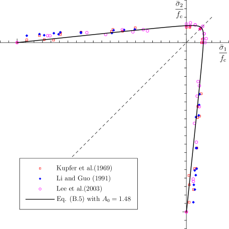
The modified von Mises criterion (2.18)₂ is recovered for the parameter $A_{0}=0$ . As an illustrative example, let us consider the typical strength ratio $\rho_{s}:=f_{\text{c}}/f_{\text{t}}=10$ for concrete. The biaxial strength envelope resulted from the following parameters

\displaystyle A_{0}=1.48\qquad\Longrightarrow\qquad B_{0}=2.34,\qquad C_{0}=0.93

(B.5)

fits the test data of normal concrete under tension-tension and tension-compression rather well; see Figure 27.