Unfolding globally resonant homoclinic tangencies.

Sishu Shankar Muni, Robert I. McLachlan, David J.W. Simpson

School of Fundamental Sciences
Massey University
Palmerston North
New Zealand

Abstract

Global resonance is a mechanism by which a homoclinic tangency of a smooth map can have infinitely many asymptotically stable, single-round periodic solutions. To understand the bifurcation structure one would expect to see near such a tangency, in this paper we study one-parameter perturbations of typical globally resonant homoclinic tangencies. We assume the tangencies are formed by the stable and unstable manifolds of saddle fixed points of two-dimensional maps. We show the perturbations display two infinite sequences of bifurcations, one saddle-node the other period-doubling, between which single-round periodic solutions are asymptotically stable. Generically these scale like $|\lambda|^{2k}$ , as $k\to\infty$ , where $-1<\lambda<1$ is the stable eigenvalue associated with the fixed point. If the perturbation is taken tangent to the surface of codimension-one homoclinic tangencies, they instead scale like $\frac{|\lambda|^{k}}{k}$ . We also show slower scaling laws are possible if the perturbation admits further degeneracies.

1 Introduction

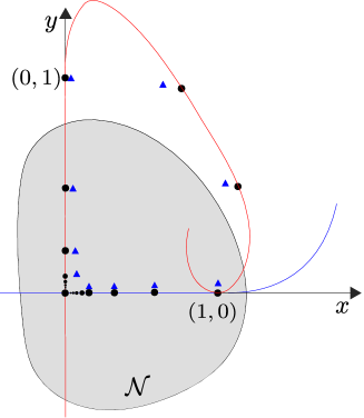
Homoclinic tangencies are perhaps the simplest mechanism in nonlinear dynamical systems for the loss of hyperbolicity and the creation of chaotic dynamics [12]. They occur most simply for saddle fixed points of two-dimensional maps. A tangential intersection between the stable and unstable manifolds of a fixed point is a homoclinic tangency, see Fig 1. This intersection is one point of an orbit that is homoclinic to the fixed point. This is a codimension-one phenomenon, meaning it can be equated to a single scalar condition. At a homoclinic tangency the map typically has infinitely many periodic solutions. Some of these are single-round, roughly meaning that they shadow the homoclinic orbit once before repeating, Fig. 1. Newhouse in [11] showed that infinitely many stable multi-round periodic solutions can coexist at a homoclinic tangency. At a generic homoclinic tangency all single-round periodic solutions of sufficiently large period are unstable [3, 4].

Refer to caption — Figure 1: A homoclinic tangency for a saddle fixed point of a two-dimensional map. In this illustration the eigenvalues associated with the fixed points are positive, i.e. $0<\lambda<1$ and $\sigma>1$ . A coordinate change has been applied so that in the region $\mathcal{N}$ (shaded) the coordinate axes coincide with the stable and unstable manifolds. The homoclinic orbit $\Gamma_{\rm HC}$ is shown with black dots. A typical single-round periodic solution is shown with blue triangles.

In our previous work [10] we determined what degeneracies are needed for the infinitely many single-round periodic solutions to be asymptotically stable for smooth maps on $\mathbb{R}^{2}$ . We found that the eigenvalues associated with the saddle fixed point, call them $\lambda$ and $\sigma$ satisfying $0<|\lambda|<1<|\sigma|$ , need to multiply to $1$ or $-1$ . If $\lambda\sigma=-1$ (so the map is orientation-reversing, at least locally), then the phenomenon is codimension-three. It involves a ‘global resonance’ condition on the reinjection mechanism for taking iterates back to a neighbourhood of the fixed point.

If a family of maps $f_{\mu}$ , with $\mu\in\mathbb{R}^{n}$ , has this phenomenon at some point $\mu^{*}$ in parameter space, then for any positive $j\in\mathbb{Z}$ there exists an open set containing $\mu^{*}$ in which $j$ asymptotically stable, single-round periodic solutions coexist. Due to the high codimension, a precise description of the shape of these sets (for large $j$ ) is beyond the scope of this paper. The approach we take here is to consider one-parameter families that perturb from a globally resonant homoclinic tangency. Some information about the size and shapes of the sets can then be inferred from our results. Globally resonant homoclinic tangencies are hubs for extreme multi-stability. They should occur generically in some families of maps with three or more parameters, such as the generalised Hénon map [8, 9], but to our knowledge they have yet to have been identified.

We find that as the value of $\mu$ is varied from $\mu^{*}$ , there occurs infinite sequence of either saddle-node or period-doubling bifurcations that destroy the periodic solutions or make them unstable. Generically these sequences converge exponentially to $\mu^{*}$ with the distance (in parameter space) to the bifurcation asymptotically proportional to $|\lambda|^{2k}$ , where the periodic solutions have period $k+m$ , for some fixed $m\geq 1$ . If we move away from $\mu^{*}$ without a linear change to the codimension-one condition of a homoclinic tangency, the bifurcation values instead generically scale like $\frac{|\lambda|^{k}}{k}$ . If the perturbation suffers further degeneracies, the scaling can be slower. Specifically we observe $|\lambda|^{k}$ and $\frac{1}{k}$ for an abstract example that we believe is representative of how the bifurcations scale in general.

Similar results have been obtained for more restrictive classes of maps. For area-preserving families the phenomenon is codimension-two and there exist infinitely many elliptic, single-round periodic solutions [7]. As shown in [1, 5] the periodic solutions are destroyed or lose stability in bifurcations that scale like $|\alpha|^{2k}$ , matching our result. For piecewise-linear families the phenomenon is codimension-three [15, 16]. In this setting the bifurcation values instead scale like $|\alpha|^{k}$ [14], see also [2].

The phenomenon is also reminscient of a celebrated result of Newhouse [11]. Newhouse showed that for a generic (codimension-one) homoclinic tangency with $|\lambda\sigma|<1$ , infinitely many asymptotically stable periodic solutions coexist for a dense set of parameter values near that of the tangency. However, in this scenario the periodic solutions are multi-round (shadow the homoclinic orbit several times before repeating).

The remainder of the paper is organised as follows. In §2 we introduce two maps, $T_{0}$ and $T_{1}$ , to describe the dynamics near the homoclinic orbit. The map $T_{0}$ is a local map describing the saddle fixed point, while $T_{1}$ represents the reinjection mechanism. The single-round periodic solutions correspond to fixed points of $T_{0}^{k}\circ T_{1}$ . In §3 we summarise the necessary and sufficient conditions derived in [10] for the coexistence of infinitely many asymptotically stable, single-round periodic solutions. Then in §4–6 we introduce parameter-dependence and state our main result (Theorem 6.1) for the scaling properties of the saddle-node and period-doubling bifurcations. A proof of Theorem 6.1 is provided in §7. Next in §8 we illustrate Theorem 6.1 with a four-parameter family of $C^{1}$ maps (an abstract minimal example). We observe numerically computed bifurcation values match those predicted by Theorem 6.1, to leading order, and observe slower scaling laws in special cases. Finally §9 provides a discussion and outlook for further studies.

2 A quantitative description of the dynamics near a homoclinic connection

Let $f$ be a $C^{\infty}$ map on $\mathbb{R}^{2}$ . Suppose the origin $(x,y)=(0,0)$ is a saddle fixed point of $f$ . That is, ${\rm D}f(0,0)$ has eigenvalues $\lambda,\sigma\in\mathbb{R}$ satisfying

0<|\lambda|<1<|\sigma|.

(2.1)

By the results of Sternberg [13, 17] there exists a $C^{\infty}$ coordinate change that transforms $f$ to

T_{0}(x,y)=\begin{bmatrix}\lambda x\mathopen{}\mathclose{{}\left(1+\mathcal{O}\mathopen{}\mathclose{{}\left(xy}\right)}\right)\\ \sigma y\mathopen{}\mathclose{{}\left(1+\mathcal{O}\mathopen{}\mathclose{{}\left(xy}\right)}\right)\end{bmatrix}.

(2.2)

In these new coordinates let $\mathcal{N}$ be a convex neighbourhood of the origin for which

f(x,y)=T_{0}(x,y),\qquad\text{for all $(x,y)\in\mathcal{N}$}.

(2.3)

See Fig. 1. If $\lambda^{p}\sigma^{q}\neq 1$ for all integers $p,q\geq 1$ , then the eigenvalues are said to be non-resonant and the coordinate change can be chosen so that $T_{0}$ is linear. If not, then $T_{0}$ must contain resonant terms that cannot be eliminated by the coordinate change. As explained in §4, if $\lambda\sigma=1$ we can reach the form

T_{0}(x,y)=\begin{bmatrix}\lambda x\mathopen{}\mathclose{{}\left(1+a_{1}xy+\mathcal{O}\mathopen{}\mathclose{{}\left(x^{2}y^{2}}\right)}\right)\\ \sigma y\mathopen{}\mathclose{{}\left(1+b_{1}xy+\mathcal{O}\mathopen{}\mathclose{{}\left(x^{2}y^{2}}\right)}\right)\end{bmatrix},

(2.4)

where $a_{1},b_{1}\in\mathbb{R}$ . If $\lambda\sigma=-1$ we can obtain (2.4) with $a_{1}=b_{1}=0$ .

Now suppose there exists an orbit homoclinic to the origin, $\Gamma_{\rm HC}$ . By scaling $x$ and $y$ we may assume that $(1,0)$ and $(0,1)$ are points on $\Gamma_{\rm HC}$ and

(1,0),(\lambda,0),\mathopen{}\mathclose{{}\left(0,\tfrac{1}{\sigma}}\right),\mathopen{}\mathclose{{}\left(0,\tfrac{1}{\sigma^{2}}}\right)\in\mathcal{N},

(2.5)

By assumption there exists $m\geq 1$ such that $f^{m}(0,1)=(1,0)$ . We let $T_{1}=f^{m}$ and expand $T_{1}$ in a Taylor series centred at $(x,y)=(0,1)$ :

T_{1}(x,y)=\begin{bmatrix}c_{0}+c_{1}x+c_{2}(y-1)+\mathcal{O}\mathopen{}\mathclose{{}\left((x,y-1)^{2}}\right)\\ d_{0}+d_{1}x+d_{2}(y-1)+d_{3}x^{2}+d_{4}x(y-1)+d_{5}(y-1)^{2}+\mathcal{O}\mathopen{}\mathclose{{}\left((x,y-1)^{3}}\right)\end{bmatrix},

(2.6)

where $c_{0}=1$ and $d_{0}=0$ . In (2.6) we have written explicitly the terms that will be important below.

3 Conditions for infinitely many stable single-round solutions

In this section we state the main results of our previous work [10]. First Theorem 3.4 gives necessary conditions for the existence of infinitely many stable, single-round periodic solutions. Then Theorem 3.2 gives sufficient conditions for these to exist and be asymptotically stable.

Theorem 3.1.

Suppose $f$ satisfies (2.3) with (2.2) and (2.5). Suppose in (2.6) we have $c_{0}=1$ , $d_{0}=0$ , $d_{5}\neq 0$ , and $c_{1}d_{2}-c_{2}d_{1}\neq 0$ . Suppose $f$ has an infinite sequence of stable, single-round, periodic solutions accumulating on $\Gamma_{\rm HC}$ . Then

$\displaystyle d_{2}$	$\displaystyle=0,$	(3.1)
$\displaystyle\|\lambda\sigma\|$	$\displaystyle=1,$	(3.2)
$\displaystyle\|d_{1}\|$	$\displaystyle=1,$	(3.3)

with $d_{1}=1$ in the case $\lambda\sigma=1$ . Moreover, if $\lambda\sigma=1$ and $T_{0}$ has the form (2.4) then

a_{1}+b_{1}=0.

(3.4)

The equation $d_{2}=0$ corresponds to a homoclinic tangency, as shown in Fig. 1. With $|\lambda\sigma|=1$ we have $|\det({\rm D}f)|=1$ at the origin. The condition $d_{1}=1$ is a global condition, see [10] for a geometric interpretation, with which the tangency is termed globally resonant. Finally if $\lambda\sigma=1$ and $T_{0}$ has the form (2.4), then $\det({\rm D}f)=1+2(a_{1}+b_{1})xy+\mathcal{O}\mathopen{}\mathclose{{}\left(x^{2}y^{2}}\right)$ . Thus the condition $a_{1}+b_{1}=0$ implies that as $(x,y)$ is varied from $(0,0)$ , the value of $\det({\rm D}f)$ varies quadratically instead of linearly (as is generically the case). Now suppose $|\lambda\sigma|=1$ . Given $k_{\rm min}\in\mathbb{Z}$ , let

K(k_{\rm min})=\mathopen{}\mathclose{{}\left\{k\in\mathbb{Z}\,\big{|}\,k\geq k_{\rm min},\mathopen{}\mathclose{{}\left(\lambda\sigma}\right)^{k}=d_{1}}\right\}.

(3.5)

If $\lambda\sigma=d_{1}=1$ , then $K$ is the set of all integers greater than or equal to $k_{\rm min}$ . If $\lambda\sigma=-1$ and $d_{1}=1$ [resp. $d_{1}=-1$ ], then $K$ is the set of all even [resp. odd] integers greater than or equal to $k_{\rm min}$ . Also let

\Delta=\mathopen{}\mathclose{{}\left(1-c_{2}-d_{1}d_{4}}\right)^{2}-4d_{5}(d_{3}+c_{1}d_{1}).

(3.6)

Theorem 3.2.

Suppose $f$ satisfies (2.3) with (2.4) and (2.5). Suppose $c_{0}=1$ , $d_{0}=0$ , and $d_{5}\neq 0$ . Suppose (3.1)–(3.4) are satisfied, $\Delta>0$ , and

-1<c_{2}<1-\frac{\sqrt{\Delta}}{2}.

(3.7)

Then there exists $k_{\rm min}\in\mathbb{Z}$ such that $f$ has an asymptotically stable period- $(k+m)$ solution for all $k\in K(k_{\rm min})$ .

Theorems 3.4 and 3.2 imply that the phenomenon of infinitely many asymptotically stable, single-round periodic solutions is codimension-three in the case $\lambda\sigma=-1$ . Specifically the three independent codimension-one conditions (3.1)–(3.3) need to hold, and the phenomenon indeed occurs if $\Delta>0$ and (3.7) holds. In the case $\lambda\sigma=1$ the phenomenon is codimension-four as we also require (3.4). This condition is absent when $\lambda\sigma=-1$ because in this case the cubic terms in (2.4) are removable.

4 Smooth parameter dependence

Now suppose $f_{\mu}$ is a $C^{\infty}$ map on $\mathbb{R}^{2}$ with a $C^{\infty}$ dependence on a parameter $\mu\in\mathbb{R}^{n}$ . Let ${\bf 0}\in\mathbb{R}^{n}$ denote the origin in parameter space. Suppose that for all $\mu$ in some region containing ${\bf 0}$ , the origin in phase space $(x,y)=(0,0)$ is a fixed point of $f_{\mu}$ . Let $\lambda=\lambda(\mu)$ and $\sigma=\sigma(\mu)$ be its associated eigenvalues (these are $C^{\infty}$ functions of $\mu$ ) and suppose

	$\displaystyle\lambda({\bf 0})$	$\displaystyle=\alpha,$		(4.1)
	$\displaystyle\sigma({\bf 0})$	$\displaystyle=\frac{\chi_{\rm eig}}{\alpha},$		(4.2)

with $0<\alpha<1$ and $\chi_{\rm eig}\in\{-1,1\}$ . With $\mu={\bf 0}$ we have $|\lambda\sigma|=1$ , so as described above $T_{0}$ can be assumed to have the form (2.4). We now show we can assume $T_{0}$ has this form when the value of $\mu$ is sufficiently small.

Lemma 4.1.

There exists a neighbourhood $\mathcal{N}_{\rm param}\subset\mathbb{R}^{n}$ of ${\bf 0}$ and a $C^{\infty}$ coordinate change that puts $f_{\mu}$ in the form (2.4) for all $\mu\in\mathcal{N}_{\rm param}$ .

Proof.

Via a linear transformation $f_{\mu}$ can be transformed to

\begin{bmatrix}x\\ y\end{bmatrix}\mapsto\begin{bmatrix}\lambda x+\sum\limits_{i\geq 0,\,j\geq 0,\,i+j\geq 2}a_{ij}x^{i}y^{j}\\ \sigma y+\sum\limits_{i\geq 0,\,j\geq 0,\,i+j\geq 2}b_{ij}x^{i}y^{j}\end{bmatrix},

for some $a_{ij},b_{ij}\in\mathbb{R}$ . It is a standard asymptotic matching exercise to show that via an additional $C^{\infty}$ coordinate change we can achieve $a_{ij}=0$ if $\lambda^{i-1}\sigma^{j}\neq 1$ , and $b_{ij}=0$ if $\lambda^{i}\sigma^{j-1}\neq 1$ . The remainder of the proof is based on this fact.

Assume the value of $\mu$ is small enough that (2.1) is satisfied. Then $\lambda^{p}\sigma^{q}=1$ is only possible with $p,q\geq 1$ , so a $C^{\infty}$ coordinate change can be performed to reduce the map to

\begin{bmatrix}x\\ y\end{bmatrix}\mapsto\begin{bmatrix}\lambda x+\sum\limits_{i\geq 2,\,j\geq 1}a_{ij}x^{i}y^{j}\\ \sigma y+\sum\limits_{i\geq 1,\,j\geq 2}b_{ij}x^{i}y^{j}\end{bmatrix}.

Since $|\lambda\sigma|=1$ when $\mu={\bf 0}$ we can assume $\mu$ is small enough that $\lambda^{p-1}\sigma\neq 1$ for all $p\geq 3$ and $\lambda\sigma^{q-1}\neq 1$ for all $q\geq 3$ . Consequently the map can further be reduced to

\begin{bmatrix}x\\ y\end{bmatrix}\mapsto\begin{bmatrix}\lambda x+a_{21}x^{2}y+\sum\limits_{i\geq 3,\,j\geq 2}a_{ij}x^{i}y^{j}\\ \sigma y+b_{12}xy^{2}+\sum\limits_{i\geq 2,\,j\geq 3}b_{ij}x^{i}y^{j}\end{bmatrix},

which can be rewritten as (2.4). ∎

The product of the eigenvalues is

\lambda(\mu)\sigma(\mu)=\chi_{\rm eig}+{\bf n}_{\rm eig}^{\sf T}\mu+\mathcal{O}\mathopen{}\mathclose{{}\left(\|\mu\|^{2}}\right),

(4.3)

where ${\bf n}_{\rm eig}$ is the gradient of $\lambda\sigma$ evaluated at $\mu={\bf 0}$ . The following result is an elementary application of the implicit function theorem.

Lemma 4.2.

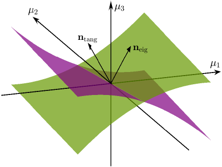
Suppose ${\bf n}_{\rm eig}\neq{\bf 0}$ . Then $|\lambda(\mu)\sigma(\mu)|=1$ on a $C^{\infty}$ codimension-one surface intersecting $\mu={\bf 0}$ and with normal vector ${\bf n}_{\rm eig}$ at $\mu={\bf 0}$ (as illustrated in Fig. 2).

5 The codimension-one surface of homoclinic tangencies

In this section we describe the codimension-one surface of homoclinic tangencies that intersects $\mu={\bf 0}$ where we will be assuming that a globally resonant homoclinic tangency occurs.

Suppose (2.5) is satisfied when $\mu={\bf 0}$ . Write $f_{\mu}^{m}$ as (2.6) and suppose

	$\displaystyle c_{0}({\bf 0})$	$\displaystyle=1,$		(5.1)
	$\displaystyle d_{0}({\bf 0})$	$\displaystyle=0,$		(5.2)

so that $f_{\bf 0}$ has an orbit homoclinic to the origin through $(x,y)=(1,0)$ and $(0,1)$ . Also suppose

	$\displaystyle d_{2}({\bf 0})$	$\displaystyle=0,$		(5.3)
	$\displaystyle d_{5}({\bf 0})$	$\displaystyle=d_{5,0}\neq 0,$		(5.4)

for a quadratic tangency. Also write

d_{0}(\mu)={\bf n}_{\rm tang}^{\sf T}\mu+\mathcal{O}\mathopen{}\mathclose{{}\left(\|\mu\|^{2}}\right).

(5.5)

Lemma 5.1.

Suppose (2.5) is satisfied when $\mu={\bf 0}$ , (5.1)–(5.4) are satisfied, and ${\bf n}_{\rm tang}\neq{\bf 0}$ . Then $f_{\mu}$ has a quadratic homoclinic tangency to $(x,y)=(0,0)$ on a $C^{\infty}$ codimension-one surface intersecting $\mu={\bf 0}$ and with normal vector ${\bf n}_{\rm tang}$ at $\mu={\bf 0}$ . Moreover, this tangency occurs at $(x,y)=(0,Y(\mu))$ where $Y$ is a $C^{\infty}$ function with $Y({\bf 0})=1$ .

Proof.

Let $T_{1,2}$ denote the second component of $T_{1}$ (2.6). The function

h(u;\mu)=\frac{\partial T_{1,2}}{\partial y}(0,1+u)=d_{2}(\mu)+2d_{5}(\mu)u+\mathcal{O}(2),

is a $C^{\infty}$ function of $u\in\mathbb{R}$ and $\mu$ . Since $h(0;\mathbf{0})=0$ by (5.3) and $\frac{\partial h}{\partial u}(0;\mathbf{0})\neq 0$ by (5.4), the implicit function theorem implies there exists a $C^{\infty}$ function $u_{\rm tang}(\mu)$ such that $h(u_{\rm tang}(\mu);\mu)=0$ locally.

By construction, the unstable manifold of $(x,y)=(0,0)$ is tangent to the $x$ -axis at $T_{1}(0,1+u_{\rm tang})$ . Moreover this tangency is quadratic by (5.4). Thus a homoclinic tangency occurs if $T_{1,2}(0,1+u_{\rm tang})=d_{0}+d_{2}u_{\rm tang}+d_{5}u_{\rm tang}^{2}+\mathcal{O}(3)=0$ . This function is $C^{\infty}$ and

T_{1,2}(0,1+u_{\rm tang})={\bf n}_{\rm tang}^{\sf T}\mu+\mathcal{O}\mathopen{}\mathclose{{}\left(\|\mu\|^{2}}\right).

Since ${\bf n}_{\rm tang}\neq{\bf 0}$ the result follows from another application of the implicit function theorem. ∎

6 Sequences of saddle-node and period-doubling bifurcations

Suppose

d_{1}({\bf 0})=\chi,

(6.1)

where $\chi\in\{-1,1\}$ . Write

	$\displaystyle a_{1}({\bf 0})$	$\displaystyle=a_{1,0}\,,$	$\displaystyle\qquad c_{1}({\bf 0})$	$\displaystyle=c_{1,0}\,,$	$\displaystyle\qquad d_{3}({\bf 0})$	$\displaystyle=d_{3,0}\,,$		(6.2)
	$\displaystyle b_{1}({\bf 0})$	$\displaystyle=b_{1,0}\,,$	$\displaystyle\qquad c_{2}({\bf 0})$	$\displaystyle=c_{2,0}\,,$	$\displaystyle\qquad d_{4}({\bf 0})$	$\displaystyle=d_{4,0}\,,$		(6.2)

and, recalling (3.6), let

\Delta_{0}=\mathopen{}\mathclose{{}\left(1-c_{2,0}-\chi d_{4,0}}\right)^{2}-4d_{5,0}(d_{3,0}+\chi c_{1,0}).

(6.3)

Theorem 6.1.

Suppose $f_{\mu}$ satisfies (4.1), (4.2), (5.1)–(5.4), $a_{1,0}+b_{1,0}=0$ , $\Delta_{0}>0$ , and $-1<c_{2,0}<1-\frac{\sqrt{\Delta_{0}}}{2}$ . Let ${\bf v}\in\mathbb{R}^{n}$ . If ${\bf n}_{\rm tang}^{\sf T}{\bf v}\neq 0$ then there exists $k_{\rm min}\in\mathbb{Z}$ such that for all $k\in K(k_{\rm min})$ there exist $\varepsilon_{k}^{-}<0$ and $\varepsilon_{k}^{+}>0$ with $\varepsilon_{k}^{\pm}=\mathcal{O}\mathopen{}\mathclose{{}\left(\alpha^{2k}}\right)$ such that $f$ has an asymptotically stable period- $(k+m)$ solution for all $\mu=\varepsilon{\bf v}$ with $\varepsilon_{k}^{-}<\varepsilon<\varepsilon_{k}^{+}$ . Moreover, one sequence, $\{\varepsilon_{k}^{-}\}$ or $\{\varepsilon_{k}^{+}\}$ , corresponds to saddle-node bifurcations of the periodic solutions, the other to period-doubling bifurcations. If instead ${\bf n}_{\rm tang}^{\sf T}{\bf v}=0$ and ${\bf n}_{\rm eig}^{\sf T}{\bf v}\neq 0$ the same results hold now $\varepsilon_{k}^{\pm}=\mathcal{O}\mathopen{}\mathclose{{}\left(\frac{\alpha^{k}}{k}}\right)$ .

7 Proof of the main result

To prove Theorem 6.1 we use the following lemma which is proved in Appendix A by carefully estimating the error terms in (7.1).. If $\chi_{\rm eig}=-1$ then (7.1) is true if $a_{1}=b_{1}=0$ (and this can be proved in the same fashion).

Lemma 7.1.

Suppose $\chi_{\rm eig}=1$ and $\mu=\mathcal{O}\mathopen{}\mathclose{{}\left(\alpha^{k}}\right)$ . If $|x-1|$ and $\mathopen{}\mathclose{{}\left|\alpha^{-k}y-1}\right|$ are sufficiently small for all sufficiently large values of $k$ , then

T_{0}^{k}(x,y)=\begin{bmatrix}\lambda^{k}x\mathopen{}\mathclose{{}\left(1+ka_{1}xy+\mathcal{O}\mathopen{}\mathclose{{}\left(k^{2}\alpha^{2k}}\right)}\right)\\ \sigma^{k}y\mathopen{}\mathclose{{}\left(1+kb_{1}xy+\mathcal{O}\mathopen{}\mathclose{{}\left(k^{2}\alpha^{2k}}\right)}\right)\end{bmatrix}.

(7.1)

Proof of Theorem 6.1.

Step 1 — Coordinate changes to distinguish the surface of homoclinic tangencies.
First we perform two coordinate changes on parameter space. There exists an $n\times n$ orthogonal matrix $A$ such that after $\mu$ is replaced with $A\mu$ , and $\mu$ is scaled, we have ${\bf n}_{\rm tang}^{\sf T}=[1,0,\ldots,0]$ — the first coordinate vector of $\mathbb{R}^{n}$ . Then $d_{0}(\mu)=\mu_{1}+\mathcal{O}\mathopen{}\mathclose{{}\left(\|\mu\|^{2}}\right)$ . Second, for convenience, we apply a near-identity transformation to remove the higher order terms, resulting in

d_{0}(\mu)=\mu_{1}\,.

(7.2)

These coordinate changes do not alter the signs of the dot products ${\bf n}_{\rm tang}^{\sf T}{\bf v}$ and ${\bf n}_{\rm eig}^{\sf T}{\bf v}$ . Now write

$\displaystyle c_{0}(\mu)$	$\displaystyle=1+\sum_{i=1}^{n}p_{i}\mu_{i}+\mathcal{O}\mathopen{}\mathclose{{}\left(\\|\mu\\|^{2}}\right),$	(7.3)
$\displaystyle d_{1}(\mu)$	$\displaystyle=\chi+\sum_{i=1}^{n}q_{i}\mu_{i}+\mathcal{O}\mathopen{}\mathclose{{}\left(\\|\mu\\|^{2}}\right),$	(7.4)
$\displaystyle d_{2}(\mu)$	$\displaystyle=\sum_{i=1}^{n}r_{i}\mu_{i}+\mathcal{O}\mathopen{}\mathclose{{}\left(\\|\mu\\|^{2}}\right),$	(7.5)

	$\displaystyle\lambda(\mu)$	$\displaystyle=\alpha+\sum_{i=1}^{n}s_{i}\mu_{i}+\mathcal{O}\mathopen{}\mathclose{{}\left(\\|\mu\\|^{2}}\right),$		(7.6)
	$\displaystyle\sigma(\mu)$	$\displaystyle=\frac{\chi_{\rm eig}}{\alpha}+\sum_{i=1}^{n}t_{i}\mu_{i}+\mathcal{O}\mathopen{}\mathclose{{}\left(\\|\mu\\|^{2}}\right),$		(7.7)

where $p_{i},\ldots,t_{i}\in\mathbb{R}$ are constants. Step 2 — Apply a $k$ -dependent scaling to $\mu$ .
In view of the coordinate changes applied in the previous step, the surface of homoclinic surfaces of Lemma 5.1 is tangent to the $\mu_{1}=0$ coordinate hyperplane. In order to show that bifurcation values scale like $|\alpha|^{2k}$ if we adjust the value of $\mu$ in a direction transverse to this surface, and, generically, scale like $\frac{|\alpha|^{k}}{k}$ otherwise, we scale the components of $\mu$ as follows:

\mu_{i}=\begin{cases}\alpha^{2k}\tilde{\mu}_{i}\,,&i=1,\\ \alpha^{k}\tilde{\mu}_{i}\,,&i\neq 1.\end{cases}

(7.8)

Below we will see that the resulting asymptotic expansions are consistent and this will justify (7.8). Notice that $\tilde{\mu}_{1}$ -terms are higher order than $\tilde{\mu}_{i}$ -terms, for $i\neq 1$ . For example (7.6) now becomes $\lambda=\alpha+\sum_{i=2}^{n}s_{i}\tilde{\mu}_{i}\alpha^{k}+\mathcal{O}\mathopen{}\mathclose{{}\left(|\alpha|^{2k}}\right)$ . Further, let $k$ be such that $\lambda({\bf 0})^{k}\sigma({\bf 0})^{k}=d_{1}({\bf 0})$ , that is $\chi_{\rm eig}^{k}=\chi$ . Then from (7.6)–(7.8) we obtain

	$\displaystyle\lambda^{k}$	$\displaystyle=\alpha^{k}\mathopen{}\mathclose{{}\left(1+\frac{k}{\alpha}\sum_{i=2}^{n}s_{i}\tilde{\mu}_{i}\alpha^{k}+\mathcal{O}\mathopen{}\mathclose{{}\left(k^{2}\|\alpha\|^{2k}}\right)}\right),$		(7.9)
	$\displaystyle\sigma^{k}$	$\displaystyle=\frac{\chi}{\alpha^{k}}\mathopen{}\mathclose{{}\left(1+k\alpha\chi_{\rm eig}\sum_{i=2}^{n}t_{i}\tilde{\mu}_{i}\alpha^{k}+\mathcal{O}\mathopen{}\mathclose{{}\left(k^{2}\|\alpha\|^{2k}}\right)}\right).$		(7.10)

Step 3 — Calculate one point of each periodic solution.
One point of a single-round periodic solution is a fixed point of $T_{0}^{k}\circ T_{1}$ . We look for fixed points $\mathopen{}\mathclose{{}\left(x^{(k)},y^{(k)}}\right)$ of $T_{0}^{k}\circ T_{1}$ of the form

\begin{split}x^{(k)}&=\alpha^{k}\mathopen{}\mathclose{{}\left(1+\phi_{k}\alpha^{k}+\mathcal{O}\mathopen{}\mathclose{{}\left(k^{2}|\alpha|^{2k}}\right)}\right),\\ y^{(k)}&=1+\psi_{k}\alpha^{k}+\mathcal{O}\mathopen{}\mathclose{{}\left(k^{2}|\alpha|^{2k}}\right).\end{split}

(7.12)

By substituting (7.12) into (2.6) and the above various asymptotic expressions for the coefficients in $T_{1}$ , we obtain

T_{1}\mathopen{}\mathclose{{}\left(x^{(k)},y^{(k)}}\right)=\begin{bmatrix}1+\mathopen{}\mathclose{{}\left(c_{1,0}+c_{2,0}\psi_{k}+\sum_{i=2}^{n}p_{i}\tilde{\mu}_{i}}\right)\alpha^{k}+\mathcal{O}\mathopen{}\mathclose{{}\left(k^{2}|\alpha|^{2k}}\right)\\ \begin{aligned} \chi\alpha^{k}+\mathopen{}\mathclose{{}\left(\tilde{\mu}_{1}+d_{3,0}+d_{4,0}\psi_{k}+d_{5,0}\psi_{k}^{2}+\chi\phi_{k}+\sum_{i=2}^{n}\mathopen{}\mathclose{{}\left(q_{i}+r_{i}\psi_{k}}\right)\tilde{\mu}_{i}}\right)\alpha^{2k}&\\[5.69054pt] +\mathcal{O}\mathopen{}\mathclose{{}\left(k^{2}|\alpha|^{3k}}\right)&\end{aligned}\end{bmatrix}.

Then by (7.1),

\mathopen{}\mathclose{{}\left(T_{0}^{k}\circ T_{1}}\right)\mathopen{}\mathclose{{}\left(x^{(k)},y^{(k)}}\right)=\begin{bmatrix}\begin{aligned} \alpha^{k}+\bigg{(}a_{1,0}\chi+\frac{1}{\alpha}\sum_{i=2}^{n}s_{i}\tilde{\mu}_{i}\bigg{)}k\alpha^{2k}+\bigg{(}c_{1,0}+c_{2,0}\psi_{k}+\sum_{i=2}^{n}p_{i}\tilde{\mu}_{i}\bigg{)}\alpha^{2k}&\\[5.69054pt] +\mathcal{O}\mathopen{}\mathclose{{}\left(k^{2}|\alpha|^{3k}}\right)&\end{aligned}\\ \begin{aligned} 1+\bigg{(}b_{1,0}\chi+\alpha\chi_{\rm eig}\sum_{i=2}^{n}t_{i}\tilde{\mu}_{i}\bigg{)}k\alpha^{k}+\bigg{(}\chi\tilde{\mu}_{1}+\chi d_{3,0}+\chi d_{4,0}\psi_{k}&\\ +\chi d_{5,0}\psi_{k}^{2}+\phi_{k}+\chi\sum_{i=2}^{n}\mathopen{}\mathclose{{}\left(q_{i}+r_{i}\psi_{k}}\right)\tilde{\mu}_{i}\bigg{)}\alpha^{k}+\mathcal{O}\mathopen{}\mathclose{{}\left(k^{2}|\alpha|^{2k}}\right)&\end{aligned}\end{bmatrix}.

(7.13)

By matching (7.12) and (7.13) and eliminating $\phi_{k}$ we obtain the following expression that determines the possible values of $\psi_{k}$ :

\chi d_{5,0}\psi_{k}^{2}-P\psi_{k}+Q=0,

(7.14)

where

	$\displaystyle P$	$\displaystyle=1-c_{2,0}-\chi d_{4,0}-\chi\sum_{i=2}^{n}r_{i}\tilde{\mu}_{i}\,,$		(7.15)
	$\displaystyle Q$	$\displaystyle=\chi\tilde{\mu}_{1}+c_{1,0}+\chi d_{3,0}+\sum_{i=2}^{n}\mathopen{}\mathclose{{}\left(p_{i}+\chi q_{i}}\right)\tilde{\mu}_{i}+\sum_{i=2}^{n}\mathopen{}\mathclose{{}\left(\frac{s_{i}}{\alpha}+\alpha\chi_{\rm eig}t_{i}}\right)\tilde{\mu}_{i}k,$		(7.16)

and we have also used $a_{1,0}+b_{1,0}=0$ . Of the two solutions to (7.14), the one that yields an asymptotically stable solution when $\mu={\bf 0}$ is

\psi_{k}=\frac{1}{2\chi d_{5,0}}\mathopen{}\mathclose{{}\left(P-\sqrt{P^{2}-4\chi d_{5,0}Q}}\right).

(7.17)

Note that this solution exists and is real-valued for sufficiently small values of $\mu$ because when $\mu={\bf 0}$ the discriminant is $P^{2}-4\chi d_{5,0}Q=\Delta_{0}>0$ .

Step 4 — Stability of the periodic solution.
By using (2.6), (7.1), (7.9), (7.10), and (7.12),

{\rm D}\mathopen{}\mathclose{{}\left(T_{0}^{k}\circ T_{1}}\right)\mathopen{}\mathclose{{}\left(x^{(k)},y^{(k)}}\right)=\begin{bmatrix}\mathcal{O}\mathopen{}\mathclose{{}\left(|\alpha|^{k}}\right)&c_{2,0}\alpha^{k}+\mathcal{O}\mathopen{}\mathclose{{}\left(k|\alpha|^{2k}}\right)\\ \frac{1}{\alpha^{k}}\mathopen{}\mathclose{{}\left(1+\mathcal{O}\mathopen{}\mathclose{{}\left(k|\alpha|^{k}}\right)}\right)&\chi d_{4,0}+\chi\sum_{i=2}^{n}r_{i}\tilde{\mu}_{i}+2\chi d_{5,0}\psi_{k}+\mathcal{O}\mathopen{}\mathclose{{}\left(k|\alpha|^{k}}\right)\end{bmatrix}.

(7.18)

Let $\tau_{k}$ and $\delta_{k}$ denote the trace and determinant of this matrix, respectively. By (7.15), (7.17), and (7.18) we obtain

	$\displaystyle\tau_{k}$	$\displaystyle=1-c_{2,0}-\sqrt{P^{2}-4\chi d_{5,0}Q}+\mathcal{O}\mathopen{}\mathclose{{}\left(k\|\alpha\|^{k}}\right),$		(7.19)
	$\displaystyle\delta_{k}$	$\displaystyle=-c_{2,0}+\mathcal{O}\mathopen{}\mathclose{{}\left(k\|\alpha\|^{k}}\right).$		(7.20)

By substituting $\mu={\bf 0}$ into (7.19) we obtain $\tau_{k}=1-c_{2,0}-\sqrt{\Delta_{0}}$ . It immediately follows from the assumption $-1<c_{2,0}<1-\frac{\sqrt{\Delta_{0}}}{2}$ that the periodic solution is asymptotically stable for sufficiently large values of $k$ .

Step 5 — The generic case ${\bf n}_{\rm tang}^{\sf T}{\bf v}\neq 0$ .
Now suppose ${\bf n}_{\rm tang}^{\sf T}{\bf v}\neq 0$ , that is, $v_{1}\neq 0$ (in view of the earlier coordinate change). Write $\mu=\varepsilon{\bf v}$ and $\varepsilon=\tilde{\varepsilon}\alpha^{2k}$ . By (7.8), $\tilde{\mu}_{1}=\tilde{\varepsilon}v_{1}$ and $\tilde{\mu}_{i}=\tilde{\varepsilon}v_{i}\alpha^{k}$ for $i\neq 1$ . Then by (7.15) and (7.16), $P=1-c_{2,0}-\chi d_{4,0}+\mathcal{O}\mathopen{}\mathclose{{}\left(|\alpha|^{k}}\right)$ and $Q=c_{1,0}+\chi d_{3,0}+\chi\tilde{\varepsilon}v_{1}+\mathcal{O}\mathopen{}\mathclose{{}\left(|\alpha|^{k}}\right)$ , so

P^{2}-4\chi d_{5,0}Q=\mathopen{}\mathclose{{}\left(1-c_{2,0}-\chi d_{4,0}}\right)^{2}-4\chi d_{5,0}\mathopen{}\mathclose{{}\left(c_{1,0}+\chi d_{3,0}+\chi\tilde{\varepsilon}v_{1}}\right)+\mathcal{O}\mathopen{}\mathclose{{}\left(|\alpha|^{k}}\right).

(7.21)

Since $v_{1}\neq 0$ and $d_{5,0}\neq 0$ we can solve $\delta_{k}-\tau_{k}+1=0$ for $\tilde{\varepsilon}$ (formally this is achieved via the implicit function theorem) and the solution is

\tilde{\varepsilon}_{\rm SN}=\frac{\Delta_{0}}{4d_{5,0}v_{1}}+\mathcal{O}\mathopen{}\mathclose{{}\left(k|\alpha|^{k}}\right).

(7.22)

Also we can use (7.21) to solve $\delta_{k}+\tau_{k}+1=0$ for $\tilde{\varepsilon}$ :

\tilde{\varepsilon}_{\rm PD}=\frac{\Delta_{0}-4\mathopen{}\mathclose{{}\left(1-c_{2,0}}\right)^{2}}{4d_{5,0}v_{1}}+\mathcal{O}\mathopen{}\mathclose{{}\left(k|\alpha|^{k}}\right).

(7.23)

Since $\tilde{\varepsilon}_{\rm SN}$ and $\tilde{\varepsilon}_{\rm PD}$ evidently have opposite signs, this completes the proof in the first case.

Step 6 — The degenerate case ${\bf n}_{\rm tang}^{\sf T}{\bf v}=0$ .
Now suppose $v_{1}=0$ and ${\bf n}_{\rm eig}^{\sf T}{\bf v}\neq 0$ . Again write $\mu=\varepsilon{\bf v}$ but now write $\varepsilon=\frac{\tilde{\varepsilon}\alpha^{k}}{k}$ . By (7.8), $\tilde{\mu}_{1}=0$ and $\tilde{\mu}_{i}=\frac{\tilde{\varepsilon}v_{i}}{k}$ for $i\neq 1$ .

We first evaluate ${\bf n}_{\rm eig}^{\sf T}{\bf v}$ . By multiplying (7.6) and (7.7) and comparing the result to (4.3) we see that the $i^{\rm th}$ element of ${\bf n}_{\rm eig}$ is $\frac{\chi_{\rm eig}s_{i}}{\alpha}+\alpha t_{i}$ . Then since $v_{1}=0$ we have ${\bf n}_{\rm eig}^{\sf T}{\bf v}=\sum_{i=2}^{n}\mathopen{}\mathclose{{}\left(\frac{\chi_{\rm eig}s_{i}}{\alpha}+\alpha t_{i}}\right)v_{i}$ . Further, $\mu=\varepsilon{\bf v}$ and $\varepsilon=\frac{\tilde{\varepsilon}\alpha^{k}}{k}$ ,

\chi_{\rm eig}\tilde{\varepsilon}{\bf n}_{\rm eig}^{\sf T}{\bf v}=\sum_{i=2}^{n}\mathopen{}\mathclose{{}\left(\frac{s_{i}}{\alpha}+\alpha\chi_{\rm eig}t_{i}}\right)\tilde{\mu}_{i}k,

which is a term appearing in (7.16). So by (7.15) and (7.16), $P=1-c_{2,0}-\chi d_{4,0}+\mathcal{O}\mathopen{}\mathclose{{}\left(\frac{1}{k}}\right)$ and $Q=c_{1,0}+\chi d_{3,0}+\frac{\tilde{\varepsilon}\chi_{\rm eig}{\bf n}_{\rm eig}^{\sf T}{\bf v}}{k}+\mathcal{O}\mathopen{}\mathclose{{}\left(\frac{1}{k}}\right)$ . By solving $\delta_{k}-\tau_{k}+1=0$ ,

\tilde{\varepsilon}_{\rm SN}=\frac{\Delta_{0}}{4d_{5,0}\chi\chi_{\rm eig}{\bf n}_{\rm eig}^{\sf T}{\bf v}}+\mathcal{O}\mathopen{}\mathclose{{}\left(\frac{1}{k}}\right),

(7.24)

and by solving $\delta_{k}-\tau_{k}+1=0$ ,

\tilde{\varepsilon}_{\rm PD}=\frac{\Delta_{0}-4\mathopen{}\mathclose{{}\left(1-c_{2,0}}\right)^{2}}{4d_{5,0}\chi\chi_{\rm eig}{\bf n}_{\rm eig}^{\sf T}{\bf v}}+\mathcal{O}\mathopen{}\mathclose{{}\left(\frac{1}{k}}\right).

(7.25)

∎

As in the previous case, $\tilde{\varepsilon}_{\rm SN}$ and $\tilde{\varepsilon}_{\rm PD}$ have opposite signs, and this completes the proof in the second case. Notice how the assumptions we have made ensure the denominators of (7.24) and (7.25) are nonzero.

8 A comparison to numerically computed bifurcation values.

Here we extend the example given in [10] and illustrate the results with the following $C^{1}$ family of maps

f(x,y)=\begin{cases}U_{0}(x,y),&y\leq\frac{2\alpha+1}{3},\\ (1-r(y))U_{0}(x,y)+r(y)U_{1}(x,y),&\frac{2\alpha+1}{3}\leq y\leq\frac{\alpha+2}{3},\\ U_{1}(x,y),&y\geq\frac{\alpha+2}{3},\end{cases}

(8.1)

where

$\displaystyle U_{0}(x,y)$	$\displaystyle=\begin{bmatrix}(\alpha+\mu_{2})x\big{(}1+(a_{1,0}+\mu_{4})xy\big{)}\\ \frac{1}{\alpha}y(1-a_{1,0}xy)\end{bmatrix},$	(8.2)
$\displaystyle U_{1}(x,y)$	$\displaystyle=\begin{bmatrix}1+c_{2,0}(y-1)\\ \mu_{1}+(1+\mu_{3})x+d_{5,0}(y-1)^{2}\end{bmatrix},$	(8.3)
$\displaystyle r(y)$	$\displaystyle=s\mathopen{}\mathclose{{}\left(\frac{y-h_{0}}{h_{1}-h_{0}}}\right),$	(8.4)

where

s(z)=3z^{2}-2z^{3},\\

(8.5)

Below we fix

\begin{split}\alpha&=0.8,\\ a_{1,0}&=0.2,\\ c_{2,0}&=-0.5,\\ d_{5,0}&=1,\end{split}

(8.6)

and vary $\mu=(\mu_{1},\mu_{2},\mu_{3},\mu_{4})\in\mathbb{R}^{4}$ .

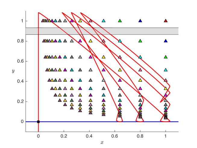
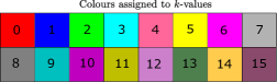
With $\mu={\bf 0}$ , (8.1) satisfies the conditions of Theorem 3.2. In particular $\Delta_{0}=2.25$ so $\Delta_{0}>0$ and $-1<c_{2,0}<1-\frac{\Delta_{0}}{2}$ . Therefore (8.1) has an asymptotically stable single-round periodic solution for all sufficiently large values of $k$ . In fact these exist for all $k\geq 1$ , see Fig. 3, plus there exists an asymptotically stable fixed point at $(x,y)=(1,1)$ that can be interpreted as corresponding to $k=0$ .

In this remainder of this section we study how the infinite coexistence is destroyed by varying each the components of $\mu$ from zero in turn. We identify saddle-node and period-doubling bifurcations numerically and compare these to our above asymptotic results. First, by varying the value of $\mu_{1}$ from zero we destroy the homoclinic tangency. Indeed in (5.5) we have ${\bf n}_{\rm tang}^{\sf T}=[1,0,0,0]$ . Thus if we fix $\mu_{2}=\mu_{3}=\mu_{4}=0$ and vary the value of $\mu_{1}$ , by Theorem 6.1 there must exist sequences of saddle-node and period-doubling bifurcations occurring at values of $\mu_{1}$ that are asymptotically proportional to $\alpha^{2k}$ . Fig. 4a shows the bifurcation values (obtained numerically) for six different values of $k$ . We have designed (8.1) so that it satisfies (7.2). Consequently the formulas (7.22) and (7.23) for the bifurcation values can be applied directly. In panel (b) we observe that the numerically computed bifurcation values indeed converge to their leading-order approximations.

We now fix $\mu_{1}=\mu_{3}=\mu_{4}=0$ and vary the value of $\mu_{2}$ . This parameter variation alters the product of the eigenvalues associated with the origin. Specifically ${\bf n}_{\rm eig}^{\sf T}=\mathopen{}\mathclose{{}\left[0,\frac{1}{\alpha},0,0}\right]$ in (4.3) so by Theorem 6.1 the bifurcation values are asymptotically proportional to $\frac{\alpha^{k}}{k}$ . In Fig. 5 we see the numerically computed bifurcation values converging to their leading order approximations (7.24) and (7.25).

Next we fix $\mu_{1}=\mu_{2}=\mu_{4}=0$ and vary the value of $\mu_{3}$ which breaks the global resonance condition. Here ${\bf n}_{\rm tang}^{\sf T}{\bf v}=0$ and ${\bf n}_{\rm eig}^{\sf T}{\bf v}=0$ so Theorem (6.1) does not apply. But by performing calculations analogous to those given above in the proof of Theorem 6.1 directly to the map (8.1), we obtain the following expressions for the saddle-node and period-doubling bifurcation values

\epsilon_{\rm SN}=\frac{(1-c_{2,0})^{2}}{4d_{5,0}}\alpha^{k}+\mathcal{O}(|\alpha|^{2k}),

(8.7)

\epsilon_{\rm PD}=-\frac{3(1-c_{2,0})^{2}}{4d_{5,0}}\alpha^{k}+\mathcal{O}(|\alpha|^{2k}).

(8.8)

Fig. 6 shows that the numerically computed bifurcations do indeed appear to be converging to the leading-order components of (8.7) and (8.8). Notice the bifurcation values are asymptotically proportional to $\alpha^{k}$ (a slightly slower rate than that in Fig. 5).

Finally we fix $\mu_{1}=\mu_{2}=\mu_{3}=0$ and vary the value of $\mu_{4}$ which breaks the condition on the resonance terms in $T_{0}$ . As in the previous case Theorem 6.1 does not apply. By again calculating the bifurcations as above we obtain

\epsilon_{{\rm SN}}=\frac{(1-c_{2,0})^{2}}{4d_{5,0}k}+\mathcal{O}\mathopen{}\mathclose{{}\left(\frac{1}{k^{2}}}\right),

(8.9)

\epsilon_{{\rm PD}}=-\frac{3(1-c_{2,0})^{2}}{4d_{5,0}k}+\mathcal{O}\mathopen{}\mathclose{{}\left(\frac{1}{k^{2}}}\right),

(8.10)

and these agree with the numerically computed bifurcation values as shown in Fig. 7. The bifurcation values are asymptotically proportional to $\frac{1}{k}$ which is substantially slower than in the previous three cases.

9 Discussion

In this paper we have considered globally resonant homoclinic tangencies in smooth two-dimensional maps and determined scaling laws for the size of parameter intervals in which single-round periodic solutions are asymptotically stable. We have illustrated the results with an abstract four-parameter family. It remains to identify globally resonant homoclinic tangencies in prototypical maps and maps derived from physical applications.

About a parameter point satisfying the conditions of Theorem 3.2, for any positive $j\in\mathbb{Z}$ there exists an open region of parameter space in which the family of maps has $j$ coexisting asymptotically stable periodic solutions. It follows from Theorem 6.1 that the largest ball (sphere) that the region contains has a diameter asymptotically proportional to $|\alpha|^{2j}$ . But, as we have shown, different directions of perturbation yield different scaling laws. Consequently we expect such regions to have an elongated shape for large values of $j$ . Indeed preliminary investigations reveal that such regions may have a particularly complicated shape, bounded by many of the saddle-node and periodic-doubling bifurcations identified above.

We believe the primary $|\alpha|^{2k}$ scaling law holds true for higher-dimensional maps. Certainly similar aspects of homoclinic tangencies have been shown to be independent of dimension, [6]. Also in the piecewise-linear setting, globally resonant homoclinic tangencies were analysed in [16].

Appendix A Proof of Lemma 7.1

Write

T_{0}(x,y)=\begin{bmatrix}\lambda x\mathopen{}\mathclose{{}\left(1+a_{1}xy+x^{2}y^{2}\tilde{F}(x,y)}\right)\\ \sigma y\mathopen{}\mathclose{{}\left(1+b_{1}xy+x^{2}y^{2}\tilde{G}(x,y)}\right)\end{bmatrix}.

(A.1)

Let $R>0$ be such that

|a_{1}|,|b_{1}|,|\tilde{F}(x,y)|,|\tilde{G}(x,y)|\leq R

(A.2)

for all $(x,y)\in\mathcal{N}$ and all sufficiently small values of $\mu$ . For simplicity we assume $\alpha>0$ ; if instead $\alpha<0$ the proof can be completed in the same fashion.

We have $\lambda=\alpha+\mathcal{O}\mathopen{}\mathclose{{}\left(|\alpha|^{k}}\right)$ and $\sigma=\frac{1}{\alpha}+\mathcal{O}\mathopen{}\mathclose{{}\left(|\alpha|^{k}}\right)$ . Thus there exists $M\geq 2R$ such that $\lambda\leq\alpha\mathopen{}\mathclose{{}\left(1+M\alpha^{k}}\right)$ and $\sigma\leq\frac{1}{\alpha}\mathopen{}\mathclose{{}\left(1+M\alpha^{k}}\right)$ for sufficiently large values of $k$ . It follows (by induction on $j$ ) that

\sigma^{j}\leq\alpha^{-j}\mathopen{}\mathclose{{}\left(1+2Mj\alpha^{k}}\right),

(A.3)

and

\mathopen{}\mathclose{{}\left(\lambda\sigma}\right)^{j}\leq 1+4Mj\alpha^{k},

(A.4)

for all $j=1,2,\ldots,k$ again assuming $k$ is sufficiently large.

Let $\varepsilon>0$ . Assume

\displaystyle|x-1|

\displaystyle\leq\varepsilon,

\displaystyle\mathopen{}\mathclose{{}\left|\alpha^{-k}y-1}\right|

\displaystyle\leq\varepsilon,

(A.5)

for sufficiently large values of $k$ . We can assume $\varepsilon<1-\frac{1}{\sqrt{2}}$ so then

\frac{\alpha^{k}}{2}\leq|xy|\leq 2\alpha^{k}.

(A.6)

Write

T_{0}^{j}(x,y)=\begin{bmatrix}\lambda^{j}x\mathopen{}\mathclose{{}\left(1+ja_{1}xy+x^{2}y^{2}\tilde{F}_{j}(x,y)}\right)\\ \sigma^{j}y\mathopen{}\mathclose{{}\left(1+jb_{1}xy+x^{2}y^{2}\tilde{G}_{j}(x,y)}\right)\end{bmatrix}.

(A.7)

Below we will use induction on $j$ to show that

\mathopen{}\mathclose{{}\left|\tilde{F}_{j}(x,y)}\right|,\mathopen{}\mathclose{{}\left|\tilde{G}_{j}(x,y)}\right|\leq 12Mj^{2},

(A.8)

for all $j=1,2,\ldots,k$ , assuming $k$ is sufficiently large. This will complete the proof because with $j=k$ , (A.8) implies (7.1).

Clearly (A.8) is true for $j=1$ : $\mathopen{}\mathclose{{}\left|\tilde{F}_{1}(x,y)}\right|=\mathopen{}\mathclose{{}\left|\tilde{F}(x,y)}\right|\leq R\leq\frac{M}{2}<12M$ and similarly for $\tilde{G}_{1}$ . Suppose (A.8) is true for some $j<k$ . It remains for us to verify (A.8) for $j+1$ . First observe that by using $|a_{1}|\leq R$ , (A.6), and the induction hypothesis,

\mathopen{}\mathclose{{}\left|1+ja_{1}xy+x^{2}y^{2}\tilde{F}_{j}(x,y)}\right|\leq 1+2Rj\alpha^{k}+48Mj^{2}\alpha{2k}.

For sufficiently large $k$ this implies

\mathopen{}\mathclose{{}\left|1+ja_{1}xy+x^{2}y^{2}\tilde{F}_{j}(x,y)}\right|\leq 1+2Mj\alpha^{k},

(A.9)

where we have also used $M\geq 2R$ . Similarly

\mathopen{}\mathclose{{}\left|1+jb_{1}xy+x^{2}y^{2}\tilde{G}_{j}(x,y)}\right|\leq 1+2Mj\alpha^{k}.

(A.10)

Write $T_{0}^{j}(x,y)=(x_{j},y_{j})$ . By using (A.3), (A.5), and (A.10) we obtain

|y_{j}|\leq\alpha^{k-j}(1+\varepsilon)\mathopen{}\mathclose{{}\left(1+2Mj\alpha^{k}}\right)^{2}.

Thus $|y_{j}|\leq\alpha^{k-j}(1+2\varepsilon)$ , say, for sufficiently large values of $k$ . Also $|x_{j}y_{j}|$ is clearly small, so we can conclude that $(x_{j},y_{j})\in\mathcal{N}$ (in particular we have shown that $(x_{k-1},y_{k-1})$ can be made as close to $\mathopen{}\mathclose{{}\left(0,\frac{1}{\alpha}}\right)$ as we like).

By matching the first components of $T_{0}^{j+1}(x,y)=\mathopen{}\mathclose{{}\left(T_{0}\circ T_{0}^{j}}\right)(x,y)$ we obtain

	$\displaystyle\lambda^{j+1}x\mathopen{}\mathclose{{}\left(1+(j+1)a_{1}xy+x^{2}y^{2}\tilde{F}_{j+1}(x,y)}\right)$	$\displaystyle=\lambda^{j+1}x\mathopen{}\mathclose{{}\left(1+ja_{1}xy+x^{2}y^{2}\tilde{F}_{j}(x,y)}\right)$
		$\displaystyle\quad+\lambda^{j+1}a_{1}x^{2}y(1+P)+\lambda^{j+1}x^{3}y^{2}Q,$		(A.11)

where

	$\displaystyle 1+P$	$\displaystyle=\mathopen{}\mathclose{{}\left(\lambda\sigma}\right)^{j}\mathopen{}\mathclose{{}\left(1+ja_{1}xy+x^{2}y^{2}\tilde{F}_{j}(x,y)}\right)^{2}\mathopen{}\mathclose{{}\left(1+jb_{1}xy+x^{2}y^{2}\tilde{G}_{j}(x,y)}\right),$		(A.12)
	$\displaystyle Q$	$\displaystyle=\mathopen{}\mathclose{{}\left(\lambda\sigma}\right)^{2j}\mathopen{}\mathclose{{}\left(1+ja_{1}xy+x^{2}y^{2}\tilde{F}_{j}(x,y)}\right)^{3}\mathopen{}\mathclose{{}\left(1+jb_{1}xy+x^{2}y^{2}\tilde{G}_{j}(x,y)}\right)^{2}\tilde{F}(x_{j},y_{j}).$		(A.13)

By (A.4), (A.9), and (A.10), we obtain

	$\displaystyle 1+P$	$\displaystyle\leq\mathopen{}\mathclose{{}\left(1+4Mj\alpha^{k}}\right)\mathopen{}\mathclose{{}\left(1+2Mj\alpha^{k}}\right)^{3}$
		$\displaystyle\leq 1+11Mj\alpha^{k},$
	$\displaystyle Q$	$\displaystyle\leq\mathopen{}\mathclose{{}\left(1+4Mj\alpha^{k}}\right)^{2}\mathopen{}\mathclose{{}\left(1+2Mj\alpha^{k}}\right)^{5}R$
		$\displaystyle\leq 2R,$

assuming $k$ is sufficiently large and where we have also used $|\tilde{F}(x_{j},y_{j})|\leq R$ (valid because $(x_{j},y_{j})\in\mathcal{N}$ ). From (A.11),

\tilde{F}_{j+1}(x,y)=\tilde{F}_{j}(x,y)+\frac{P}{xy}+Q.

Then by using the induction hypothesis, the lower bound on $|xy|$ (A.6), and the above bounds on $P$ and $Q$ , we arrive at

	$\displaystyle\mathopen{}\mathclose{{}\left\|\tilde{F}_{j+1}(x,y)}\right\|$	$\displaystyle\leq 12Mj^{2}+22Mj+2R$
		$\displaystyle\leq 12Mj^{2}+24Mj$
		$\displaystyle<12M(j+1)^{2}.$

In a similar fashion by matching the second components of $T_{0}^{j+1}(x,y)=\mathopen{}\mathclose{{}\left(T_{0}\circ T_{0}^{j}}\right)(x,y)$ we obtain $\mathopen{}\mathclose{{}\left|\tilde{G}_{j+1}(x,y)}\right|<12M(j+1)^{2}$ . This verifies (A.8) for $j+1$ and so completes the proof. $\Box$

References

[1] A. Delshams, M. Gonchenko, and S. Gonchenko. On dynamics and bifurcations of area preserving maps with homoclinic tangencies. Nonlinearity, 28:3027–3071, 2015.
[2] Y. Do and Y. C. Lai. Multistability and arithmetically period-adding bifurcations in piecewise smooth dynamical systems. Chaos, 18(4):043107, 2008.
[3] N.K. Gavrilov and L.P. Silnikov. On three dimensional dynamical systems close to systems with structurally unstable homoclinic curve. I. Math. USSR Sbornik, 17:467–485, 1972.
[4] N.K. Gavrilov and L.P. Silnikov. On three-dimensional dynamical systems close to systems with a structurally unstable homoclinic curve. II. Math. USSR Sbornik, 19:139–156, 1973.
[5] M.S. Gonchenko and S.V. Gonchenko. On cascades of elliptic periodic points in two-dimensional symplectic maps with homoclinic tangencies. Regul. Chaotic Dyns., 14:116–136, 2009.
[6] S. V. Gonchenko, L. P. Shil’nikov, and D. V. Turaev. Quasiattractors and homoclinic tangencies. Comput. Math. Appl., 34(2–4):195–227, 1997.
[7] S.V. Gonchenko and L.P. Shilnikov. On two-dimensional area-preserving maps with homoclinic tangencies that have infinitely many generic elliptic periodic points. J. Math. Sci. (N. Y.), 128:2767–2773, 2005.
[8] V.S. Gonchenko, Yu.A. Kuznetsov, and H.G.E. Meijer. Generalized Hénon map and bifurcations of homoclinic tangencies. SIAM J. Appl. Dyn. Syst., 2005.
[9] Y. A. Kuznetsov and H. G. E. Meijer. Numerical Bifurcation Analysis of Maps: From Theory to Software. Cambridge Monographs on Applied and Computational Mathematics. Cambridge University press, 2019.
[10] S.S. Muni, R.I. McLachlan, and D.J.W. Simpson. Homoclinic tangencies with infinitely many asymptotically stable single-round periodic solutions. Discrete Contin Dyn Syst Ser A, 2021.
[11] S.E. Newhouse. Diffeomorphisms with infinitely many sinks. Topology, 13:9–18, 1974.
[12] J. Palis and F. Takens. Hyperbolicity and sensitive chaotic dynamics at homoclinic bifurcations. Cambridge University Press, New York, 1993.
[13] L. P. Shilnikov, A. L. Shilnikov, D. V. Turaev, and L. O. Chua. Methods of Qualitative Theory in Nonlinear Dynamics. World Scientific, 1998.
[14] D.J.W. Simpson. Scaling laws for large numbers of coexisting attracting periodic solutions in the border-collision normal form. Int. J. Bifurcation Chaos, 24:1450118, 2014.
[15] D.J.W. Simpson. Sequences of periodic solutions and infinitely many coexisting attractors in the border-collision normal form. Int. J. Bifurcation Chaos, 24:1430018, 2014.
[16] D.J.W. Simpson and C.P. Tuffley. Subsumed homoclinic connections and infinitely many coexisting attractors in piecewise-linear continuous maps. Int. J. Bifurcation Chaos, 27, 2017.
[17] S. Sternberg. On the structure of local homeomorphisms of Euclidean $n$ -space, II. Amer. J. Math., 1958.