Underwater Image Quality Assessment: A Perceptual Framework Guided by Physical Imaging
Abstract
In this paper, we propose a physically imaging-guided framework for underwater image quality assessment (UIQA), called PIGUIQA. First, we formulate UIQA as a comprehensive problem that considers the combined effects of direct transmission attenuation and backwards scattering on image perception. On this basis, we incorporate advanced physics-based underwater imaging estimation into our method and define distortion metrics that measure the impact of direct transmission attenuation and backwards scattering on image quality. Second, acknowledging the significant content differences across various regions of an image and the varying perceptual sensitivity to distortions in these regions, we design a local perceptual module on the basis of the neighborhood attention mechanism. This module effectively captures subtle features in images, thereby enhancing the adaptive perception of distortions on the basis of local information. Finally, by employing a global perceptual module to further integrate the original image content with underwater image distortion information, the proposed model can accurately predict the image quality score. Comprehensive experiments demonstrate that PIGUIQA achieves state-of-the-art performance in underwater image quality prediction and exhibits strong generalizability. The code for PIGUIQA is available on https:// anonymous.4open.science/r/PIGUIQA-A465/.
1 Introduction
The underwater world is rich in resources, and underwater images provide a crucial medium for exploring environments such as oceans and lakes by accurately and intuitively capturing underwater information. However, the complexities of the underwater imaging environment often result in suboptimal image quality [14, 47]. Therefore, underwater image quality assessment (UIQA) is fundamental for underwater image processing. UIQA methods help determine whether underwater images meet quality requirements for various applications and assess the visual quality of enhanced underwater images.
According to the accessibility of ideal references, image quality assessment (IQA) methods can be broadly categorized into full-reference (FR) and no-reference (NR) approaches. For underwater images, obtaining perfect undistorted references is often impractical; thus, typical FR-IQA approaches, such as the structural similarity index measure (SSIM) [36] and feature similarity indexing method (FSIM) [43], are not applicable. Although NR-IQA approaches [26, 7, 29] have been developed for many years, most of them are designed to evaluate generic images. Many NR-IQA methods [21, 28, 19] are based on statistical properties, such as natural scene statistics (NSS), which are typically observed under good lighting conditions and in clear visual environments. However, the unique characteristics of underwater environments result in light propagation and scattering rules that are significantly different from those in terrestrial natural scenes. As a result, the statistical properties of NSSs often fall short in accurately describing and assessing the quality of underwater images.
To date, effective, robust, and widely accepted UIQA methods in the field of underwater image processing are lacking. Although several well-known UIQA methods have been developed, such as underwater color image quality evaluation (UCIQE) [41] and the underwater image quality measure (UIQM) [31], most UIQA methods are based on manual-crafted features, which often fail to fully capture the complexity and diversity of underwater imagery. In addition, these methods often prioritize images with higher color saturation, resulting in quality assessments that may not align with human visual perception. In addition to manually designed features, recent advancements in deep learning have demonstrated significant feature learning capabilities. However, only a few studies [16] have applied deep learning to UIQA. This is because deep learning models typically require large amounts of labelled data for training, but the existing annotated underwater image datasets are relatively small. The data dependency in deep learning also makes ensuring the generalization capability of deep learning models challenging.

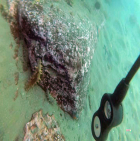
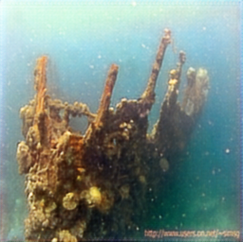
Another primary challenge is that underwater images differ markedly from terrestrial images because of their specific imaging environments and lighting conditions. As a result, traditional NR-IQA methods that perform well in terrestrial image processing cannot be directly applied to underwater images. Specifically, as shown in Fig. 1, the underwater environment is complex and variable, with light propagation affected by scattering and absorption. Different wavelengths of light attenuate at different rates, with longer wavelengths diminishing more rapidly in water. Consequently, shorter wavelengths such as green and blue light can travel further underwater, causing underwater images to exhibit a blue–green hue and suffering from significant color distortion. The scattering of light in water can be categorized into forward scattering and backwards scattering on the basis of the angle. Forward scattering occurs when light reflected from the target object deviates from its original path before it reaches the sensor, resulting in blurred underwater images. Backwards scattering, on the other hand, involves a large amount of stray light entering the sensor, leading to visual issues such as loss of detail, low overall contrast, and increased background noise in underwater images. The need for the development of specialized UIQA methods that can effectively address the unique challenges posed by underwater imaging is urgent.
To address the aforementioned issues, combining prior knowledge of underwater imaging with the excellent feature extraction capabilities of deep learning presents an effective solution. On this basis, we propose a physically imaging-guided framework for UIQA (PIGUIQA) by integrating the physical model of underwater light propagation with deep learning techniques. Specifically, the framework considers distortions caused by backwards scattering and direct transmission processes. These factors play crucial roles in underwater imaging, influencing image clarity, contrast, and color representation. Within the PIGUIQA framework, we leverage the powerful feature extraction capabilities of deep learning models to capture both local details and global perceptual features in images. Capturing local details allows the model to perceive distortions in critical regions of underwater images, such as object edges and texture information, whereas global perceptual features help the model understand the overall structure and context of the entire image. The main contributions of this work can be summarized as follows:
-
•
We formulate UIQA as a comprehensive problem that accounts for the combined effects of direct transmission attenuation and backwards scattering on image perception. We integrate advanced physics-based underwater imaging estimations into our framework. From the perspective of matrix theory, we define distortion metrics to measure these impacts.
-
•
We design a neighborhood attention (NA)-based local perceptual module to capture subtle features in images, thereby enhancing the adaptive perception of distortions via local information. Additionally, a global perceptual module is employed to integrate the original image content with underwater image distortion information, assisting the model in understanding the overall structure and context of the entire image.
-
•
The experimental results demonstrate that the proposed method effectively evaluates underwater image quality, achieving superior performance across various correlation coefficients and error metrics. Furthermore, a cross-dataset experiment also confirms the strong generalizability and robustness of the proposed method.
2 Related Work
Owing to the unique characteristics of underwater images, conventional NR-IQA methods [26, 27, 44, 34] are not suitable for evaluating underwater images. Consequently, researchers have begun to focus on specially designed UIQA methods, and many important studies have emerged in this field. Yang et al. [41] proposed the underwater color image quality evaluation method (UCIQE), which quantifies quality attributes such as color bias, blurriness, and contrast through a linear combination of chromaticity, saturation, and contrast measurements. Panetta et al. [31] introduced an underwater image quality measure (UIQM) from the perspective of the human visual system (HVS), which considers colorfulness, sharpness, and contrast, thereby addressing some limitations of the UCIQE. Guo et al. [9] also focused on these three features and conducted experiments on a self-constructed small-scale dataset containing only 200 underwater enhanced images, which may restrict its performance on larger datasets. Wang et al. [35] developed a UIQA method called the CCF that incorporates factors such as colorfulness, contrast, and fog density. Yang et al. [42] introduced a frequency domain UIQA metric (FDUM), which, like UIQM, considers colorfulness, contrast, and sharpness but analyses these features in the frequency domain and integrates the dark channel prior (DCP) [11]. Jiang et al. [15] proposed a no-reference underwater image quality (NUIQ) metric that transforms underwater images from the RGB space to the opponent color space (OC); extracts color, luminance, and structural features in the OC space; and employs support vector machines (SVMs) for quality assessment. Zheng et al. [48] introduced the underwater image fidelity (UIF) metric, which evaluates the naturalness, sharpness, and structural indicators in the CIELab color space. Guo et al. [10] presented an underwater image enhancement quality metric (UWEQM) that considers features such as transmission medium maps, Michaelson-like contrast, salient local binary patterns, and simplified color autocorrelograms. Liu et al. [23] developed an underwater image quality index (UIQI) by extracting features related to luminance, color cast, sharpness, contrast, fog density, and noise, using support vector regression (SVR) to predict image quality. However, these methods, which rely on handcrafted features and regression techniques, still have limitations, as they do not comprehensively characterize image quality and may not be effective for various types of underwater images.
With the rapid advancement of deep neural networks, there is an urgent need for end-to-end UIQA methods that can automatically learn useful features from data and predict image quality more accurately. Fu et al. [4] proposed a rank learning framework, which was the first to utilize deep learning for UIQA. This method generates a set of medium-quality images by blending original images with their corresponding reference images at varying degrees and employs a Siamese network to learn their quality rankings. Wang et al. [37] introduced a generation-based joint luminance-chrominance underwater image quality evaluation (GLCQE) method. GLCQE first employs DenseUNet to generate two reference images—one unenhanced and one optimally enhanced—and uses these images to assess chromatic and luminance distortions while also designing a parallel spatial attention module to represent image sharpness. Recognizing that deep learning often requires large datasets for training, Jiang et al. [16] constructed a dataset for UIQA with multidimensional quality annotations and proposed a multistream collaborative learning network (MCOLE). This method trains three specialized networks to extract color, visibility, and semantic features, facilitating quality prediction through multistream collaborative learning.
Despite the significant progress made by these deep learning methods in UIQA, they often lack consideration of the underwater imaging process and may only be effective on specific datasets, limiting their generalization capabilities. Therefore, integrating prior knowledge of the underwater imaging process with deep learning techniques is an effective strategy for addressing these challenges.
3 Methodology
3.1 Problem formulation

The problem of IQA can be formulated as the task of finding a function that produces evaluation results closely aligned with the true quality of an image. This can be expressed mathematically as follows:
| (1) |
where represents the ground truth quality of an image , typically expressed in terms of the mean opinion score (MOS). denotes the mathematical expectation. This problem involves identifying a function capable of accurately reflecting various image attributes, such as sharpness, contrast, color, and noise levels, to derive an accurate quality score.
For underwater images, we specifically analyse image quality by considering the causes of distortion inherent to underwater imaging. In real underwater scenarios, the camera is often positioned close to the underwater scene. Consequently, the impact of forward scattering on image quality can be neglected, resulting in only direct transmission attenuation and backwards scattering components to be considered. This relationship is represented as:
| (2) |
where represents the perfect image, represents the corresponding distorted image, denotes the transmission attenuation matrix, and denotes the background clutter matrix. The symbol denotes the Hadamard product.
Both and can be estimated via traditional modelling methods that are based on prior knowledge [2] or by employing deep learning models trained on synthetic underwater image datasets [38]. The all-ones matrix is denoted as , and the zero matrix is denoted as . For a high-quality image, the direct transmission attenuation matrix should be “closer” to , whereas the background noise matrix should be “closer” to . Thus, we introduce the concept of imaging-perceived distortion, which is directly correlated with the distances between and and between and . Given that perceived distortion is closely related to the image content itself, the UIQA problem can be formulated as follows:
| (3) |
where is the ground-truth quality of an underwater image and where and represent the distance maps measuring transmission attenuation and backwards scattering distortion between and and between and , respectively. and are local distortion-aware functions to be learned, and is a global perceptual function to be learned. This formulation captures the essential aspects of UIQA by integrating a physical model into the evaluation process.
3.2 Framework
Fig. 2 illustrates the proposed framework for UIQA. The process begins with an underwater image, which is processed through an image estimation module that generates two key maps: the transmission attenuation map and the background clutter map . Transmission attenuation and background clutter distortions are quantified by evaluating the distance between each patch of and an all-one matrix and the distance between each patch of and a zero matrix, respectively. These distortions are denoted as and . The local perceptual modules and subsequently capture local scattering and transmission distortion characteristics. After local processing, the outputs of these modules are scaled by and and then fused with the original image. This combined data is then passed through a global perceptual network , which integrates the information from all previous stages to generate a final prediction. The proposed framework effectively combines local distortion correction with global perceptual adjustment, which is tailored specifically for underwater optical scenarios.
3.3 Underwater Imaging Estimation
A commonly used precise revised underwater image formation model [1] is as follows:
| (4) | ||||
where is the color channel; and are distortion-free and distorted images, respectively; is the object‒camera distance; is the background ambient light image; and and are the direct attenuation and backwards scattering coefficients, respectively.
In this paper, we utilize the SyreaNet model proposed by Wen et al. [38] for underwater imaging estimation, which is represented mathematically as follows:
| (5) |
This method synthesizes more formal underwater images under various conditions via the imaging model described in Eq. (4). Subsequently, it trains on the synthesized underwater image data to estimate the transmission attenuation matrix and background clutter matrix , as defined in Eq. (2). Compared with traditional manual estimation of underwater imaging parameters, which often lacks accuracy, SyreaNet integrates physical modelling with the interpretability of imaging models and the feature extraction capabilities of neural networks. As illustrated in Fig. 3, it can automatically learn and extract features, adaptively incorporating prior knowledge on the basis of different underwater environments and imaging conditions. This results in improved adaptability and robustness in underwater imaging estimation.


(a)

(b)

(c)

(d)
3.4 Imaging Distortion Measurements
Considering the varying depths and optical properties of different regions and objects in underwater images, we decompose the image transmission attenuation map and the background clutter map into patches of size . This strategy facilitates the model’s learning of local features, thereby enhancing the perception of details in images with intricate content. Consequently, we address the design of imaging distortion metrics for each patch.
For the transmission attenuation map , which ideally should resemble the all-ones matrix , we define a linear operator for any matrix as follows:
| (6) |
where is the -th patch of . On the basis of this definition, we establish the transmission attenuation distortion metric for a patch of size as the norm of the linear transformation :
| (7) |
According to the functional analysis theory, we have:
| (8) |
where denotes the largest eigenvalue of the operator. Since
| (9) |
where is the -th element of and where is an matrix with the -th element as 1 and all other elements as 0, serves as the eigenvalue of . Therefore, we define the transmission attenuation distortion measurement in the -th patch as follows:
| (10) |
The background clutter map can be regarded as an additional noise overlay on the original image, arising from background textures, variations in lighting, or the presence of nontarget objects. According to the theory of human visual sensitivity, the HVS can only distinctly recognize distortion when the intensity of the noise surpasses a specific perceptual threshold. Thus, we propose a backwards scattering distortion measurement for the -th patch of :
| (11) |
where is the -th element of . The core idea of this measurement is that for each local patch, the degree of distortion can be quantified by the maximum noise value within that region, as the peak noise level typically generates the most significant visual interference, making it more readily detectable by the HVS. At this point, we can obtain and via Eq. (3).
3.5 Perceptual Networks
High-quality underwater images typically exhibit good contrast, smooth and consistent textures, and sharp edges in local regions. Therefore, analysing the correlation between each pixel and its neighbouring pixels is essential. Compared with traditional self-attention and convolutional methods, the NA mechanism effectively captures local textures and details, providing higher fidelity in processing local information. This enhanced precision in detecting subtle quality differences makes it especially suitable for the IQA task. Accordingly, we developed a local perceptual module based on the NA mechanism.
Let , , and denote the -dimensional query, key, and value vectors of the -th input, respectively, obtained through linear projection. The neighborhood of size for the -th input is defined as , where represents the -th nearest neighbor to . The neighbourhood attention operation on is given by:
| (12) |
where is the key matrix, is the value matrix, and is the relative positional bias matrix. denotes the transpose of matrix .
Therefore, as illustrated in Fig. 4, we define the local distortion-aware functions and in equation (3) as two distinct residual NA transformer blocks (RNATB):
| (13) | |||
| (14) |

In addition to perceiving local detail distortions, the model must also capture global perceptual features. This capability helps the model understand the overall structure and context of the image. For efficient extraction of global features, we utilize the architecture of the classical CNN model ResNet50 [12], with modifications to the input channel count. Consequently, we define the global perceptual function in Eq. (3) as follows:
| (15) | ||||
where denotes the concatenation operation and where represents the predicted image quality score. This dual approach to feature extraction, encompassing both local and global perspectives, enhances the comprehensiveness and precision of the assessment process, thereby improving the accuracy of the UIQA.
Finally, the optimization of Eq. (3) is equivalent to minimizing the following loss function:
| (16) |
where denotes the L2 norm.
4 Experiments
4.1 Experimental Settings
| SAUD2.0 (80%) SAUD2.0 (20%) | SAUD2.0 (100%) UID2021 (100%) | |||||||
| IQA Method | PLCC | SRCC | KRCC | RMSE | PLCC | SRCC | KRCC | RMSE |
| BRISQUE [26] | 0.5276 | 0.5018 | 0.3533 | 17.9813 | 0.3248 | 0.3097 | 0.2088 | 2.0384 |
| BLIINDSII [32] | 0.4816 | 0.4449 | 0.3060 | 19.4931 | 0.1635 | 0.1701 | 0.1145 | 2.1262 |
| BIQME [8] | 0.4938 | 0.4553 | 0.3168 | 17.6922 | 0.4274 | 0.3652 | 0.2484 | 1.9485 |
| FRIQUEE [5] | 0.7882 | 0.7738 | 0.5843 | 13.1197 | 0.3150 | 0.3042 | 0.2053 | 2.0455 |
| NRSL [19] | 0.5176 | 0.4904 | 0.3382 | 18.2603 | 0.2887 | -0.2781 | -0.1867 | 2.0634 |
| RISE [18] | 0.1310 | 0.1037 | 0.0713 | 21.0194 | 0.2760 | 0.2647 | 0.1749 | 2.0715 |
| DIIVINE [28] | 0.5151 | 0.5016 | 0.3523 | 18.2658 | 0.1214 | 0.1199 | 0.0798 | 2.1393 |
| DBCNN [45] | 0.7744 | 0.7633 | 0.5704 | 14.6094 | 0.3840 | 0.3794 | 0.2564 | 1.9589 |
| WaDIQaM [3] | 0.8408 | |||||||
| B-FEN [39] | 0.8512 | 0.6595 | 10.8642 | 0.4841 | 0.4766 | 0.3261 | 1.8564 | |
| UCIQE [40] | 0.3674 | 0.3719 | 0.2597 | 19.9196 | 0.3238 | 0.3080 | 0.2080 | 2.0391 |
| UIQM [30] | 0.3498 | 0.2902 | 0.1993 | 19.9120 | 0.2480 | 0.1395 | 0.0926 | 2.0879 |
| CCF [35] | 0.1664 | 0.1624 | 0.1088 | 20.9302 | 0.3204 | 0.1759 | 0.1164 | 2.0416 |
| FDUM [42] | 0.2815 | 0.2613 | 0.1785 | 20.1235 | 0.3229 | 0.3364 | 0.2307 | 2.0397 |
| NUIQ [15] | 0.7413 | 0.7480 | 0.5471 | 14.1152 | 0.3143 | 0.3134 | 0.2078 | 2.0460 |
| MCOLE [16] | ||||||||
| PIGUIQA (ours) | ||||||||
-
•
“A () B ()” means training on the data of dataset “A” and testing on the data of dataset “B”. The general-purpose methods and the specific-purpose methods are separated by a horizontal line. In each column, the three best values are bolded in red (1st), green (2nd), and blue (3rd) colors, respectively. Some of the data in the table are obtained from the literature.

(a) Train and test on SAUD2.0

(b) Train and test on UID2021

(c) Train and test on UWIQA

(d) Train on SAUD2.0 and test on UID2021
| IQA Method | PLCC | SRCC | KRCC | RMSE |
|---|---|---|---|---|
| BRISQUE [26] | 0.6439 | 0.6343 | 0.4623 | 1.6407 |
| BLIINDSII [32] | 0.5451 | 0.5216 | 0.3688 | 1.7934 |
| NIQE [27] | 0.3384 | 0.3304 | 0.2219 | 2.0464 |
| IL-NIQE [44] | 0.4644 | 0.4630 | 0.4321 | 1.9121 |
| NRSL [19] | 0.6643 | 0.6504 | 0.4655 | 1.6016 |
| RISE [18] | 0.6219 | 0.6034 | 0.4314 | 1.6812 |
| DIIVINE [28] | 0.6264 | 0.6112 | 0.4363 | 1.6716 |
| DBCNN [45] | 0.7594 | 0.7535 | 0.5523 | 1.3862 |
| WaDIQaM [3] | 0.7659 | |||
| B-FEN [39] | 0.7713 | 0.5732 | 1.3696 | |
| UCIQE [40] | 0.6474 | 0.6150 | 0.4503 | 1.6335 |
| UIQM [30] | 0.4760 | 0.4613 | 0.3192 | 1.8769 |
| CCF [35] | 0.5208 | 0.4236 | 0.2990 | 1.8351 |
| FDUM [42] | 0.6092 | 0.5823 | 0.4189 | 1.7057 |
| NUIQ [15] | 0.7266 | 0.7168 | 0.5293 | 1.4762 |
| MCOLE [16] | ||||
| PIGUIQA (ours) |
-
•
The general-purpose methods and the specific-purpose methods are separated by a horizontal line. In each column, the three best values are bolded in red (1st), green (2nd), and blue (3rd) colors, respectively. Some of the data in the table are obtained from the literature.
Databases. The experiments are conducted on three databases: SAUD2.0 (2024) [16], UID2021 (2023) [13], and UWIQA (2021) [23]. The images in these datasets are sourced from real-world scenarios, and their subjective scores are MOSs, which are obtained through the single-stimulus absolute category rating (SS-ACR) methodology. Specifically, SAUD2.0 comprises 2,600 images (200 raw and 2,400 enhanced), UID2021 consists of 1,060 images (60 raw and 1,000 enhanced), and UWIQA includes 890 raw images.
Implementation details. The proposed FIGUIQA network is trained ***The implementation code is programmed in PyTorch and is publicly available at https://anonymous.4open.science/r/PIGUIQA-A465/. The experiments are run on a PC with a Linux operating system and are configured with an NVIDIA GeForce RTX 4090 GPU with 24 GB of memory. using the default settings of the Adam optimizer. The learning rate is set to . To ensure the stability of the final model, a total of 1000 epochs are conducted during training. To prevent overfitting, data augmentation techniques such as random horizontal and vertical flipping, as well as rotation within the range of degrees, are employed. The size of patches is set to , which is a common setting in computer vision.
Evaluation criteria. To validate the effectiveness and performance of the proposed UIQA method, we employ four commonly used evaluation metrics: the Pearson linear correlation coefficient (PLCC), the Spearman rank correlation coefficient (SRCC), the Kendall rank correlation coefficient (KRCC), and the root mean square error (RMSE). In accordance with standard practice, we apply nonlinear five-parameter logistic regression (5PL) to fit the relationship between the predicted scores and the MOS prior to calculating the PLCC and RMSE.
4.2 Performance Comparison
We compare the proposed method against several commonly used no-reference image quality assessment (NR-IQA) techniques and state-of-the-art user-in-the-loop image quality assessment (UIQA) methods, including BRISQUE [26], BLIINDSII [32], NFERM [7], NIQE [27], IL-NIQE [44], SNP-NIQE [22], BIQME [8], FRIQUEE [5], PIQE [29], NRSL [19], RISE [18], DIIVINE [28], NPQI [21], dipIQ [24], HyperIQA [33], WaDIQaM, UNIQUE [46], DBCNN [45], B-FEN [39], UCIQE [40], UIQM [30], CCF [35], FDUM [42], NUIQ [15], MCOLE [16], Twice-Mix [4], and UIQI [23]. To ensure the reliability and stability of the proposed NAFRAD method, we repeat the training and testing process 10 times, using the average of the test results as the final metric.
4.2.1 Single-Dataset Scenarios
In the experimental scenario involving single datasets, we randomly selected 80% of the data from each dataset for training and used the remaining 20% for evaluation. The experimental results are presented in Tables 1, 2, and LABEL:tab:performance3. Our proposed method achieves the highest performance on the SAUD2.0 dataset, significantly surpassing the second-place method, MCOLE [16], demonstrating substantial performance improvement. Specifically, our image quality assessment method ranked first on the SAUD2.0 dataset and nearly achieved first place on the SUID2021 dataset, with only a slight margin separating it from the top performance. For the UWIQA dataset, our method ranks second. Overall, there is a noticeable trend of performance improvement as the dataset size increases, moving from UWIQA to SUID2021 and then to SAUD2.0. This trend in performance enhancement is closely related to the dataset size, which is attributable to the use of deep learning techniques in our proposed method. The effectiveness of deep learning models is typically influenced by the availability of large quantities of high-quality data.
Fig. 5 shows scatter plots of the testing dataset. This figure clearly shows that the quality scores predicted by the proposed PIGUIQA model are highly correlated with the actual MOS, with relatively small prediction errors. This indicates that our method achieves a high level of accuracy in quality score prediction. A closer examination of Fig. 5(c) reveals some unique characteristics of the UWIQA dataset. UWIQA is relatively small and has low quantization precision in its MOS labels, which are broadly categorized into only ten levels. This low-precision labelling poses challenges for training deep learning models, resulting in less effective learning of subtle image quality differences compared with other datasets.
4.2.2 Cross-Dataset Scenarios
To evaluate the generalizability of the proposed PIGUIQA method, we conducted cross-dataset experiments on the SAUD2.0 and UID2021 datasets. In this experiment, we initially trained the model on the SAUD2.0 dataset and subsequently applied the trained model to the UID2021 dataset for testing. The experimental results, presented in Table 1 and Fig. 5(d), demonstrate that our method exhibits exceptional performance under cross-dataset conditions, further validating its robustness and strong generalization ability across different datasets.
The remarkable performance in cross-dataset evaluations can be attributed to our method’s careful incorporation of prior knowledge related to underwater imaging models during the design process. The characteristics of underwater images are influenced by various factors, such as water turbidity, lighting conditions, and image distortion, resulting in significant domain specificity. To effectively address these characteristics, our approach integrates physical prior knowledge of the underwater imaging process into the modelling framework. This allows the model to adapt successfully to various types of underwater images, even when faced with different datasets.
4.3 Ablation Experiments
To validate the effectiveness of each module in the PIGUIQA method, we conducted ablation experiments on the SAUD2.0 dataset. In this experiment, we established two variables: the perception of transmission attenuation distortion and the consideration of backscattering distortion. The results, as shown in Table 4, indicate that when we remove one of the modules (i.e., retain only one distortion perception module), the model’s performance slightly decreases. This suggests that while each module independently contributes to the model’s ability to perceive certain aspects of image quality, they are not entirely independent and exhibit some interdependence. However, when both modules are removed simultaneously, there is a significant drop in the model’s performance, particularly in terms of accuracy and robustness in image quality assessment. This finding underscores the critical role that transmission attenuation distortion and backscattering distortion play as key factors in the underwater imaging process, significantly impacting the evaluation of image quality.
| IQA Method | PLCC | SRCC | KRCC | RMSE |
|---|---|---|---|---|
| BRISQUE [26] | 0.3669 | 0.3456 | 0.2562 | 0.1415 |
| NFERM [7] | 0.3925 | 0.3486 | 0.2595 | 0.1398 |
| NIQE [27] | 0.4687 | 0.4347 | 0.3243 | 0.1343 |
| IL-NIQE [44] | 0.4421 | 0.4686 | 0.3476 | 0.1364 |
| SNP-NIQE [22] | 0.5897 | 0.5516 | 0.4199 | 0.1228 |
| PIQE [29] | 0.3224 | 0.2084 | 0.1492 | 0.1441 |
| NPQI [21] | 0.6361 | 0.6078 | 0.4667 | 0.1173 |
| dipIQ [24] | 0.1369 | 0.0869 | 0.0641 | 0.1506 |
| HyperIQA [33] | 0.6501 | 0.5040 | ||
| UNIQUE [46] | 0.2386 | 0.2496 | 0.1835 | 0.1476 |
| UCIQE [40] | 0.6261 | 0.6271 | 0.4863 | 0.1185 |
| UIQM [30] | 0.5928 | 0.5960 | 0.4563 | 0.1225 |
| CCF [35] | 0.4634 | 0.4456 | 0.3344 | 0.1348 |
| FDUM [42] | 0.6462 | 0.1160 | ||
| Twice-Mix [4] | 0.4422 | 0.4727 | 0.3501 | 0.1289 |
| UIQI [23] | ||||
| PIGUIQA (ours) |
-
•
The general-purpose methods and the specific-purpose methods are separated by a horizontal line. In each column, the three best values are bolded in red (1st), green (2nd), and blue (3rd) colors, respectively. Some of the data in the table are obtained from the literature.
| Components | PLCC | SRCC | KRCC | RMSE |
|---|---|---|---|---|
| w/ | 0.9142 | 0.9043 | 0.7333 | 8.9984 |
| w/o | 0.8840 | 0.8792 | 0.6961 | 10.37 |
| w/o | 0.8738 | 0.8608 | 0.6862 | 11.19 |
| w/o | 0.8256 | 0.8320 | 0.6252 | 13.35 |
5 Conclusion
In this paper, we propose a novel physically imaging-guided framework for UIQA (PIGUIQA). By considering both direct transmission attenuation and backwards scattering effects, we integrate physical prior knowledge of the underwater imaging process into the deep learning-based model. The incorporation of advanced physics-based estimation allows for the definition of distortion metrics that capture the impact of these phenomena on visual perception. Moreover, we propose local perceptual modules based on the NA mechanism, which enhances the model’s ability to capture subtle image features and adaptively assess distortions in a region-specific manner. The experimental results demonstrate that the PIGUIQA not only outperforms existing methods in UIQA but also exhibits robust generalizability.
Supplementary Material
6 Visualization of Correlation Performance

(a) MOS:34.97

(b) MOS:37.06

(c) MOS:45.75

(d) MOS:56.03

(e) MOS:59.59

(f) MOS:38.15

(g) MOS:38.28
(h) MOS:51.24

(i) MOS:56.89

(j) MOS:65.01

(k) MOS:34.97

(l) MOS:37.06

(m) MOS:45.75
(n) MOS:56.03

(o) MOS:59.59

(p) predictions of (a)-(e)

(q) predictions of (f)-(j)

(r) predictions of (k)-(o)
This study proposes a physically imaging-guided framework for underwater image quality assessment (PIGUIQA). To comprehensively evaluate the performance of PIGUIQA, we conducted a series of experiments and compared the results with those of existing state-of-the-art methods.
To visually illustrate the effectiveness of the proposed PIGUIQA method, we select six commonly used and state-of-the-art approaches for comparison. These include traditional general-purpose no-reference image quality assessment (NR-IQA) methods such as BRISQUE [26] and BMPRI [25]; deep learning-based NR-IQA methods such as CNN-IQA [17] and TReS [6]; underwater-specific NR-IQA methods such as UIQEI [20]; and the proposed PIGUIQA. A representative set of image samples was carefully chosen for this analysis. Figure 1 presents these samples along with their corresponding evaluation results, which include predicted scores from different methods and the associated mean opinion score (MOS) values.
For ease of comparison, the images in Fig. 6 are arranged from left to right on the basis of their MOS values, reflecting a trend in perceived quality from low to high. Images positioned towards the left exhibit lower overall visual quality, primarily due to insufficient enhancement, severe color distortion, and low contrast. As enhancement improves, the perceived quality of underwater images increases, alleviating issues such as color shifts and low contrast, while local details and texture structures become clearer and more discernible.
An analysis of the evaluation results presented in Fig. 6 yields several important observations:
-
•
PIGUIQA consistently provides accurate objective rankings for enhanced images of the same scene, demonstrating its exceptional discriminative ability.
-
•
Although TReS also offers correct rankings, the scores produced by PIGUIQA are generally closer to the MOS values, indicating that PIGUIQA not only effectively distinguishes between varying enhancement qualities but also quantifies these differences more accurately.
-
•
For underwater images with varying degrees of enhancement from the same scene, most other methods, particularly BMPRI and BRISQUE, exhibit a broader range of predicted quality scores, making it difficult to capture subtle changes and trends. This limitation highlights the challenges these methods face in addressing the unique distortion types present in underwater images.
-
•
While TReS and UIQEI have relatively good predictive performance, they still do not match the accuracy of PIGUIQA, underscoring the importance of assessment methods specifically designed for underwater images.
While TReS and UIQEI have relatively good predictive performance, they still do not match the accuracy of PIGUIQA, underscoring the importance of assessment methods specifically designed for underwater images.
In addition, we selected eight underwater images of varying subjective quality from the UWIQA database [42]. The evaluated underwater images are displayed in Fig. 7, and Table III lists the corresponding objective quality scores predicted by each IQA method. In this table, the symbol “↑” following each IQA method indicates that a higher score corresponds to better image quality, whereas the symbol “↓” indicates that a lower score signifies better quality. We also ranked the images on the basis of the objective quality scores of each IQA method, with the ranks presented in parentheses.
An analysis of Table 5 yields several significant conclusions. First, existing natural image IQA methods fail to provide quality results that are consistent with subjective MOS values; some methods even produce completely contradictory outcomes. For example, the visual quality of the image in Fig. 7 (h) is the poorest, with an MOS value of 0.2. However, according to the PIQE method, this image ranks first, suggesting that it has the highest quality. Similarly, the NFERM method ranks this image second in quality. The image in Fig. 7 (g) is deemed the second worst, yet both dipIQ and UNIQUE rate it as the highest-quality image. Additionally, competing underwater IQA methods struggle to accurately differentiate between the quality of the underwater images; for example, UCIQE confuses the quality of Fig. 7 (b) and (c) as well as Fig. 7 (d) and (e). UIQM exhibits similar confusion between Fig. 7 (b) and (c), Fig. 7 (d) and (e), and Fig. 7 (g) and (h). Other competing underwater IQA methods also demonstrate a high rate of incorrect quality rankings. In contrast, the proposed UIQI method successfully yields quality rankings that align with subjective MOS values, indicating its strong ability to distinguish underwater image quality.
Overall, the experimental results provide compelling evidence of the superiority of PIGUIQA in evaluating underwater image quality. PIGUIQA not only accurately reflects human subjective perceptions of underwater image quality but also effectively differentiates between various levels of image enhancement. This capability positions PIGUIQA as a powerful tool that can provide reliable guidance for the development and optimization of underwater image enhancement algorithms.
(a) MOS:0.9
(b) MOS:0.8
(c) MOS:0.7
(d) MOS:0.6
(e) MOS:0.5
(f) MOS:0.4
(g) MOS:0.3
(h) MOS:0.2
| Fig. 7 (a) | Fig. 7 (b) | Fig. 7 (c) | Fig. 7 (d) | Fig. 7 (e) | Fig. 7 (f) | Fig. 7 (g) | Fig. 7 (h) | |
| MOS (Ground-Truth) | 0.9 (1) | 0.8 (2) | 0.7 (3) | 0.6 (4) | 0.5 (5) | 0.4 (6) | 0.3 (7) | 0.2 (8) |
| BRISQUE [26] (↑) | 0.6386 (1) | 0.6243 (2) | 0.4974 (8) | 0.5007 (7) | 0.5383 (4) | 0.5124 (5) | 0.5889 (3) | 0.5021 (6) |
| NFERM [7] (↑) | 0.6883 (3) | 0.6928 (1) | 0.5095 (6) | 0.5286 (4) | 0.4796 (7) | 0.5110 (5) | 0.3685 (8) | 0.6897 (2) |
| NIQE [27] (↓) | 2.1141 (1) | 2.6852 (2) | 6.8129 (4) | 3.4929 (3) | 18.5586 (8) | 7.1692 (6) | 7.0939 (5) | 8.3398 (7) |
| IL-NIQE [44] (↓) | 23.8519 (3) | 17.3602 (1) | 41.3451 (6) | 18.3372 (2) | 58.1182 (8) | 33.2063 (4) | 34.8289 (5) | 55.8821 (7) |
| SNP-NIQE [22] (↓) | 3.3420 (1) | 4.0462 (2) | 7.4101 (4) | 6.9708 (3) | 22.8925 (8) | 11.7738 (6) | 9.7729 (5) | 12.5333 (7) |
| PIQE [29] (↓) | 31.7844 (2) | 34.4559 (4) | 39.1861 (5) | 32.8466 (3) | 46.0535 (6) | 64.5098 (8) | 54.8411 (7) | 7.0233 (1) |
| NPQI [21] (↓) | 3.7873 (1) | 4.3539 (2) | 9.1585 (4) | 8.1506 (3) | 102.7363 (8) | 15.8425 (6) | 12.0952 (5) | 19.8938 (7) |
| dipIQ [24] (↑) | -7.0445 (5) | -3.7943 (4) | -2.1332 (2) | -9.3835 (7) | -2.3022 (3) | -7.3323 (6) | -1.8703 (1) | -9.8172 (8) |
| HyperIQA [33] (↑) | 0.6487 (2) | 0.6605 (1) | 0.5209 (5) | 0.5551 (3) | 0.3939 (7) | 0.4559 (6) | 0.5309 (4) | 0.3667 (8) |
| UNIQUE [46] (↑) | 0.8216 (2) | 0.8000 (4) | 0.6714 (7) | 0.6197 (8) | 0.7219 (5) | 0.8141 (3) | 0.9512 (1) | 0.6983 (6) |
| UCIQE [40] (↑) | 35.8752 (1) | 32.2376 (3) | 32.7884 (2) | 30.6955 (5) | 31.9299 (4) | 27.0893 (6) | 26.3908 (7) | 19.0256 (8) |
| UIQM [30] (↑) | 1.7310 (1) | 1.5228 (3) | 1.6125 (2) | 1.2535 (5) | 1.4972 (4) | 1.1841 (6) | 0.5913 (8) | 0.6035 (7) |
| CCF [35] (↑) | 26.9893 (4) | 34.8443 (2) | 37.9844 (1) | 23.7656 (5) | 31.2540 (3) | 14.1339 (7) | 21.6344 (6) | 8.1107 (8) |
| FDUM [42] (↑) | 1.0136 (2) | 0.7822 (3) | 1.1714 (1) | 0.4152 (5) | 0.7635 (4) | 0.1921 (7) | 0.2699 (6) | 0.1176 (8) |
| PIGUIQA (ours) (↑) | 0.7862 (1) | 0.6830 (2) | 0.6055 (3) | 0.5600 (4) | 0.5272 (5) | 0.4554 (6) | 0.3680 (7) | 0.2581 (8) |
7 Visualization of Local Distortion-Aware Functions


To illustrate the perceptual capabilities of the local transmission attenuation distortion-aware network () and the local backwards scattering distortion-aware network () in relation to different distortion types, we conducted a visualization of their network outputs. As shown in Fig. 8, the output image from exhibits a predominantly red hue, whereas the output from leans more towards green. This observation indicates that both networks effectively perceive transmission attenuation distortion and scattering distortion, demonstrating precise sensitivity to their respective distortion types.
From a physical perspective, this phenomenon is closely tied to the characteristics of light propagation underwater. In aquatic environments, light of different wavelengths travels varying distances; specifically, red light, with its longer wavelength, is absorbed more readily by water, leading to quicker attenuation during transmission. In contrast, blue and green light, with shorter wavelengths, can penetrate greater distances, resulting in enhanced visibility in the background. Consequently, transmission attenuation distortion primarily manifests in the attenuation of red light, necessitating special attention to the red regions of the output image. Conversely, scattering distortion arises mainly from the scattering of background light, which is predominantly composed of blue and green wavelengths, on which the network must focus in the output.
Specifically, enhances its sensitivity to red light, thereby improving its ability to capture signal distortions caused by attenuation during transmission. This characteristic endows with heightened sensitivity in scenarios where red light experiences significant attenuation. In contrast, demonstrates increased sensitivity to blue and green light, effectively detecting distortion noise generated by scattering from background light, thus enabling a distinction between valuable information and extraneous scattered signals.
The results from this visualization not only validate the targeted design and effectiveness of and but also confirm the scientific principles governing underwater light propagation from a perceptual mechanism perspective. Through comparative analysis of the red and blue–green regions in the network outputs, we further establish that and are capable of providing effective perceptual abilities tailored to different sources of distortion.
Thus, the incorporation of underwater imaging prior knowledge, particularly regarding the perception of transmission attenuation and backwards scattering distortions, significantly enhances the model’s capacity to assess underwater image quality. This finding further substantiates the effectiveness of our approach: by integrating the physical model of underwater imaging, the model can more accurately identify and predict quality issues in underwater images, thereby improving the precision and reliability of image quality assessment.
References
- Akkaynak and Treibitz [2018] Derya Akkaynak and Tali Treibitz. A revised underwater image formation model. In 2018 IEEE/CVF Conference on Computer Vision and Pattern Recognition (CVPR), pages 6723–6732, 2018.
- Akkaynak and Treibitz [2019] Derya Akkaynak and Tali Treibitz. Sea-thru: A method for removing water from underwater images. In 2019 IEEE/CVF Conference on Computer Vision and Pattern Recognition (CVPR), pages 1682–1691, 2019.
- Bosse et al. [2018] Sebastian Bosse, Dominique Maniry, Klaus-Robert Müller, Thomas Wiegand, and Wojciech Samek. Deep neural networks for no-reference and full-reference image quality assessment. IEEE Transactions on Image Processing, 27(1):206–219, 2018.
- Fu et al. [2022] Zhenqi Fu, Xueyang Fu, Yue Huang, and Xinghao Ding. Twice mixing: A rank learning based quality assessment approach for underwater image enhancement. Signal Processing: Image Communication, 102:116622, 2022.
- Ghadiyaram and Bovik [2017] Deepti Ghadiyaram and Alan C. Bovik. Perceptual quality prediction on authentically distorted images using a bag of features approach. Journal of Vision, 17(1):32, 2017.
- Golestaneh et al. [2022] S. Alireza Golestaneh, Saba Dadsetan, and Kris M. Kitani. No-reference image quality assessment via transformers, relative ranking, and self-consistency. In 2022 IEEE/CVF Winter Conference on Applications of Computer Vision (WACV), pages 3989–3999, 2022.
- Gu et al. [2015] Ke Gu, Guangtao Zhai, Xiaokang Yang, and Wenjun Zhang. Using free energy principle for blind image quality assessment. IEEE Transactions on Multimedia, 17(1):50–63, 2015.
- Gu et al. [2018] Ke Gu, Dacheng Tao, Jun-Fei Qiao, and Weisi Lin. Learning a no-reference quality assessment model of enhanced images with big data. IEEE Transactions on Neural Networks and Learning Systems, 29(4):1301–1313, 2018.
- Guo et al. [2022] Pengfei Guo, Lang He, Shuangyin Liu, Delu Zeng, and Hantao Liu. Underwater image quality assessment: Subjective and objective methods. IEEE Transactions on Multimedia, 24:1980–1989, 2022.
- Guo et al. [2023] Pengfei Guo, Hantao Liu, Delu Zeng, Tao Xiang, Leida Li, and Ke Gu. An underwater image quality assessment metric. IEEE Transactions on Multimedia, 25:5093–5106, 2023.
- He et al. [2011] Kaiming He, Jian Sun, and Xiaoou Tang. Single image haze removal using dark channel prior. IEEE Transactions on Pattern Analysis and Machine Intelligence, 33(12):2341–2353, 2011.
- He et al. [2016] Kaiming He, Xiangyu Zhang, Shaoqing Ren, and Jian Sun. Deep residual learning for image recognition. In 2016 IEEE Conference on Computer Vision and Pattern Recognition (CVPR), pages 770–778, 2016.
- Hou et al. [2023] Guojia Hou, Yuxuan Li, Huan Yang, Kunqian Li, and Zhenkuan Pan. Uid2021: An underwater image dataset for evaluation of no-reference quality assessment metrics. ACM Transactions on Multimedia Computing, Communications, and Applications, 19(4):1–24, 2023.
- Huang et al. [2023] Shirui Huang, Keyan Wang, Huan Liu, Jun Chen, and Yunsong Li. Contrastive semi-supervised learning for underwater image restoration via reliable bank. In 2023 IEEE/CVF Conference on Computer Vision and Pattern Recognition (CVPR), pages 18145–18155, 2023.
- Jiang et al. [2022] Qiuping Jiang, Yuese Gu, Chongyi Li, Runmin Cong, and Feng Shao. Underwater image enhancement quality evaluation: Benchmark dataset and objective metric. IEEE Transactions on Circuits and Systems for Video Technology, 32(9):5959–5974, 2022.
- Jiang et al. [2024] Qiuping Jiang, Xiao Yi, Li Ouyang, Jingchun Zhou, and Zhihua Wang. Towards dimension-enriched underwater image quality assessment. IEEE Transactions on Circuits and Systems for Video Technology, pages 1–1, 2024.
- Kang et al. [2014] Le Kang, Peng Ye, Yi Li, and David Doermann. Convolutional neural networks for no-reference image quality assessment. In 2014 IEEE Conference on Computer Vision and Pattern Recognition, pages 1733–1740, 2014.
- Li et al. [2017] Leida Li, Wenhan Xia, Weisi Lin, Yuming Fang, and Shiqi Wang. No-reference and robust image sharpness evaluation based on multiscale spatial and spectral features. IEEE Transactions on Multimedia, 19(5):1030–1040, 2017.
- Li et al. [2016] Qiaohong Li, Weisi Lin, Jingtao Xu, and Yuming Fang. Blind image quality assessment using statistical structural and luminance features. IEEE Transactions on Multimedia, 18(12):2457–2469, 2016.
- Li et al. [2022] Wenxia Li, Chi Lin, Ting Luo, Hong Li, Haiyong Xu, and Lihong Wang. Subjective and objective quality evaluation for underwater image enhancement and restoration. Symmetry, 14(3), 2022.
- Liu et al. [2020a] Yutao Liu, Ke Gu, Xiu Li, and Yongbing Zhang. Blind image quality assessment by natural scene statistics and perceptual characteristics. ACM Transactions on Multimedia Computing, Communications, and Applications, 16(3):1–91, 2020a.
- Liu et al. [2020b] Yutao Liu, Ke Gu, Yongbing Zhang, Xiu Li, Guangtao Zhai, Debin Zhao, and Wen Gao. Unsupervised blind image quality evaluation via statistical measurements of structure, naturalness, and perception. IEEE Transactions on Circuits and Systems for Video Technology, 30(4):929–943, 2020b.
- Liu et al. [2024] Yutao Liu, Ke Gu, Jingchao Cao, Shiqi Wang, Guangtao Zhai, Junyu Dong, and Sam Kwong. Uiqi: A comprehensive quality evaluation index for underwater images. IEEE Transactions on Multimedia, 26:2560–2573, 2024.
- Ma et al. [2017] Kede Ma, Wentao Liu, Tongliang Liu, Zhou Wang, and Dacheng Tao. dipiq: Blind image quality assessment by learning-to-rank discriminable image pairs. IEEE Transactions on Image Processing, 26(8):3951–3964, 2017.
- Min et al. [2018] Xiongkuo Min, Guangtao Zhai, Ke Gu, Yutao Liu, and Xiaokang Yang. Blind image quality estimation via distortion aggravation. IEEE Transactions on Broadcasting, 64(2):508–517, 2018.
- Mittal et al. [2012] Anish Mittal, Anush Krishna Moorthy, and Alan Conrad Bovik. No-reference image quality assessment in the spatial domain. IEEE Transactions on Image Processing, 21(12):4695–4708, 2012.
- Mittal et al. [2013] Anish Mittal, Rajiv Soundararajan, and Alan C. Bovik. Making a “completely blind” image quality analyzer. IEEE Signal Processing Letters, 20(3):209–212, 2013.
- Moorthy and Bovik [2011] Anush Krishna Moorthy and Alan Conrad Bovik. Blind image quality assessment: From natural scene statistics to perceptual quality. IEEE Transactions on Image Processing, 20(12):3350–3364, 2011.
- N et al. [2015] Venkatanath N, Praneeth D, Maruthi Chandrasekhar Bh, Sumohana S. Channappayya, and Swarup S. Medasani. Blind image quality evaluation using perception based features. In 2015 Twenty First National Conference on Communications (NCC), pages 1–6, 2015.
- Panetta et al. [2016a] Karen Panetta, Chen Gao, and Sos Agaian. Human-visual-system-inspired underwater image quality measures. IEEE Journal of Oceanic Engineering, 41(3):541–551, 2016a.
- Panetta et al. [2016b] Karen Panetta, Chen Gao, and Sos Agaian. Human-visual-system-inspired underwater image quality measures. IEEE Journal of Oceanic Engineering, 41(3):541–551, 2016b.
- Saad et al. [2012] Michele A. Saad, Alan C. Bovik, and Christophe Charrier. Blind image quality assessment: A natural scene statistics approach in the dct domain. IEEE Transactions on Image Processing, 21(8):3339–3352, 2012.
- Su et al. [2020] Shaolin Su, Qingsen Yan, Yu Zhu, Cheng Zhang, Xin Ge, Jinqiu Sun, and Yanning Zhang. Blindly assess image quality in the wild guided by a self-adaptive hyper network. In 2020 IEEE/CVF Conference on Computer Vision and Pattern Recognition (CVPR), pages 3664–3673, 2020.
- Talebi and Milanfar [2018] Hossein Talebi and Peyman Milanfar. Nima: Neural image assessment. IEEE Transactions on Image Processing, 27(8):3998–4011, 2018.
- Wang et al. [2018] Yan Wang, Na Li, Zongying Li, Zhaorui Gu, Haiyong Zheng, Bing Zheng, and Mengnan Sun. An imaging-inspired no-reference underwater color image quality assessment metric. Computers & Electrical Engineering, 70:904–913, 2018.
- Wang et al. [2004] Zhou Wang, A.C. Bovik, H.R. Sheikh, and E.P. Simoncelli. Image quality assessment: from error visibility to structural similarity. IEEE Transactions on Image Processing, 13(4):600–612, 2004.
- Wang et al. [2023] Zheyin Wang, Liquan Shen, Zhengyong Wang, Yufei Lin, and Yanliang Jin. Generation-based joint luminance-chrominance learning for underwater image quality assessment. IEEE Transactions on Circuits and Systems for Video Technology, 33(3):1123–1139, 2023.
- Wen et al. [2023] Junjie Wen, Jinqiang Cui, Zhenjun Zhao, Ruixin Yan, Zhi Gao, Lihua Dou, and Ben M. Chen. Syreanet: A physically guided underwater image enhancement framework integrating synthetic and real images. In 2023 IEEE International Conference on Robotics and Automation (ICRA), pages 5177–5183, 2023.
- Wu et al. [2020] Qingbo Wu, Lei Wang, King Ngi Ngan, Hongliang Li, Fanman Meng, and Linfeng Xu. Subjective and objective de-raining quality assessment towards authentic rain image. IEEE Transactions on Circuits and Systems for Video Technology, 30(11):3883–3897, 2020.
- Yang and Sowmya [2015a] Miao Yang and Arcot Sowmya. An underwater color image quality evaluation metric. IEEE Transactions on Image Processing, 24(12):6062–6071, 2015a.
- Yang and Sowmya [2015b] Miao Yang and Arcot Sowmya. An underwater color image quality evaluation metric. IEEE Transactions on Image Processing, 24(12):6062–6071, 2015b.
- Yang et al. [2021] Ning Yang, Qihang Zhong, Kun Li, Runmin Cong, Yao Zhao, and Sam Kwong. A reference-free underwater image quality assessment metric in frequency domain. Signal Processing: Image Communication, 94:116218, 2021.
- Zhang et al. [2011] Lin Zhang, Lei Zhang, Xuanqin Mou, and David Zhang. Fsim: A feature similarity index for image quality assessment. IEEE Transactions on Image Processing, 20(8):2378–2386, 2011.
- Zhang et al. [2015] Lin Zhang, Lei Zhang, and Alan C. Bovik. A feature-enriched completely blind image quality evaluator. IEEE Transactions on Image Processing, 24(8):2579–2591, 2015.
- Zhang et al. [2020] Weixia Zhang, Kede Ma, Jia Yan, Dexiang Deng, and Zhou Wang. Blind image quality assessment using a deep bilinear convolutional neural network. IEEE Transactions on Circuits and Systems for Video Technology, 30(1):36–47, 2020.
- Zhang et al. [2021] Weixia Zhang, Kede Ma, Guangtao Zhai, and Xiaokang Yang. Uncertainty-aware blind image quality assessment in the laboratory and wild. IEEE Transactions on Image Processing, 30:3474–3486, 2021.
- Zhao et al. [2024] Chen Zhao, Weiling Cai, Chenyu Dong, and Chengwei Hu. Wavelet-based fourier information interaction with frequency diffusion adjustment for underwater image restoration. In 2024 IEEE/CVF Conference on Computer Vision and Pattern Recognition (CVPR), pages 8281–8291, 2024.
- Zheng et al. [2022] Yannan Zheng, Weiling Chen, Rongfu Lin, Tiesong Zhao, and Patrick Le Callet. Uif: An objective quality assessment for underwater image enhancement. IEEE Transactions on Image Processing, 31:5456–5468, 2022.