Understanding the Generalizability of Link Predictors Under Distribution Shifts on Graphs

Jay Revolinsky¹ , Harry Shomer^1∗ , Jiliang Tang¹
¹Michigan State University
{revolins, shomerha, tangjili}@msu.edu Equal contribution. Authors are ordered alphabetically.

Abstract

Recently, multiple models proposed for link prediction (LP) demonstrate impressive results on benchmark datasets. However, many popular benchmark datasets often assume that dataset samples are drawn from the same distribution (i.e., IID samples). In real-world situations, this assumption is often incorrect; since uncontrolled factors may lead train and test samples to come from separate distributions. To tackle the distribution shift problem, recent work focuses on creating datasets that feature distribution shifts and designing generalization methods that perform well on the new data. However, those studies only consider distribution shifts that affect node- and graph-level tasks, thus ignoring link-level tasks. Furthermore, relatively few LP generalization methods exist. To bridge this gap, we introduce a set of LP-specific data splits which utilizes structural properties to induce a controlled distribution shift. We verify the shift’s effect empirically through evaluation of different SOTA LP methods and subsequently couple these methods with generalization techniques. Interestingly, LP-specific methods frequently generalize poorly relative to heuristics or basic GNN methods. Finally, this work provides analysis to uncover insights for enhancing LP generalization. Our code is available at: https://github.com/revolins/LPStructGen

1 Introduction

Link Prediction (LP) is concerned with predicting unseen links (i.e., edges) between two nodes in a graph [1]. The task has a wide variety of applications including: recommender systems, [2], knowledge graph completion [3], protein-interaction [4], and drug discovery [5]. Traditionally, LP was performed using heuristics that model the pairwise interaction between two nodes [6, 7, 8]. Recently, the success of Graph Neural Networks (GNNs) [9], have prompted their usage in LP [10, 11]. However, they have been shown to be inadequate for LP, as they are unable to properly capture the joint representation of a pair of nodes [12, 13]. To combat this problem, recent methods (i.e., GNN4LP) empower GNNs with the necessary information to capture the pairwise interaction of two nodes [14, 15, 11, 16] and demonstrate tremendous ability to model LP on real-world datasets [17].

While recent methods have shown promise, current benchmarks [17] assume that the training and evaluation data are all drawn from the same structural feature distribution. This assumption often collapses in real-world scenarios, where the structural feature (i.e., covariate) distribution may shift from training to evaluation. Therefore, it’s often necessary for models to generalize to samples whose newly-introduced feature distribution differs from the the training dataset [18, 19, 20, 21].

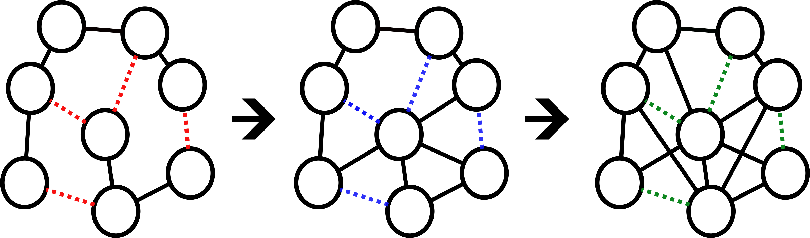
If we consider the graphs in Figure 1 as snapshots pulled from a social network with which a node represents a user and an edge represents a connection between users. Our task is to predict new interactions (the dotted-lines) that will form between existing users. Then, an ideal LP model trained on the first graph would learn a representation that captures the pairwise relations of the connected nodes [11] to make effective predictions. However, this model would likely fail to generalize to the graphs with “blue” and “green” links, since the representations necessary to capture these pairwise relations would require tracking unseen numbers of CNs. To resolve this, our proposed data splitting strategy generates and controls for this scenario in real-world datasets, providing a means from which new models may solve this problem.

Refer to caption — Figure 1: A “realistic” example where sampled edges are represented with dotted lines. The additional edges cause a structural shift where the model learns with more Common Neighbors (CNs). Red = 0 CNs, Blue = 1 CN, Green = 2 CNs.

Furthermore, while numerous methods work to account for distribution shifts within graph machine learning [22], there remains little work doing so for LP. Specifically, we observe that (1) No Benchmark Datasets: Current graph benchmark datasets designed with a quantifiable distribution shift are focused solely on the node and graph tasks [23, 24], with none existing for LP. (2) Absence of Foundational Work: There is no existing work that gives a comprehensive overview of the types of distribution shifts relevant to LP. Current methods are primarily focused on detecting and alleviating anomalies within node- and graph-level tasks [25, 21, 26, 27, 28, 29, 30, 22]. Additionally, few methods exist which are explicitly designed for correcting distribution shift in LP [31, 32, 33, 23]. Also, other LP generalization methods that have been argued to implicitly improve generalization in this shifted scenario remain crucially untested [34, 35].

To tackle these problems, this work proposes the following contributions:

•

Creating Datasets with Meaningful Distribution Shifts. LP requires pairwise structural considerations [1, 36]. Additionally, when considering realistic settings [37] or distribution shift [38], GNN4LP models perform poorly relative to models used in graph [39, 40] and node classification [41, 42]. To better understand distribution shifts, we use key structural LP heuristics to split the links into train/validation/test splits. By using LP heuristics to split the data, we induce shifts in the underlying feature distribution of the links, which are relevant to their existence [36].
•

Benchmarking Current LP Methods. To our surprise, GNN4LP models struggle more than simpler methods when generalizing to data produced by our proposed strategy. Despite the existence of generalization methods that aids link prediction model performance in standard scenarios, there is no means to account for distribution shift and then generalize to our proposed structural distribution shift without re-training the LP model [24, 31, 38]. This reduces the reliability of LP models in-production, since the model will likely to fail to generalize and then require integration into expensive/time-consuming frameworks before re-training on the shifted dataset. This work quantifies the performance of current SOTA LP models and provides analysis for a better foundation to correct this issue. We further quantify the effects of LP generalization methods, finding that they also struggle to generalize to different structural distributions.

The remainder of this paper is structured as follows. In Section 2, we provide background on the heuristics, models, and generalization methods used in LP. In Section 3, we detail how the heuristics relate to our proposed splitting strategy and formally introduce said strategy. Lastly, in Section 4, we benchmark a selection of LP models and generalization methods on our proposed splitting strategy, followed by analysis with the intent of understanding the effects of the new strategy.

2 Related Work

LP Heuristics: Classically, neighborhood heuristics, which measure characteristics between source and target edges, have functioned as the primary means of predicting links. These heuristics show limited effectiveness with a relatively-high variability in results, due to the complicated irregularity within graph datasets, which only grows worse as the dataset grows larger [1]. Regardless of this, state-of-the-art GNN4LP models have integrated these neighborhood heuristics into their architectures to elevate link prediction results [16, 15].

For a given heuristic function, $u$ and $v$ represent the source and target nodes in a potential link $(u,v)$ , $\mathcal{N}(v)$ is the set of all edges connected to the node $v$ , and $f(v_{i,i+1})$ is a function that considers all paths of length $i$ that being at node that starts at $v$ . We consider the following few heuristics:

Common Neighbors [6]: The number of neighbors shared by two nodes $u$ and $v$ ,

\text{CN}(u,v)=|\mathcal{N}(u)\cap\mathcal{N}(v)|.

(1)

Preferential Attachment [1]: The product of the number of neighbors (i.e., the degree) for nodes $u$ and $v$ ,

\text{PA}(u,v)=|\mathcal{N}(u)|\times|\mathcal{N}(v)|.

(2)

Shortest Path Length [1]: The length path between $u$ and $v$ which considers the smallest possible sum $\Sigma$ of length $n-$ nodes,

\text{SP}(u,v)=\operatorname*{arg\,min}_{\Sigma}(\Sigma^{n-1}_{i=1}f(v_{i,i+1})).

(3)

GNNs for Link Prediction (GNN4LP): LP’s current SOTA methods rely on GNNs to constitute a given model’s backbone. The most common choice is the Graph Convolutional Network (GCN) [9], which defines a simplified convolution operator that considers a node’s multi-hop neighborhood. The final score (i.e., probability) of a link existing considers the final representation of both nodes. However, [12] have shown that such methods aren’t suitably expressive for LP, as they ignore vital pairwise information that exists between both nodes. To account for this, SEAL [11] conditions the message passing on both nodes in the target link by applying a node-labelling trick to the enclosed k-hop neighborhood. They demonstrate that this can result in a suitably expressive GNN for LP. NBFNet [43] conditions the message passing on a single node in the target link by parameterizing the generalized Bellman-Ford algorithm. In practice, it’s been shown that conditional message passing is prohibitively expensive to run on many LP datasets [15]. Instead, recent methods pass both the standard GNN representations and an additional pairwise encoding into the scoring function for prediction. For the pairwise encoding, Neo-GNN [44] considers the higher-order overlap between neighborhoods. BUDDY [15] uses the subgraph counts surrounding a target link, which is estimated by using subgraph sketching. Neural Common-Neighbors with Completion (NCNC) [16] encodes the enclosed 1-hop neighborhood of both nodes. Lastly, LPFormer [14] adapts a transformer to learn the pairwise information between two nodes.

Generalization in Link Prediction: Generalization methods for LP rely on a mix of link and node features in order to improve LP model performance. DropEdge [45] randomly removes edges with increasing probability from the training adjacency matrix, allowing for different views of the graph. Edge Proposal Sets (EPS) [34] considers two models – a filter and rank model. The filter model is used to augment the graph with new edges that are likely to be true, while the rank method is used to score the final prediction. [35] defines Topological Concentration (TC), which considers the overlap in subgraph features of a node with each of it’s neighbors. It demonstrates that it correlates well with performance of individual links in LP. To improve the performance of links with a low TC, it considers a re-weighting strategy that places more emphasis on links with a lower TC. Counter-Factual Link Prediction (CFLP) [32] conditions a pre-trained model with edges that contain information counter to the original adjacency matrix. The intent is that the counter-factual links will provide information that is not present in a given dataset.

3 Benchmark Dataset Construction

Algorithm 1 Dataset Splitting Strategy

G=

Initial Graph,

\Psi(.,.)=

Heuristic function

i_{train}

i_{valid}=

Heuristic score thresholds

Train,Valid,Test=\emptyset,\emptyset,\emptyset

6:while edge,

(u,v)

not visited in

G

\Psi(u,v)=h(u,v)

\triangleright

Score edge with neighborhood heuristic

8: if

h(u,v)\leq i_{train}

then

\triangleright

Train Split

Train\leftarrow(u,v)

10: else if

h(u,v)>i_{train}\text{ and }h(u,v)\leq i_{valid}

then

\triangleright

Valid split

11:

Valid\leftarrow(u,v)

12: else

\triangleright

h(u,v)>i_{valid}

, Test Split

13:

Test\leftarrow(u,v)

14: end if

15:end while

16:return

Train,Valid,Test

\triangleright

Return Final Splits

In this section, we attempt to induce a shift in each dataset’s structural features/covariates by proposing a strategy for identifying important structural measures. A structural measure’s importance is determined by how closely-associated it is with how links form within the graph. We further explain how to use these importance measures for generating new splits.

3.1 Types of Distribution Shifts

We consider inducing distribution shifts by splitting the links based on key structural properties which affect link formation and thereby LP. We consider three type of metrics: Local structural information, Global structural information, and Preferential Attachment. Recent work by [46] has shown the importance of local and global structural information for LP. Furthermore, due to the scale-free nature of many real-world graphs and how it relates to link formation [47], we also consider Preferential Attachment. A representative metric is then chosen for each of the three types, shown as follows:

(1) Common Neighbors (CNs): CNs measure local structural information by considering only those nodes connected to the target and source nodes. A real-world case for CNs is whether you share mutual friends with a random person, thus determining if they are your “friend-of-a-friend” [8]. CNs plays a large role in GNN4LP, given that NCNC [16] and EPS [34] integrate CNs into their framework and achieve SOTA performance. Furthermore even on complex real-world datasets, CNs achieves competitive performance against more advanced neural models [17]. To control for the effect of CNs, the relevant splits will consider thresholds which include more CNs.

(2) Shortest Path (SP): SP captures a graph’s global structural information, thanks to the shortest-path between a given target and source node representing the most efficient path for reaching the target [48]. The shift in global structure caused by splitting data with SP can induce a scenario where a model must learn how two dissimilar nodes form a link with one another [49], which is comparable to the real-world scenario where two opponents co-operate with one another [50, 51].

(3) Preferential Attachment (PA): PA captures the scale-free property of larger graphs by multiplying the degrees between two given nodes [47]. When applied to graph generation, PA produces synthetic Barabasi-Albert (BA) graphs which retain the scale-free property to effectively simulate the formation of new links in real-world graphs, such as the World Wide Web [47, 52]. Similar to CNs, the relevant PA splits will consider thresholds that integrate higher PA values.

3.2 Dataset Splitting Strategy

In the last subsection we described the different types of metrics to induce distribution shifts for LP. The metrics cover fundamental structural properties that influence the formation of new links. We now describe how we use these measures to split the dataset into train/validation/test splits to induce such shifts.

In order to build datasets with structural shift, we apply a given neighborhood heuristic to score each link. This score is then compared to a threshold ( $i_{train},i_{valid})$ to categorize a link as a different sample. As denoted in Alg. 1, the heuristic score of the link $(u,v)$ is $h(u,v)$ . The link falls into: training when $h(u,v)<i_{train}$ , validation when $i_{train}\leq h(u,v)<i_{valid}$ , and testing when $h(u,v)>i_{valid}$ . The training graph is constructed from the training edges extracted from the original OGB dataset [17]. Validation and testing samples extracted from this training graph are limited to 100k edges maximum and subsequently removed to prevent test-leakage. The full algorithm is detailed in Algorithm 1 with additional details in Appendix B.

With Figure 2, we provide a small example of how splits are produced by our proposed splitting strategy. Specifically, Figure 2(a) demonstrates the outcome of the CN split labelled “(0,1,2)” where sampled edges pulled from the: black-dotted line = training (no CNs), red-dotted line = validation, (1 CN), and blue-dotted line = testing ( $\geq$ 2 CNs). See Appendix B for information on Figure 2(b) and Figure 2(c).

Finally, to test the effect of different threshold values on performance, we further adjust the $i_{train}$ and $i_{valid}$ thresholds to produce 3 varying splits by CNs and PA and 2 varying splits for the SP thresholds. These variations in splits were chosen based on two conditions. 1) A given sampled edge contains structural information within the user-defined threshold. The core idea is that a training split with a more generous threshold and therefore more structural information will give the model an easier time generalizing to testing samples. 2) The final dataset split contains a sufficient number of samples, so as to provide enough data within each split for a model to generalize to. Given the limited size of the SP split samples and based on condition 2), the SP splits were limited to 2 variants, see Appendix B for more information.

4 Experiments

To bridge the gap for GNN4LP generalizing under distribution shifts, this work addresses the following questions: (RQ1) Can SOTA GNN4LPs generalize under our proposed distribution shifts? (RQ2) Can current LP generalization methods further boost the performance of current methods? and (RQ3) What components of the proposed distribution shift are affecting the LP model’s performance?

4.1 Experimental Setup

Datasets: We consider the ogbl-collab and ogbl-ppa datasets [17] to represent tasks in two different domains, allowing a comprehensive study of the generalization of LP under distribution shift. For both datasets, we create multiple splits corresponding to each structural property detailed in Section 3.2. For the “forward” split, denoted as $(X,Y,Z)$ , an increase in $Y$ and $Z$ indicates more structural information available to the training adjacency matrix. The “inverse” split swaps the training and testing splits from their counterpart in the “forward” split, resulting in the training adjacency matrix losing access to structural information as $X$ and $Y$ increase. See Appendix E for more details.

GNN4LP Methods: We consider multiple SOTA GNN4LP methods including: NCNC [16], BUDDY [15], and LPFormer [14]. We further consider GCN [9] as a simpler GNN baseline. Lastly, we also consider the Resource Allocation (RA) [7] heuristic. Additional models, such as SEAL [12] and Neo-GNN [44] are not considered due to runtime considerations coupled with the relative effectiveness from the variety of currently-selected GNN4LP methods, with differences detailed in Section 2.

Generalization Methods: We also consider enhancing the performance of different LP models with multiple generalization techniques. This includes DropEdge [45], which randomly removes a portion of edges from the training adjacency matrix. Edge Proposal Sets (EPS) [34] utilizes one GNN4LP method to filter edges based on their common neighbors and another method to rank the top-k filtered edges in the training adjacency matrix. Lastly, we consider Topological Concentration (TC) [35], which re-weights the edges within the training adjacency matrix based on the structural information captured by the TC metric. Note: we did not run Counterfactual LP [32] due to experiencing an out-of-memory error on all tested dataset splits.

Evaluation Setting: We consider the standard evaluation procedure in LP, in which every positive validation/test sample is compared against $M$ negative samples. The goal is that the model should output a higher score (i.e., probability) for positive sample than the negatives. To create the negatives, we make use of the HeaRT evaluation setting [37] which generates $M$ negatives samples per positive sample according to a set of common LP heuristics. In our study, we set $M=250$ and use CNs as the heuristic in HeaRT.

Evaluation Metrics: We evaluate all methods using multiple ranking metrics as a standard practice in LP literature [37]. This includes the mean reciprocal rank (MRR) and Hits@20.

Hyperparameters: All methods were tuned on permutations of learning rates in $\{1e^{-2},1e^{-3}\}$ and dropout in $\{0.1,0.3\}$ . Otherwise, we used the recommended hyperparameters for each method according to their official implementations. Each model was trained and tested over five seeds to obtain the mean and standard deviations of their results. Given the significant time complexity of training and testing on the customized ogbl-ppa datasets, NCNC and LPFormer were tuned on a single seed, followed by an evaluation of the tuned model on five separate seeds.

Table 1: ogbl-collab results on the Forward splits. Results reported in MRR with the best bolded and the second best underlined.

Models CN Splits SP Splits PA Splits (0, 1, 2) (0, 2, 4) (0, 3, 5) ( $\infty$ , 6, 4) ( $\infty$ , 4, 3) (0, 50, 100) (0, 100, 200) (0, 150, 250) RA 32.22 29.74 29.86 33.87 33.91 36.87 26.78 24.07 GCN 12.92 ± 0.31 15.20 ± 0.16 17.54 ± 0.19 10.29 ± 0.52 12.94 ± 0.59 20.78 ± 0.25 14.66 ± 0.20 14.03 ± 0.15 BUDDY 17.48 ± 1.19 15.47 ± 0.57 16.60 ± 0.89 16.20 ± 1.40 16.42 ± 2.30 21.27 ± 0.74 14.04 ± 0.76 13.06 ± 0.53 NCNC 9.00 ± 1.02 13.99 ± 1.35 15.04 ± 1.25 14.43 ± 1.36 18.33 ± 1.24 12.76 ± 1.60 6.66 ± 1.24 6.48 ± 1.53 LPFormer 4.27 ± 1.17 13.7 ± 1.48 25.36 ± 2.04 4.6 ± 3.15 15.7 ± 2.87 25.31 ± 5.67 11.98 ± 3.12 12.43 ± 6.62

Table 2: ogbl-ppa results on the Forward splits. Results reported in MRR with the best bolded and the second best underlined.

Models CN Splits SP Splits PA Splits (0, 1, 2) (0, 2, 4) (0, 3, 5) ( $\infty$ , 6, 4) ( $\infty$ , 4, 3) (0, 5k, 10k) (0, 10k, 20k) (0, 15k, 25k) RA 4.71 4.45 4.38 32.57 19.84 3.9 3.14 2.72 GCN 8.13 ± 0.38 7.51 ± 0.32 7.12 ± 1.05 5.40 ± 0.57 5.56 ± 0.21 4.19 ± 0.43 4.98 ± 0.52 5.95 ± 0.28 BUDDY 7.90 ± 0.32 3.83 ± 0.24 3.06 ± 0.06 1.24 ± 0.02 5.87 ± 0.16 3.93 ± 0.98 6.38 ± 3.48 2.48 ± 0.03 NCNC 4.26 ± 0.45 6.87 ± 0.36 6.32 ± 0.57 8.91 ± 7.46 5.55 ± 0.45 8.00 ± 0.60 6.90 ± 1.46 8.00 ± 0.78 LPFormer 3.28 ± 0.63 2.46 ± 0.51 4.84 ± 0.73 9.83 ± 5.92 4.94 ± 0.62 9.27 ± 1.78 9.03 ± 1.6 9.07 ± 2.43

4.2 Results for GNN4LP

In order to provide a unified perspective on how distribution shift affects link prediction models, each GNN4LP method was trained and tested across five seeded runs on versions of ogbl-collab and ogbl-ppa split by Common Neighbors, Shortest-Path, and Preferential-Attachment. Examining the results, we have the two following key observations.

Observation 1: Poor Performance of GNN4LP

As shown in Tables 3, 1, and 2, both RA and GCN consistently out-perform GNN4LP models. In Table 1, RA is overwhelmingly the best-performing, achieving performance more than ten percent higher than the next closest model. However the results for the ogbl-ppa forward split, as shown in Table 2, indicate LPFormer as the best-performing model on the PA split, albeit with a much lower average score than those demonstrated within the ogbl-collab forward split.

Table 3: Mean LP model rank on all splits, determined by Hits@20.

Models	Forward	Inverse
RA	2.06	3.67
GCN	2.75	2.80
BUDDY	3.31	3.33
NCNC	3.44	2.80
LPFormer	3.44	2.40

Given ogbl-ppa’s reduction in performance and the superiority of simpler methods with ogbl-collab, the structural shift induced by our proposed splitting strategy makes it difficult for GNN4LP to generalize. A key consideration for this result is our proposed splitting strategy’s direct effect on graph structure, which implicitly shifts features if structure is correlated to the features, much like how spatio-temporal [33] and size [23] shift affect an input graph.

Table 4: ogbl-collab results on the Inverse splits. Results reported in MRR with the best bolded and the second best underlined.

Models CN Splits SP Splits PA Splits (2, 1, 0) (4, 2, 0) (5, 3, 0) (4, 6, $\infty$ ) (3, 4, $\infty$ ) (100, 50, 0) (200, 100, 0) (250, 150, 0) RA 0.6 4.79 15.9 0.69 0.63 33.09 42.28 44.14 GCN 5.78 ± 0.19 5.91 ± 0.05 7.07 ± 0.11 8.69 ± 0.47 6.47 ± 0.37 21.38 ± 0.27 13.36 ± 0.24 11.95 ± 0.35 BUDDY 3.70 ± 0.13 3.55 ± 0.09 5.40 ± 0.04 6.73 ± 0.32 3.71 ± 0.39 24.95 ± 0.92 15.52 ± 0.73 13.36 ± 0.83 NCNC 1.89 ± 1.27 16.48 ± 1.30 19.69 ± 1.52 1.62 ± 0.72 1.08 ± 0.73 14.86 ± 1.59 18.67 ± 2.75 17.39 ± 2.12 LPFormer 2.01 ± 0.95 3.87 ± 0.74 8.36 ± 0.63 3.16 ± 0.62 1.86 ± 0.48 17.76 ± 2.01 27.56 ± 9.10 24.04 ± 11.35

Table 5: ogbl-ppa results on the Inverse splits. Results reported in MRR with the best bolded and the second best underlined.

Models CN Splits SP Splits PA Splits (2, 1, 0) (4, 2, 0) (5, 3, 0) (4, 6, $\infty$ ) (3, 4, $\infty$ ) (10k, 5k, 0) (20k, 10k, 0) (25k, 15k, 0) RA 0.53 0.92 1.17 0.65 0.54 7.4 5.81 5.08 GCN 3.52 ± 0.09 3.02 ± 0.09 2.94 ± 0.05 10.53 ± 0.48 3.38 ± 0.11 1.55 ± 0.07 1.29 ± 0.02 1.28 ± 0.03 BUDDY 1.60 ± 0.05 2.47 ± 0.07 2.56 ± 0.08 9.91 ± 0.32 3.03 ± 0.06 3.15 ± 0.16 2.55 ± 0.16 2.37 ± 0.02 NCNC 2.37 ± 0.15 8.54 ± 0.74 9.04 ± 0.92 5.56 ± 1.02 1.34 ± 0.56 7.33 ± 0.74 6.02 ± 0.85 5.55 ± 0.77 LPFormer 6.04 ± 0.41 4.23 ± 0.46 3.87 ± 0.1 5.9 ± 1.76 1.38 ± 0.46 14.43 ± 4.45 8.43 ± 3.46 6.27 ± 3.87

Observation 2: Performance Differs By Both Split Type and Thresholds.

As shown in Figure 3, regardless of whether a model is tested on a “Forward” or “Inverse” split; subsequent splits from the same heuristic alter the structural information available across all splits and result in gradual change in the given model’s performance. It is interesting to note that the results for ogbl-ppa and ogbl-collab nearly mirror one another for any given “Forward” split, where an ogbl-ppa split increases the respective ogbl-collab decreases. On the “Inverse” split, a stark increase is seen across most splits, which indicates that increasingly-available structural information in the training adjacency matrix yields improved LP performance [16]. The fact that these results include splits produced by Preferential-Attachment, Global Structural Information, and Local Structural Information further indicates the importance of any structural information when training LP models [46].

4.3 Results for Generalization Methods

In this section, we apply DropEdge [45], EPS [34], and TC [42] on the previously benchmarked GCN [9] and BUDDY [15] to determine the feasibility of LP models’ generalization under our proposed distribution shift.

Table 6: The mean change in performance for all splits for a given generalization methods applied to GCN.

	ogbl-collab			ogbl-ppa
Methods	Forward	Inverse	Overall	Forward	Inverse	Overall
DropEdge	+4%	+2%	+3%	-1%	0%	-0.5%
EPS	-39%	-40%	-40%	-35%	-15%	-25%
TC	-9%	-35%	-22%	0%	0%	0%

Observation 1: LP-Specific Generalization Methods Struggle. As demonstrated in Table 6, the two generalization methods specific to LP: TC [35] and EPS [34] fail to improve the performance of our tested LP models. EPS always results in a decrease of performance from our baseline, indicating a failure to fix the change in performance that our splitting strategy’s structural shift brings. To validate this, we calculate Earth Mover’s Distance (EMD) [53] between the heuristic scores of the training and testing splits. As shown in Figure 4, EPS updates the training adjacency matrix to alter the distance between the sampled distributions; given the results in Table 6, generalizing under our proposed structural shift surpasses the scope of simply updating the training graph’s structure.

TC results in a decrease of performance for ogbl-collab and no change in performance for ogbl-ppa. This is likely due to the thresholds imposed by our strategy which separates splits. There is no distinguishable overlap between sampled distributions: TC can’t re-weight the training adjacency matrix in order to improve LP generalization [35, 54]. This result runs contrary to current work, where re-weighting is effective for handling distribution shifts in other graph tasks [55] and even computer vision [56].

Observation 2: DropEdge Occasionally Works. Additionally, as demonstrated in Table 6, DropEdge [45] is the only generalization method that improves the performance of our tested LP methods on all splits for ogbl-collab, although it has a small detrimental effect on ogbl-ppa. This result is interesting given that DropEdge is not LP-specific and ogbl-collab has an inherent distribution shift involved in predicting unseen author collaborations [17, 33]. However, Figure 4 indicates that DropEdge only has a significant effect on EMD when handling the “Inverse” ogbl-collab CN split, indicating that the performance improvement is due to the change in the adjacency matrix structure, not the change in the distance between sample distributions. Additional EMD results are detailed in the Appendix within Tables 13 and 14.

4.4 Discussion

Does GNN4LP generalize and do LP generalization methods work? As demonstrated by the results of the LP4GNN models and LP generalization methods in Section 4 and relative to their baseline results [17], all tested models fail to generalize and only DropEdge [45] improves LP performance when handling the proposed distribution shift.

How is the proposed distribution shift affecting performance? When considering the EMD calculations for the training and testing samples, it appears that adjustments to the structure of the training adjacency matrix are ineffective for enabling models to generalize under our proposed distribution shift. Regarding the current landscape of LP models and generalization methods, a new framework or architecture, similar to [33], that leverages disentangled learning in regards to structural shift may remedy the problem generated by our proposed dataset splitting strategy.

5 Conclusion

This work proposes a simple dataset splitting strategy for inducing structural shift relevant for link prediction. The effect of this structural shift was then benchmarked on ogbl-collab and ogbl-ppa and shown to pose a unique challenge for current SOTA LP models and generalization methods. Further analysis with EMD calculations demonstrated that generalization under this new structural shift may require techniques which go beyond influencing the structure of the graph data. As such, our proposed dataset splitting strategy provides a new challenge for SOTA LP models and opportunities to expand research for generalizing under structural shifts.

References

[1] David Liben-Nowell and Jon Kleinberg. The link prediction problem for social networks. In Proceedings of the twelfth international conference on Information and knowledge management, pages 556–559, 2003.
[2] Wenqi Fan, Yao Ma, Qing Li, Yuan He, Eric Zhao, Jiliang Tang, and Dawei Yin. Graph neural networks for social recommendation. In The world wide web conference, pages 417–426, 2019.
[3] Yankai Lin, Zhiyuan Liu, Maosong Sun, Yang Liu, and Xuan Zhu. Learning entity and relation embeddings for knowledge graph completion. In Proceedings of the AAAI conference on artificial intelligence, volume 29, 2015.
[4] István A Kovács, Katja Luck, Kerstin Spirohn, Yang Wang, Carl Pollis, Sadie Schlabach, Wenting Bian, Dae-Kyum Kim, Nishka Kishore, Tong Hao, et al. Network-based prediction of protein interactions. Nature communications, 10(1):1240, 2019.
[5] Khushnood Abbas, Alireza Abbasi, Shi Dong, Ling Niu, Laihang Yu, Bolun Chen, Shi-Min Cai, and Qambar Hasan. Application of network link prediction in drug discovery. BMC bioinformatics, 22:1–21, 2021.
[6] Mark EJ Newman. Clustering and preferential attachment in growing networks. Physical review E, 64(2):025102, 2001.
[7] Tao Zhou, Linyuan Lü, and Yi-Cheng Zhang. Predicting missing links via local information. The European Physical Journal B, 71:623–630, 2009.
[8] Lada A Adamic and Eytan Adar. Friends and neighbors on the web. Social networks, 25(3):211–230, 2003.
[9] Thomas N. Kipf and Max Welling. Semi-supervised classification with graph convolutional networks. In International Conference on Learning Representations (ICLR), 2017.
[10] Thomas N Kipf and Max Welling. Variational graph auto-encoders. arXiv preprint arXiv:1611.07308, 2016.
[11] Muhan Zhang and Yixin Chen. Link prediction based on graph neural networks. Advances in neural information processing systems, 31, 2018.
[12] Muhan Zhang, Pan Li, Yinglong Xia, Kai Wang, and Long Jin. Labeling trick: A theory of using graph neural networks for multi-node representation learning. Advances in Neural Information Processing Systems, 34:9061–9073, 2021.
[13] Balasubramaniam Srinivasan and Bruno Ribeiro. On the equivalence between positional node embeddings and structural graph representations. In International Conference on Learning Representations, 2019.
[14] Harry Shomer, Yao Ma, Haitao Mao, Juanhui Li, Bo Wu, and Jiliang Tang. Lpformer: An adaptive graph transformer for link prediction, 2024.
[15] Benjamin Paul Chamberlain, Sergey Shirobokov, Emanuele Rossi, Fabrizio Frasca, Thomas Markovich, Nils Hammerla, Michael M Bronstein, and Max Hansmire. Graph neural networks for link prediction with subgraph sketching. arXiv preprint arXiv:2209.15486, 2022.
[16] Xiyuan Wang, Haotong Yang, and Muhan Zhang. Neural common neighbor with completion for link prediction. In The Twelfth International Conference on Learning Representations, 2023.
[17] Weihua Hu, Matthias Fey, Marinka Zitnik, Yuxiao Dong, Hongyu Ren, Bowen Liu, Michele Catasta, and Jure Leskovec. Open graph benchmark: Datasets for machine learning on graphs. Advances in neural information processing systems, 33:22118–22133, 2020.
[18] Olivia Wiles, Sven Gowal, Florian Stimberg, Sylvestre-Alvise Rebuffi, Ira Ktena, Krishnamurthy Dvijotham, and A. Cemgil. A fine-grained analysis on distribution shift. ArXiv, abs/2110.11328, 2021.
[19] Huaxiu Yao, Caroline Choi, Bochuan Cao, Yoonho Lee, Pang Wei W Koh, and Chelsea Finn. Wild-time: A benchmark of in-the-wild distribution shift over time. In S. Koyejo, S. Mohamed, A. Agarwal, D. Belgrave, K. Cho, and A. Oh, editors, Advances in Neural Information Processing Systems, volume 35, pages 10309–10324. Curran Associates, Inc., 2022.
[20] Huaxiu Yao, Yu Wang, Sai Li, Linjun Zhang, Weixin Liang, James Zou, and Chelsea Finn. Improving out-of-distribution robustness via selective augmentation. In Kamalika Chaudhuri, Stefanie Jegelka, Le Song, Csaba Szepesvari, Gang Niu, and Sivan Sabato, editors, Proceedings of the 39th International Conference on Machine Learning, volume 162 of Proceedings of Machine Learning Research, pages 25407–25437. PMLR, 17–23 Jul 2022.
[21] Beatrice Bevilacqua, Yangze Zhou, and Bruno Ribeiro. Size-invariant graph representations for graph classification extrapolations. In International Conference on Machine Learning, pages 837–851. PMLR, 2021.
[22] Haoyang Li, Xin Wang, Ziwei Zhang, and Wenwu Zhu. Out-of-distribution generalization on graphs: A survey. arXiv preprint arXiv:2202.07987, 2022.
[23] Yangze Zhou, Gitta Kutyniok, and Bruno Ribeiro. Ood link prediction generalization capabilities of message-passing gnns in larger test graphs. Advances in Neural Information Processing Systems, 35:20257–20272, 2022.
[24] Mucong Ding, Kezhi Kong, Jiuhai Chen, John Kirchenbauer, Micah Goldblum, David Wipf, Furong Huang, and Tom Goldstein. A closer look at distribution shifts and out-of-distribution generalization on graphs. In NeurIPS 2021 Workshop on Distribution Shifts: Connecting Methods and Applications, 2021.
[25] Wei Jin, Tong Zhao, Jiayuan Ding, Yozen Liu, Jiliang Tang, and Neil Shah. Empowering graph representation learning with test-time graph transformation. arXiv preprint arXiv:2210.03561, 2022.
[26] Yuan Gao, Xiang Wang, Xiangnan He, Zhenguang Liu, Huamin Feng, and Yongdong Zhang. Alleviating structural distribution shift in graph anomaly detection. In Proceedings of the Sixteenth ACM International Conference on Web Search and Data Mining, pages 357–365, 2023.
[27] Qitian Wu, Fan Nie, Chenxiao Yang, Tianyi Bao, and Junchi Yan. Graph out-of-distribution generalization via causal intervention. In Proceedings of the ACM on Web Conference 2024, pages 850–860, 2024.
[28] Yuxin Guo, Cheng Yang, Yuluo Chen, Jixi Liu, Chuan Shi, and Junping Du. A data-centric framework to endow graph neural networks with out-of-distribution detection ability. In Proceedings of the 29th ACM SIGKDD Conference on Knowledge Discovery and Data Mining, pages 638–648, 2023.
[29] Qitian Wu, Yiting Chen, Chenxiao Yang, and Junchi Yan. Energy-based out-of-distribution detection for graph neural networks. arXiv preprint arXiv:2302.02914, 2023.
[30] Yongduo Sui, Qitian Wu, Jiancan Wu, Qing Cui, Longfei Li, Jun Zhou, Xiang Wang, and Xiangnan He. Unleashing the power of graph data augmentation on covariate distribution shift. Advances in Neural Information Processing Systems, 36, 2024.
[31] Kaiwen Dong, Yijun Tian, Zhichun Guo, Yang Yang, and Nitesh Chawla. Fakeedge: Alleviate dataset shift in link prediction. In Learning on Graphs Conference, pages 56–1. PMLR, 2022.
[32] Tong Zhao, Gang Liu, Daheng Wang, Wenhao Yu, and Meng Jiang. Learning from counterfactual links for link prediction. In International Conference on Machine Learning, pages 26911–26926. PMLR, 2022.
[33] Zeyang Zhang, Xin Wang, Ziwei Zhang, Haoyang Li, Zhou Qin, and Wenwu Zhu. Dynamic graph neural networks under spatio-temporal distribution shift. Advances in neural information processing systems, 35:6074–6089, 2022.
[34] Abhay Singh, Qian Huang, Sijia Linda Huang, Omkar Bhalerao, Horace He, Ser-Nam Lim, and Austin R Benson. Edge proposal sets for link prediction. arXiv preprint arXiv:2106.15810, 2021.
[35] Yu Wang, Tong Zhao, Yuying Zhao, Yunchao Liu, Xueqi Cheng, Neil Shah, and Tyler Derr. A topological perspective on demystifying gnn-based link prediction performance. arXiv preprint arXiv:2310.04612, 2023.
[36] Haitao Mao, Zhikai Chen, Wei Jin, Haoyu Han, Yao Ma, Tong Zhao, Neil Shah, and Jiliang Tang. Demystifying structural disparity in graph neural networks: Can one size fit all? Advances in Neural Information Processing Systems, 36, 2024.
[37] Juanhui Li, Harry Shomer, Haitao Mao, Shenglai Zeng, Yao Ma, Neil Shah, Jiliang Tang, and Dawei Yin. Evaluating graph neural networks for link prediction: Current pitfalls and new benchmarking. Advances in Neural Information Processing Systems, 36, 2024.
[38] Jing Zhu, Yuhang Zhou, Vassilis N Ioannidis, Shengyi Qian, Wei Ai, Xiang Song, and Danai Koutra. Pitfalls in link prediction with graph neural networks: Understanding the impact of target-link inclusion & better practices. In Proceedings of the 17th ACM International Conference on Web Search and Data Mining, pages 994–1002, 2024.
[39] Lanning Wei, Huan Zhao, Quanming Yao, and Zhiqiang He. Pooling architecture search for graph classification. In Proceedings of the 30th ACM International Conference on Information and Knowledge Management, CIKM ’21. ACM, October 2021.
[40] Zhuoning Yuan, Yan Yan, Milan Sonka, and Tianbao Yang. Large-scale robust deep auc maximization: A new surrogate loss and empirical studies on medical image classification, 2021.
[41] Zhihao Shi, Jie Wang, Fanghua Lu, Hanzhu Chen, Defu Lian, Zheng Wang, Jieping Ye, and Feng Wu. Label deconvolution for node representation learning on large-scale attributed graphs against learning bias. arXiv preprint arXiv:2309.14907, 2023.
[42] Jianan Zhao, Meng Qu, Chaozhuo Li, Hao Yan, Qian Liu, Rui Li, Xing Xie, and Jian Tang. Learning on large-scale text-attributed graphs via variational inference, 2023.
[43] Zhaocheng Zhu, Zuobai Zhang, Louis-Pascal Xhonneux, and Jian Tang. Neural bellman-ford networks: A general graph neural network framework for link prediction. Advances in Neural Information Processing Systems, 34:29476–29490, 2021.
[44] Seongjun Yun, Seoyoon Kim, Junhyun Lee, Jaewoo Kang, and Hyunwoo J Kim. Neo-gnns: Neighborhood overlap-aware graph neural networks for link prediction. Advances in Neural Information Processing Systems, 34:13683–13694, 2021.
[45] Yu Rong, Wenbing Huang, Tingyang Xu, and Junzhou Huang. Dropedge: Towards deep graph convolutional networks on node classification. In International Conference on Learning Representations, 2020.
[46] Haitao Mao, Juanhui Li, Harry Shomer, Bingheng Li, Wenqi Fan, Yao Ma, Tong Zhao, Neil Shah, and Jiliang Tang. Revisiting link prediction: A data perspective. arXiv preprint arXiv:2310.00793, 2023.
[47] Albert-László Barabási and Réka Albert. Emergence of scaling in random networks. Science, 286(5439):509–512, 1999.
[48] Stuart Russell and Peter Norvig. Artificial Intelligence: A Modern Approach. Prentice Hall Press, USA, 3rd edition, 2009.
[49] Anna Evtushenko and Jon Kleinberg. The paradox of second-order homophily in networks. Scientific Reports, 11(1):13360, 2021.
[50] Thomas C Schelling. Micromotives and macrobehavior ww norton & company. New York, NY, 1978.
[51] Mark Granovetter. Threshold models of collective behavior. American journal of sociology, 83(6):1420–1443, 1978.
[52] Réka Albert and Albert-László Barabási. Statistical mechanics of complex networks. Reviews of Modern Physics, 74(1):47–97, January 2002.
[53] Y. Rubner, C. Tomasi, and L.J. Guibas. A metric for distributions with applications to image databases. In Sixth International Conference on Computer Vision (IEEE Cat. No.98CH36271), pages 59–66, 1998.
[54] Haoyang Li, Xin Wang, Ziwei Zhang, and Wenwu Zhu. Ood-gnn: Out-of-distribution generalized graph neural network. IEEE Transactions on Knowledge and Data Engineering, 2022.
[55] Xiao Zhou, Yong Lin, Renjie Pi, Weizhong Zhang, Renzhe Xu, Peng Cui, and Tong Zhang. Model agnostic sample reweighting for out-of-distribution learning. In International Conference on Machine Learning, pages 27203–27221. PMLR, 2022.
[56] Tongtong Fang, Nan Lu, Gang Niu, and Masashi Sugiyama. Rethinking importance weighting for deep learning under distribution shift. Advances in neural information processing systems, 33:11996–12007, 2020.

Checklist

1.
For all authors…
1. (a)
  
  Do the main claims made in the abstract and introduction accurately reflect the paper’s contributions and scope? [Yes]
2. (b)
  
  Did you describe the limitations of your work? [Yes] See Appendix G.
3. (c)
  
  Did you discuss any potential negative societal impacts of your work? [Yes] See Appendix H.
4. (d)
  
  Have you read the ethics review guidelines and ensured that your paper conforms to them? [Yes]
2.
If you are including theoretical results…
1. (a)
  
  Did you state the full set of assumptions of all theoretical results? [N/A]
2. (b)
  
  Did you include complete proofs of all theoretical results? [N/A]
3.
If you ran experiments (e.g. for benchmarks)…
1. (a)
  
  Did you include the code, data, and instructions needed to reproduce the main experimental results (either in the supplemental material or as a URL)? [Yes] See https://github.com/revolins/LPStructGen.
2. (b)
  
  Did you specify all the training details (e.g., data splits, hyperparameters, how they were chosen)? [Yes] See Section 4.1 and Appendix E.
3. (c)
  
  Did you report error bars (e.g., with respect to the random seed after running experiments multiple times)? [Yes]
4. (d)
  
  Did you include the total amount of compute and the type of resources used (e.g., type of GPUs, internal cluster, or cloud provider)? [Yes] See, Appendix E.
4.
If you are using existing assets (e.g., code, data, models) or curating/releasing new assets…
1. (a)
  
  If your work uses existing assets, did you cite the creators? [Yes]
2. (b)
  
  Did you mention the license of the assets? [Yes] See Appendix F.
3. (c)
  
  Did you include any new assets either in the supplemental material or as a URL? [Yes] See https://github.com/revolins/LPStructGen.
4. (d)
  
  Did you discuss whether and how consent was obtained from people whose data you’re using/curating? [Yes] See Appendix F.
5. (e)
  
  Did you discuss whether the data you are using/curating contains personally identifiable information or offensive content? [N/A]
5.
If you used crowdsourcing or conducted research with human subjects…
1. (a)
  
  Did you include the full text of instructions given to participants and screenshots, if applicable? [N/A]
2. (b)
  
  Did you describe any potential participant risks, with links to Institutional Review Board (IRB) approvals, if applicable? [N/A]
3. (c)
  
  Did you include the estimated hourly wage paid to participants and the total amount spent on participant compensation? [N/A]

Appendix A Heuristic Choice

Resource Allocation and Adamic-Adar Index were not considered for splitting strategies given that they build upon the original Common Neighbor formulation. We acknowledge this may lead to interesting analysis on how higher-order heuristics could influence distribution shifts, however it is redundant given our intentions to induce distinct structural scenarios to the test LP models using just link prediction heuristics for splitting strategies.

Appendix B Splitting Strategy – Additional Algorithmic Details

This section provides additional details about the way data was formatted before being used as input for Algorithm 1 of our proposed splitting strategy and the intuition behind how Preferential-Attachment and Shortest-Path work within the splitting strategy. The details on the algorithm includes:

•

Validation and Testing Edges are limited to 100k edges total.
•

PPA Training Edges are limited to 3 million edges total.
•

Negative Testing and Validation edges are produced via HeaRT [37].
•

Validation and testing edges that are duplicated with training edges are removed from the edge index.
•

In order to provide overlap within a given dataset, validation and testing edges that do not connect to training nodes are removed from the edge index.
•

After sampling the necessary training edges, the adjacency matrix is extracted from the edge index, converted to an undirected graph and has any edge weights standardized to 1.

Common Neighbors, Preferential-Attachment and Shortest-Path, as shown in Figure 2(a), 2(b), and 2(c) respectively, are interchangeable within the dataset splitting strategy. Details about how Common Neighbors functions within the strategy are included in Section 3.2. Figure 2(b) and Figure 2(c) serve as toy examples and do not correspond directly to any dataset splits tested within our study. However, the examples illustrated within Figure 2(b) and Figure 2(c) do correspond to how their given heuristic functions within our splitting strategy.

For Figure 2(b) or Preferential-Attachment, it determines the degrees between a given source and target node and then multiples the two to produce the score, based on that score, the sample is then sorted into a new dataset split.

For Figure 2(c) or Shortest-Path, the heuristic determines the score by determining the minimum number of nodes necessary to reach the target node from the source node. If there is a link between the two nodes, we remove the link and then re-add to the adjacency matrix after the score calculation. The final Shortest-Path score applies the calculated shortest-path length, $SP(u,v)$ as the denominator in a ratio of $\frac{1}{SP(u,v)}$ , which is then used to sort the sample into it’s respective dataset split.

Appendix C Size of Dataset Samples

In this section we detail the number of training, validation, and test edges for all of the newly created splits detailed in Section 3. There are in Tables 7 and 8 for ogbl-collab and ogbl-ppa, respectively.

Table 7: Number of samples in the ogbl-collab dataset for the forward and backward heuristic splits, separated into columns allocated for training, validation, and testing splits.

Heuristic	Split	Train	Valid	Test
CN	(0, 1, 2)	57638	6920	4326
	(0, 2, 4)	237928	20045	14143
	(0, 3, 5)	493790	31676	21555
	(2, 1, 0)	1697336	23669	9048
	(4, 2, 0)	1193456	24097	11551
	(5, 3, 0)	985820	25261	11760
SP	( $\infty$ , 6, 4)	46880	1026	2759
	( $\infty$ , 4, 3)	52872	1238	3457
	(4, 6, $\infty$ )	1882392	5222	2626
	(3, 4, $\infty$ )	1877626	4384	7828
PA	(0, 50, 100)	210465	46626	9492
	(0, 100, 200)	329383	62868	25527
	(0, 150, 250)	409729	75980	39429
	(100, 50, 0)	1882392	5222	2626
	(200, 100, 0)	1877626	4384	7828
	(250, 150, 0)	457372	65323	30999

Table 8: Number of samples in the ogbl-ppa dataset for the forward and backward heuristic splits, separated into columns allocated for training, validation, and testing splits

Heuristic	Split	Train	Valid	Test
CN	(0, 1, 2)	2325936	87880	67176
	(0, 2, 4)	3000000	95679	83198
	(0, 3, 5)	3000000	98081	88778
	(2, 1, 0)	3000000	96765	92798
	(4, 2, 0)	3000000	93210	85448
	(5, 3, 0)	3000000	92403	81887
SP	( $\infty$ , 6, 4)	17464	149	20
	( $\infty$ , 4, 3)	134728	4196	1180
	(4, 6, $\infty$ )	3000000	90511	458
	(3, 4, $\infty$ )	3000000	97121	74068
PA	(0, 5k, 10k)	95671	95671	45251
	(0, 10k, 20k)	98562	98562	63178
	(0, 15k, 25k)	99352	99352	72382
	(10k, 5k, 0)	3000000	90623	44593
	(20k, 10k, 0)	3000000	89671	34321
	(25k, 15k, 0)	3000000	91995	35088

Appendix D Dataset Results

In this section, we include all of the results for each experiment conducted on the generalization methods and EMD calculations. Results from Tables 9, 10, 11, and 12 were used for the calculations demonstrated in Figure 6. Figure 4 was constructed from results within Table 13.

Table 9: ogbl-collab results on the forward and inverse splits when using DropEdge and TC.

		DropEdge		TC
Heuristic	Split	GCN	BUDDY	GCN	BUDDY
CN	(0, 1, 2)	13.92 ± 0.78	15.54 ± 0.98	12.26± 0.28	11.27 ± 2.03
	(0, 2, 4)	15.85 ± 0.25	16.16 ± 0.17	12.62± 0.57	12.39 ± 1.43
	(0, 3, 5)	17.75 ± 0.11	16.34 ± 0.17	13.3± 0.47	14.99 ± 1.69
	(2, 1, 0)	5.96 ± 0.17	2.61 ± 0.09	4.95 ±0.16	5.28 ± 0.05
	(4, 2, 0)	6.14 ± 0.065	2.88 ± 0.11	5.37 ±0.13	5.23 ± 0.05
	(5, 3, 0)	7.20 ± 0.15	4.99 ± 0.08	6.04± 0.07	6.03 ± 0.10
SP	( $\infty$ , 6, 4)	11.94 ± 0.46	12.31 ± 0.51	11.42 ±0.43	7.25 ± 0.81
	( $\infty$ , 4, 3)	13.87 ± 0.43	17.11 ± 1.02	12.88± 0.43	9.33 ± 1.66
	(4, 6, $\infty$ )	9.18 ± 0.52	5.34 ± 0.43	9.09± 4.74	6.88 ± 0.30
	(3, 4, $\infty$ )	6.71 ± 0.13	2.93 ± 0.18	3.57± 2.30	6.24 ± 0.13
PA	(0, 50, 100)	20.76 ± 0.19	21.35 ± 0.36	17.55±0.57	18.82 ± 1.35
	(0, 100, 200)	14.57 ± 0.20	13.84 ± 0.64	13.22±1.1	12.13±1.04
	(0, 150, 250)	13.78 ± 0.28	12.85 ± 0.78	13.03±0.24	10.63±0.55
	(100, 50, 0)	21.34 ± 0.65	26.09 ± 0.62	6.4 ± 0.2	15.84 ± 1.13
	(200, 100, 0)	12.89 ± 0.59	15.68 ± 0.85	4.3 ± 0.14	9.15 ± 0.39
	(250, 150, 0)	11.68 ± 0.37	13.13 ± 0.94	4.4 ± 0.16	6.7 ± 0.2

Table 10: ogbl-ppa results on the forward and inverse splits when using DropEdge and TC.

		DropEdge		TC
Heuristic	Split	GCN	BUDDY	GCN	BUDDY
CN	(0, 1, 2)	8.20 ± 0.34	7.83 ± 0.27	OOM	5.27 ± 0.34
	(0, 2, 4)	7.39 ± 0.33	3.83 ± 0.25	OOM	2.91 ± 0.06
	(0, 3, 5)	6.04 ± 0.32	3.06 ± 0.06	OOM	2.67 ± 0.13
	(2, 1, 0)	3.50 ± 0.16	1.61 ± 0.04	OOM	3.44 ± 0.08
	(4, 2, 0)	3.01 ± 0.07	2.47 ± 0.07	OOM	3.45 ± 0.1
	(5, 3, 0)	2.97 ± 0.06	2.56 ± 0.08	OOM	3.55 ± 0.13
SP	( $\infty$ , 6, 4)	6.17 ± 0.76	3.86 ± 0.39	OOM	4.0 ± 0.29
	( $\infty$ , 4, 3)	5.55 ± 0.22	5.87 ± 0.16	OOM	4.82 ± 0.39
	(4, 6, $\infty$ )	3.44 ± 0.17	3.86 ± 0.39	OOM	13.2 ± 0.45
	(3, 4, $\infty$ )	15.69 ± 0.54	5.87 ± 0.16	OOM	2.89 ± 0.09
PA	(0, 50, 100)	4.19 ± 0.43	3.93 ± 0.98	OOM	3.62 ± 0.21
	(0, 10k, 20k)	4.98 ± 0.52	6.38 ± 3.48	OOM	3.13 ± 0.12
	(0, 15k, 25k)	5.95 ± 0.28	2.49 ± 0.01	OOM	3.33 ± 1.38
	(10k, 5k, 0)	1.51 ± 0.02	3.13 ± 0.1	OOM	1.78 ± 0.16
	(20k, 10k, 0)	1.25 ± 0.07	2.56 ± 0.19	OOM	1.5 ± 0.0008
	(25k, 15k, 0)	1.28 ± 0.03	2.40 ± 0.03	OOM	1.53 ± 0.04

Table 11: ogbl-collab results on the forward and inverse splits when using EPS for each given Filter + Rank model configuration.

Heuristic	Split	GCN + BUDDY	BUDDY + GCN	RA + GCN	RA + BUDDY
CN	(0, 1, 2)	8.50 ± 1.10	5.81 ± 0.11	7.42 ± 0.12	3.94 ± 0.51
	(0, 2, 4)	12.85 ± 0.83	5.31 ± 0.22	7.07 ± 0.16	6.61 ± 0.30
	(0, 3, 5)	15.35 ± 0.96	5.88 ± 0.16	7.52 ± 0.13	7.16 ± 0.09
	(2, 1, 0)	5.46 ± 0.11	4.90 ± 0.08	5.24 ± 0.14	4.32 ± 0.19
	(4, 2, 0)	5.36 ± 0.12	4.62 ± 0.16	5.27 ± 0.09	4.45 ± 0.12
	(5, 3, 0)	5.96 ± 0.06	5.17 ± 0.09	5.15 ± 0.26	4.93 ± 0.11
SP	( $\infty$ , 6, 4)	7.38 ± 0.82	7.10 ± 0.43	7.38 ± 0.42	3.84 ± 0.59
	( $\infty$ , 4, 3)	9.60 ± 0.39	6.24 ± 0.52	7.07 ± 0.46	7.63 ± 0.25
	(4, 6, $\infty$ )	6.86 ± 1.13	6.51 ± 0.24	6.11 ± 0.48	6.86 ± 1.13
	(3, 4, $\infty$ )	6.47 ± 0.24	4.86 ± 0.38	5.23 ± 0.23	6.47 ± 0.24
PA	(0, 50, 100)	15.92 ± 1.01	13.84 ± 0.14	13.23 ± 0.21	15.92 ± 1.01
	(0, 100, 200)	9.47 ± 0.31	10.85 ± 0.11	10.71 ± 0.10	9.47 ± 0.31
	(0, 150, 250)	9.60 ± 0.41	10.33 ± 0.15	9.96 ± 0.06	9.60 ± 0.41
	(100, 50, 0)	14.34 ± 1.05	5.23 ± 0.28	5.07 ± 0.21	14.34 ± 1.05
	(200, 100, 0)	8.35 ± 0.34	3.06 ± 0.08	2.93 ± 0.06	8.35 ± 0.34
	(250, 150, 0)	5.50 ± 0.33	3.14 ± 0.14	2.79 ± 0.07	5.50 ± 0.33

Table 12: ogbl-ppa results on the forward and inverse splits when using EPS for each given Filter + Rank model configuration.

Heuristic	Split	GCN + BUDDY	BUDDY + GCN	RA + GCN	RA + BUDDY
CN	(0, 1, 2)	4.48 ± 0.33	OOM	3.53 ± 0.03	4.04 ± 0.26
	(0, 2, 4)	3.79 ± 0.28	OOM	3.35 ± 0.03	3.42 ± 0.20
	(0, 3, 5)	3.16 ± 0.10	OOM	3.22 ± 0.04	2.95 ± 0.13
	(2, 1, 0)	3.19 ± 0.08	OOM	2.79 ± 0.11	2.58 ± 0.09
	(4, 2, 0)	3.25 ± 0.09	OOM	2.64 ± 0.02	3.04 ± 0.05
	(5, 3, 0)	3.36 ± 0.13	OOM	2.55 ± 0.09	3.10 ± 0.15
SP	( $\infty$ , 6, 4)	4.00 ± 0.20	OOM	2.09 ± 0.17	3.89 ± 0.23
	( $\infty$ , 4, 3)	5.53 ± 0.92	OOM	5.18 ± 0.51	5.53 ± 0.94
	(4, 6, $\infty$ )	14.41 ± 0.67	OOM	6.46 ± 0.84	13.63 ± 0.97
	(3, 4, $\infty$ )	2.93 ± 0.15	OOM	2.48 ± 0.06	2.51 ± 0.14
PA	(0, 50, 100)	3.66 ± 0.38	OOM	4.34 ± 0.06	3.66 ± 0.38
	(0, 100, 200)	3.19 ± 0.22	OOM	4.23 ± 0.03	3.19 ± 0.22
	(0, 150, 250)	2.88 ± 0.06	OOM	3.78 ± 0.07	2.88 ± 0.06
	(100, 50, 0)	2.05 ± 0.05	OOM	1.43 ± 0.05	2.05 ± 0.04
	(200, 100, 0)	1.67 ± 0.03	OOM	1.26 ± 0.02	1.65 ± 0.05
	(250, 150, 0)	1.66 ± 0.02	OOM	1.30 ± 0.02	1.64 ± 0.03

Table 13: EMD calculations for ogbl-collab on the forward and inverse splits. Scores with a distance multiple-times different than the baseline are in bold

Heuristic	Split	Baseline	DropEdge	EPS - GCN	EPS - BUDDY
CN	(0, 1, 2)	1.31	1.31	6.62	3.6
	(0, 2, 4)	1.6	1.6	4.91	2.52
	(0, 3, 5)	1.45	1.65	3.82	2.22
	(2, 1, 0)	1.87	1.15	1.71	2.91
	(4, 2, 0)	2.26	1.49	1.29	2.99
	(5, 3, 0)	2.28	1.52	0.314	2.14
SP	( $\infty$ , 6, 4)	5.93	5.94	0.012	0.012
	( $\infty$ , 4, 3)	5.35	5.38	0.002	0.003
	(4, 6, $\infty$ )	3.6	3.53	1.22	1.22
	(3, 4, $\infty$ )	1.85	1.78	3.17	3.23
PA	(0, 50, 100)	1.87	1.89	2.94	3.42
	(0, 100, 200)	2.29	2.32	3.59	2.72
	(0, 150, 250)	2.34	2.36	3.73	3.08
	(100, 50, 0)	4.29	4.3	3.31	2.48
	(200, 100, 0)	3.79	3.82	2.84	0.78
	(250, 150, 0)	3.48	3.5	2.7	2.48

Table 14: EMD calculations for ogbl-ppa on the forward and inverse splits.

Heuristic	Split	Baseline	DropEdge	EPS
CN	(0, 1, 2)	2.82	2.82	>24hrs
	(0, 2, 4)	3.13	3.13	>24hrs
	(0, 3, 5)	3.05	3.19	>24hrs
	(2, 1, 0)	3.1	2.36	>24hrs
	(4, 2, 0)	3.3	2.55	>24hrs
	(5, 3, 0)	3.19	2.44	>24hrs
SP	( $\infty$ , 6, 4)	5.81	5.84	>24hrs
	( $\infty$ , 4, 3)	1.36	1.4	>24hrs
	(4, 6, $\infty$ )	2.14	2.14	>24hrs
	(3, 4, $\infty$ )	0.72	0.72	>24hrs
PA	(0, 5k, 10k)	2.55	2.55	>24hrs
	(0, 10k, 20k)	2.76	2.76	>24hrs
	(0, 15k, 25k)	2.78	2.78	>24hrs
	(10k, 5k, 0)	2.96	2.96	>24hrs
	(20k, 10k, 0)	2.68	2.68	>24hrs
	(25k, 15k, 0)	2.48	2.48	>24hrs

Appendix E Additional Training Details

This section provides relevant details about training and reproducing results not mentioned in Section 4.1:

•

NCNC for all datasets and splits, besides the ogbl-ppa PA splits, considers the ’NCNC2’ variant of NCNC with an added depth argument of 2 [16]. For the ogbl-ppa PA splits, we apply a depth argument of just 1 in order to ensure that a single seeded run does not exceed 24 hour runtime.
•

All experiments were conducted with a single A6000 48GB GPU and 1TB of available system RAM.
•

Please consult the project README for building the project, loading data, and re-creating results.

Appendix F Dataset Licenses

The dataset splitting strategy proposed in this paper is built using Pytorch Geometric (PyG). As such, this project’s software and the PyG datasets are freely-available under the MIT license.

Appendix G Limitations

The proposed dataset splitting strategy is restricted to inducing distribution shifts solely with neighborhood heuristics. So, it does not consider other types of distribution shifts that are possible within the link prediction task (i.e. spatio-temporal [33] or size [23] shift). Additionally, since the neighborhood heuristics compute discrete scores produced from an input graph’s structural information and effectively training GNN4LP models requires no leakage with validation/testing, it may be difficult to determine the correct thresholds to extract a meaningful number of samples. For Common Neighbors and Preferential-Attachment, this is especially relevant with smaller training graphs, given that larger and/or denser graphs have inherently more edges. Therefore, larger and denser graphs have inherently more possible Common Neighbors and Preferential-Attachment scores. For Shortest-Path, splitting can be exceptionally difficult for denser graphs, as demonstrated with the tiny split sizes for ogbl-ppa in Table 8.

Appendix H Impact Statement

Our proposed dataset splitting strategy mimics the formatting of PyTorch Geometric datasets. This means that our strategy is simple to implement, enabling future work involved with understanding this type of structural shift for link prediction and promoting beginner-friendly practices for artificial intelligence research. Additionally, since the structural shift we propose in this article affects real-life systems, which integrate link prediction models, this research can provide a foundation for the improvement of relevant technologies; which holds positive ramifications for society and future research. No apparent risk is related to the contribution of this work.

Appendix I Exclusion of non-LP Generalization Methods

Given that this study is focused on elevating the current understanding for how link prediction models handle the generalized-case of structural shift, our focus was on two objectives: 1) producing and then benchmarking meaningful dataset splits relevant to structural shift in LP, 2) improving understanding on whether generalization methods specifically designed for LP aid GNN4LP on datasets shifted by our proposed splitting strategy. Given the lack of testing for LP-specific generalization methods under any form of distribution shift, our focus on 2) is especially pertinent in order to improve understanding on how LP-specific generalization methods aid performance under distribution shift. We refer readers to [33] for more information on how non-specific generalization methods aid performance for link prediction models under spatio-temporal shift.