Unconventional Quantum Electrodynamics with Hofstadter-Ladder Waveguide
Abstract
We propose a novel quantum electrodynamics (QED) platform where quantum emitters interact with a Hofstadter-ladder waveguide. We demonstrate several intriguing phenomena stemming from the nontrivial dispersion relation and vacuum mode properties led by the effective spin-orbit coupling. First, by assuming emitter’s frequency to be resonant with the lower band, we find that the spontaneous emission is chiral with most photonic field decaying unidirectionally. Both numerical and analytical results indicate that the Hofstadter-ladder waveguide can be engineered as a well-performed chiral quantum bus. Second, the dynamics of emitters of giant atom form is explored by considering their frequencies below the lower band. Due to quantum interference, we find that both the emitter-waveguide interaction and the amplitudes of bound states are periodically modulated by giant emitter’s size. The periodical length depends on the positions of energy minima points induced by the spin-orbit coupling. Last, we consider the interaction between two giant emitters mediated by bound states, and find that their dipole-dipole interaction vanishes (is enhanced) when maximum destructive (constructive) interference happens.
I introduction
The interactions between quantum emitters and the unavoidable baths with large degrees of freedom are the central topic of quantum optics Cohen-Tannoudji et al. (1998); Clerk et al. (2010). For example, in the present of a vacuum bath, the emitter will spontaneously decay to its ground state as well as its frequency being renormalized due to Lamb shifts Lamb and Retherford (1947); Scully and Zubairy (1997). By shaping the size of the environment or narrowing its spectrum bandwidth, many intriguing phenomena, such as isotropic propagation of photons and non-Markovian evolution arise John and Quang (1994); Lambropoulos et al. (2000); Giraldi and Petruccione (2011); Lodahl et al. (2015); Stewart et al. (2020); Ferreira et al. (2021). As discussed in Refs. Petersen et al. (2014); Bliokh and Nori (2015); Bliokh et al. (2015); Lodahl et al. (2017); Lang et al. (2022), chiral emission can be observed via the subwavelength confinement in nanophotonic systems, which opens the possibilities to realize cascaded quantum networks. Moreover, when considering an emitter coupling to the bandgaps of a bath John and Wang (1990); Goban et al. (2014); González-Tudela et al. (2015); Douglas et al. (2016); Liu and Houck (2017); Chang et al. (2018); Wang et al. (2021a), photonic bound states (in the form of an evanescent field) emerge Douglas et al. (2015). In this scenario, between atoms there are long-range dipole-dipole interactions by exchanging the virtual photons in the waveguide Shahmoon and Kurizki (2013); Ying et al. (2019).
In recent years, exploring quantum electrodynamics (QED) with emitters coupling to structured lattice environments, has attracted a lot of interests Ramos et al. (2016); Calajo et al. (2016); González-Tudela and Cirac (2018); González-Tudela et al. (2019); Leonforte et al. (2021). Those artificial lattice reservoirs are widely studied in condensed matter physics, and usually have unconventional spectra, or topological properties with nontrivial vacuum modes. In Refs. González-Tudela and Cirac (2017, 2017), by considering emitters interacting with a 2D tight-binding lattice environment, the authors showed that both superradiance and subradiance of collective atoms emerge in the nonperturbative regime. The unusual chiral bound states and directional dipole-dipole interaction were also demonstrated in a topological waveguide QED system Bello et al. (2019); Kim et al. (2021). In Refs. Roccati et al. (2022); Gong et al. (2022), the authors discussed how to realize bound states and dipole-dipole interactions in non-Hermitian photonic lattices. All these studies indicate those structured lattice reservoirs with reduced dimensionality are versatile toolboxes for exploring novel quantum optical phenomena, as well as the potential applications in quantum information processing.
In artificial baths with the spin-orbit coupling, the motion and spin freedoms of a particle are linked, and many anomalous phenomena such as spin-Hall effect and topological insulators can be observed Zhang (2000); Murakami et al. (2003); Sinova et al. (2004); Wunderlich et al. (2005); Kane and Mele (2005); Galitski and Spielman (2013); Zhou et al. (2013); Wu et al. (2016); Kartashov et al. (2017); Livi et al. (2016); Liu et al. (2011). Since neither the spin nor the momentum is the well-defined quantum number to describe the dispersion relation, the spin-orbit coupling will produce nontrivial energy bands and photonic modes Sala et al. (2015); Salerno et al. (2017). The quantum optics with emitters interacting with baths of the spin-orbit coupling, is rarely studied. It is a simple but interesting toy model in condensed matter physics (see Fig. 1) Creutz (2001); Narozhny et al. (2005); Jaefari and Fradkin (2012); Atala et al. (2014); Tai et al. (2017); Yuan et al. (2019); Guan et al. (2020). As discussed in Ref. Hügel and Paredes (2014), the ladder contains two legs which play the roles of two freedoms in an effective spin. In the present of synthetic gauge fields, the effective spin will be locked to momentum freedom.
In this work, we discuss QED phenomena in a setup composed by quantum emitters and a Hofstadter-ladder waveguide. Different from previous studies based on lattice environment with synthetic gauge fields Sánchez-Burillo et al. (2020); Wang et al. (2020); De Bernardis et al. (2021); Dong et al. (2021), here we mainly focus on unconventional QED phenomena induced by the spin-orbit coupling. First, we assume that the emitter is of small atom form which frequency is resonant with the lower energy band. Due to spin-momentum locking, the emitter chirally dissipates almost all its energy into one direction of the waveguide, which is different from the directional emission along the edge states of a 2D topologically non-trivial lattice Mittal et al. (2014). In our study the chiral emission into the 1D Hofstadter-ladder waveguide stems from the effective spin-orbit coupling, and does not require any topological protection. Our proposal is possible to demonstrate chiral quantum optics, which has been extensively studied in Refs. Calajó et al. (2019); Gheeraert et al. (2020); Wang et al. (2022); Solano et al. (2021); Kannan et al. (2022). Second, the emitter is considered as giant atom form, and couples to the waveguide at multiple sites Kockum et al. (2014); Guo et al. (2017); Kockum et al. (2018); Kockum (2020); Kannan et al. (2020); Zhao and Wang (2020); Du et al. (2021); Zhang et al. (2021); Wang et al. (2021b); Du et al. (2022). Given that emitters’ frequency is below two degenerate minima points induced by the spin-orbit coupling, there will be bound state in which the photonic energy will be trapped. The bound state induced by time-delay effects of giant atom has been investigated in Ref. Guo et al. (2020). In this work, we focus on another giant atom effect, i.e., the quantum interference between different coupling points. We find that, due to quantum interference and unconventional spectrum of the Hofstadter-ladder waveguide, the bound state will be periodically modulated by the giant atom’s size. The periodical length is tunable by controlling the parameters of the Hofstadter ladder waveguide. Based on this mechanism, we show that by tuning the interference as constructive/destructive, the dipole-dipole interaction between two giant emitters will be enhanced/suppressed.
II spectrum and spin-orbit coupling of Hofstadter-ladder waveguide
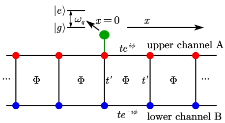
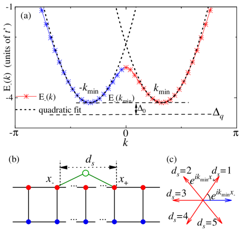
The model of the QED setup we study is depicted in Fig. 1, where a quantum emitter interacts with an artificial one-dimensional waveguide along the direction, which behaves as a photonic analog of the Hofstadter-ladder model. The Hofstadter ladder can be viewed as the two-leg edge of the Harper-Hofstadter model Ozawa et al. (2019), where a synthetic gauge field is applied through each plaquette (see Fig. 1). Here we consider it working as a 1D artificial waveguide which allows photons traveling along it. In this situation, two legs in of the ladder waveguide serve as channel A and B of the waveguide. For convenience, we set the length of one unit site as . The ladder waveguide is composed by two legs, which can be viewed as two quantum channels for the emitter. Two sites in each rung are coupled with strength , which is set as . By adopting a Landau gauge along the direction, the phase connections only appear in each leg. Therefore, the hopping amplitude between two nearest neighbor sites is () for channel A (B). Consequently, by setting , the tight-binding Hamiltonian of the waveguide is Guan et al. (2020)
| (1) | |||||
where () are the annihilation (creation) operators of the sites at position , and is the identical frequency of those bosonic modes. In the following we work in the rotating frame of the constant part .
Under the periodic boundary condition and in the momentum space with
| (2) |
we can diagonalize the waveguide Hamiltonian as
| (5) | |||||
| (6) | |||||
where , and are respectively expressed as
| (7) |
As shown in Eq. (6), the Hamiltonian is expressed in the Pauli operators, indicating that the upper-lower leg degree of freedom behaves as an effective spin. Due to the synthetic gauge field, contains the effective spin-orbit coupling term , which will lead to spin-momentum locking Hügel and Paredes (2014). Note that in condensed matter physics the concept of “spin” is extensively used for models consisting of“A” and “B” sublattices. Similarly, the spin-orbit coupling is a generalized concept from atomic physics, which describes a two-component internal freedom coupling to the momentum of a particle Ozawa et al. (2019). For example, in Refs. Sala et al. (2015); Hafezi et al. (2011), the spin-orbit coupling and spin Hall insulators for photons have been successfully demonstrated in experiments.
The energy spectrum can be derived by simply diagonalizing . Consequently, the energy bands and eigenmodes are derived as
| (8) | |||
| (9) | |||
| (10) |
where . Now we define the average spin as
| (11) |
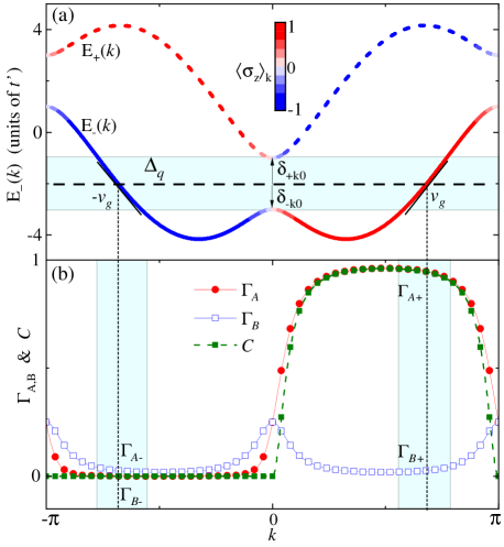
Given that (), the mode asymmetrically distributes on channel () with more probabilities. In Fig. 2(a), we plot and of two bands versus . It is found that, due to spin-momentum locking, the chiral current of the lower band is opposite to the upper band for certain momentum .
Moreover, the spin-orbit coupling significantly modifies the dispersion relation of the waveguide. For a free particle without spin-orbit coupling, the energy minimum point is usually with zero momentum (or ). When spin-orbit coupling appears, the spin-up and spin-down modes minimize their energies by carrying non-zero opposite momentum Galitski and Spielman (2013). As depicted in Fig. 2, the photonic dispersion relation of the ladder waveguide becomes spin-dependent, and the energy minima are degenerate at two points with non-zero momentum . Moreover, there is Kramers degeneracy for a pair of modes due to spin-momentum interaction, and the field distribution is mostly localized in channel A (B) for () Hügel and Paredes (2014). Those properties allow us to realize unconventional phenomena of quantum optics, which will be addressed in the following discussions.
III chiral spontaneous emission
We first consider that the two-energy-level emitter is of small atom form, i.e., couples to the Hofstadter-ladder waveguide at one site (see Fig. 1). Its frequency lies resonantly within the lower energy band. In the rotating frame of bosonic frequency , the system Hamiltonian is written as
| (12) | |||
| (13) |
where with being the emitter’s transition frequency, and , with () being the exited (ground) state of the emitter. Applying inverse Fourier transform, one obtains . According to Eqs. (9, 10), can be decomposed as the superposition of . Finally, the interaction Hamiltonian is written as
| (14) |
As shown in Fig. 2(a), is set in the cyan regime, and only the lower band is resonant with the emitter. To avoid the non-Markovian effects led by the band tops Calajo et al. (2016), we require far away from two band edges, i.e., . By dropping the off-resonant terms with upper band modes , the interacting Hamiltonian is reduced as
| (15) |
After substituting Eq. (9) into Eq. (15), we can divide into two parts which describe interactions with channel A and B respectively:
| (16) | |||
| (17) | |||
| (18) |
From Eq. (16) and as depicted in Fig. 2(a), we find four dissipation terms by assuming the resonant position at , i.e., the left/right direction of channel A (B). After applying the unitary transformation , the interaction operator with channel A becomes
| (19) |
where . Similar to Eq. (19), the interaction operator with channel B can also be written in an integral form. We consider the spontaneous decay process with an excitation initially localized in the emitter. In the single-excitation subspace, the state of the whole system is expressed as , and the evolution of the whole system governed by is derived from the following differential equations
| (20) | |||
| (21) | |||
| (22) |
By substituting the internal form of Eqs. (21, 22) into Eq. (20), the evolution of is derived as
| (23) |
As depicted in Fig. 2(a), we approximate the dispersion relation around to be linear, i.e.,
| (24) | |||||
where is the group velocity at (). By setting , the detuning is written as . In the Born-Markovian regime, the decay rate is required to be much smaller than the band width , and we can extend the integral bound to be infinite. Consequently, Eq. (23) is reduced as
| (25) |
where correspond to the emission rates into the right/left direction of channel , which are derived as
| (26) | |||
| (27) |
which show that are determined by . In this part we only focus on the Markovian decay regime (cyan area in Fig. 2) where both band edges and the upper energy band do not take apparent effects. We plot in Fig. 2(b) [in units of ], and find that the emission to channel A (B) is spatially asymmetric (symmetric), i.e.,
Specially, under the following condition
| (28) |
the emission field mostly distributes on the right side of channel A. Therefore, the spontaneous emission field will chirally propagate along the Hofstadter-ladder waveguide. As discussed in Sec. II, the chirality is led by the effective spin-orbit coupling mechanism.
We assume that the coupling position is at , and therefore, the field intensities on the right (left) side of channel A and B are defined as
| (29) |
where is the field amplitude of site of the rung at of the ladder. For example, if the right side of channel A is the desired direction, both the dissipation into channel B and into the left hand side of channel A will lead to photonic leakage. Consequently, the chiral factor is defined as Lodahl et al. (2017)
| (30) |
By adopting expressions of in Eqs. (26,27), the analytical chiral factor is derived as
| (31) |
where we employ the relation . In Fig. 2(b), we plot chiral factor changing with resonant wave number . Given that , (Note that we have restricted as positive, i.e., ). In this case, , indicating that the field hardly dissipates into the desired channel. When , the chiral factor is simplified as
| (32) |
Therefore, under the condition
| (33) |
most excitation energy will dissipate into the right side of channel A. Those discussions indicate that both the waveguide’s parameters and the resonant position will directly determine the chiral factor.
By adopting the parameters in Fig. 2, we obtain
| (34) |
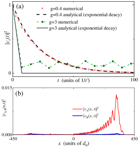
which is a high chiral factor to realize cascaded quantum networks with multiple nodes. To verify our above analysis, in the following we numerically simulate the system’s evolution by adopting the system’s Hamiltonian in Eq. (12). Note that the ladder’s Hamiltonian is expressed in real space [see Eq. (1)], and the ladder length is set as , which is long enough to avoid field reflection by the bounds. Figure 3(a) shows the evolution of the emitter with and , respectively. Given that , the analytical decay rate is calculated as [according to Eqs. (26, 27)], which is much smaller than the band width , and the Markovian approximation is valid. The emitter’s evolution is shown in Fig. 3(a), which decays with time and matches well with the analytical exponential form. In Fig. 3(b), we plot the field distributions at for both channel A and B, where the photonic field mostly distributes on the right side of channel A. By adopting Eq. (29) the numerical chirality is about , which is very close to the analytical result derived in Eq. (34).
Note that all the above results for the chiral decay are derived within the Born-Markovian approximation. When the emitter-waveguide interaction strength is comparable to the band width , both modes around and two energy minima points (see Fig. 2 and Fig. 5) with zero group velocity will prevent the emitter from decaying. Partial excitation energy will be trapped around the coupling position in the form of bound states Calajo et al. (2016). By increasing the emitter-waveguide interaction beyond the Markovian regime with , we plot the emitter’s evolution in Fig. 3(a), which is no longer of exponential decaying form. After dissipating partial energy into the waveguide, the rest is trapped within the emitter. Therefore, to work as a well-performed cascaded quantum system, the emitter in each node should couple to the waveguide within the Markovian regime. Next, we will discuss the behavior of bound states of both small and giant emitters due to band edge effects.
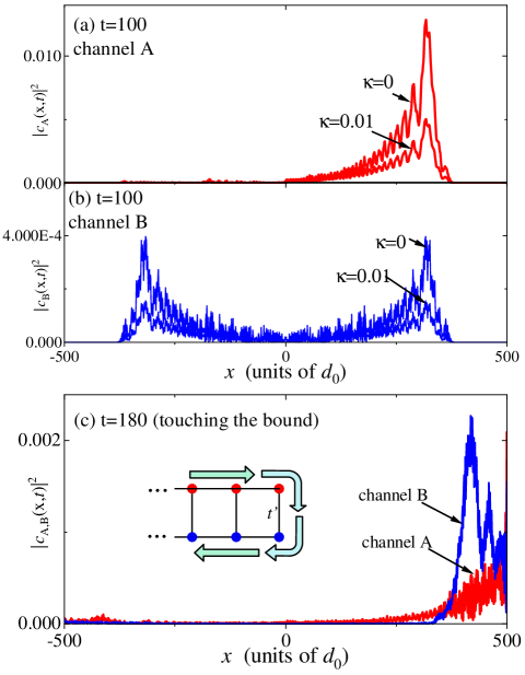
As discussed in experimental work in Refs. Underwood et al. (2012); Houck et al. (2012), the bosonic modes in the Hofstadter-ladder waveguide can be made by cavities or LC resonators, which will experience decoherence led by the noisy environment. The decay of each site is assumed in the Lindblad form, i.e.,
| (35) |
where is the photonic decay rate of each cite. By setting and respectively, we plot the corresponding field distributions along the waveguide at . When the photonic wavepacket propagates along the dissipative waveguide, it will decay the energy into the environment. We find that the amplitude of the photonic field becomes much lower than the non-dissipative case. However, the field distribution is still chiral, which is not affected by this local coherence.
Additionally, in experiments the waveguide’s length cannot be infinite, and therefore, the chiral field will be reflected by the hard-wall boundary of the waveguide after a long-time propagation. In Fig. 4(c), we plot the field distribution at , when the wavepacket already touches the waveguide’s boundary. The energy flow direction is shown in the insets. We find that, due to the hopping rates between two channels at the boundary, most of the energy will be reflected into channel B. Since the photon decay of each rate is also considered, the amplitude of the reflected wavepacket is much lower than that in Fig. 4(a).
IV periodical interference behavior modulated by giant emitter’s size
IV.1 bound state of a single giant emitter
Besides emitting and absorbing real photons, different emitters can also be coherently mediated via exchanging virtual photons in the waveguide, which requires the emitter’s frequency to be outside the spectrum of the waveguide bath Douglas et al. (2016); Bello et al. (2019); Wang et al. (2021a). Here we restrict the frequency detuning below the lower bound of [see Fig. 5(a)]. Additionally, the emitter is assumed to be of giant atom form Kockum et al. (2014); Guo et al. (2017); Kockum et al. (2018); Kockum (2020); Kannan et al. (2020); Zhao and Wang (2020); Du et al. (2021); Zhang et al. (2021); Wang et al. (2021b); Du et al. (2022), which couples to the waveguide at two points of channel A (or B), as depicted in Fig. 5(b). The separation distance is denoted as , which corresponds to the giant emitter’s size. Similar to previous discussions, the interaction strengths with channel A and B [see Eqs. (17,18)] are written as
| (36) | |||
| (37) |
where is the interaction strength with a single point. Note that under the condition , two coupling positions coincide at the same site, and the giant atom degrades as a small atom.
Similar to Eqs. (20-22), we can obtain differential equations for and . Defining , the evolution is derived in Laplace space with and Calajo et al. (2016); Bello et al. (2019); Wang and Li (2022)
| (38) | |||
| (39) |
Consequently, is obtained as
| (40) |
By substituting Eq. (40) into Eq. (38), is derived as
| (41) | |||
| (42) |
where is the self-energy. The time-dependent evolution is recovered from the inverse Laplace transform Ramos et al. (2016)
| (43) |
Given that the waveguide is long enough to avoid reflection effects, we can write the self-energy in the integral form by replacing with . Substituting the relations
| (44) | |||
| (45) |
into Eq. (42), the self-energy is expressed as
| (46) |
where .
Due to the effective spin-orbit coupling, the energy minimum point is split into two with non-zero momentum . At the positions of two dips, the group velocities are zero, which can be derived from Eq. (24)
| (47) |
Therefore, their positions are derived as
| (48) |
At , the second-order derivatives are non-zero, and we denote the curvature as
| (49) |
As depicted in Fig. 5(a), we employ the effective mass approximation, to fit the dispersion around the band edges with quadratic relations
| (50) |
By substituting Eq. (50) into Eq. (46), the self-energy is calculated as
| (51) | |||||
where is the detuning to the band edge [see Fig. 5(a)]. We assume that is small, and therefore, only the modes around contribute significantly to . Consequently, we can approximate
| (52) |
and extend the integral bound of Eq. (51) to be infinite. Finally, we obtain
| (53) |
where we have employed the following relations
| (54) |
In this work, the adopted parameters of the waveguide satisfy
| (55) |
As shown in Fig. 5(c), the phase relation between two coupling points will rotate counter-clockwise when increasing giant emitter’s size (). Therefore, the relative phase between is very essential for the dynamics of the giant emitter. The interference between two points is maximum destructive (constructive) given that (). When is much stronger than , most energy will be trapped in the emitter in the form of the bound state Calajo et al. (2016); González-Tudela and Cirac (2017); Wang and Li (2022). The trapped excitation probability is determined by the pure imaginary pole of the following transcendental equation Wang and Li (2022)
| (56) |
and the steady state population of the emitter is derived via the residue theorem Calajo et al. (2016)
| (57) | |||
| (58) |
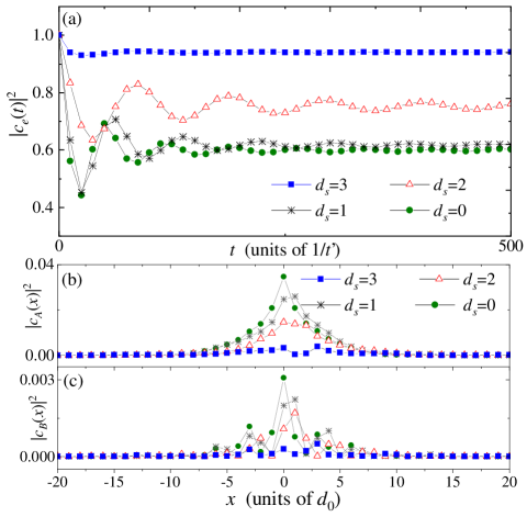
In Fig. 6(a), we plot dynamical evolutions of for different giant emitter’s sizes . When (a small emitter), the effective interacting strength is strongest, which is enhanced by the constructive interference between two coupling legs. The steady state reaches lowest, and the emitter can effectively distribute its energy into the waveguide. That is, the photonic bound state is mostly localized in channel A due to the relation
| (59) |
which can be seen clearly by comparing Fig. 6(b) and Fig. 6(c).
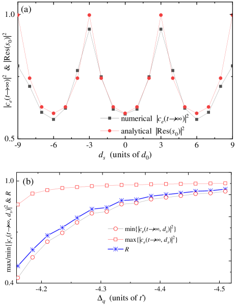
When increasing the distance between two coupling points, the constructive interference will be reversed as destructive, with being significantly weaken. When , the phase difference satisfies , indicating that the interaction strength is approximately zero, i.e., [see Fig. 5(c)]. The giant emitter approximately decouples with the waveguide. Due to this decoupling mechanism, the excitation trapped in the emitter reaches its maximum, as shown in Fig. 6(a). Figure 6(b, c) show that the destructive interference will also suppress the bound state’s amplitude significantly. We plot the steady state population changing with in Fig. 7(a), which clearly presents a periodical interference pattern of modulated by the giant atom’s size. Note that we only take for example. Note that The periodical length is tunable by controlling the parameters of the Hofstadter ladder waveguide. By adopting another according Eq. (48), different spatial interference patterns can also be observed. The oscillating pattern in Fig. 7(a) is due to interference between different points in the giant atom, and the peaks (dips) correspond to the positions where the maximum constructive (destructive) interference happens. Therefore, we can define the contrast ratio for the interference as
| (60) |
For the parameters employed in Fig. 7(a), () is located at (), which corresponds to a small (giant) atom. A smaller indicates that the dynamical difference between small and giant atoms is more apparent. In Fig. 7(b), we plot maximum/minimum and changing with the frequency detuning . When shifting away from the band edge, the contributions of the band-edge modes to the bound states will be significantly suppressed. Therefore, a larger will reduce the interference effects, which corresponds to [see Fig. 7(b)]. To observe better interference effect in experiments, the emitter frequency can be close to the edge of the lower energy band.
IV.2 dipole-dipole interactions
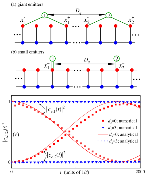
By exchanging virtual photons in the waveguide, between emitters there are long-range dipole-dipole interactions which are determined by the overlap areas between their bound states González-Tudela et al. (2015); Douglas et al. (2016); Bello et al. (2019). As shown in Fig. 8(a, b), we now discuss the multiple emitters interacting with the same ladder waveguide. Due to the interference mechanism presented above, we focus on revealing the relation between giant emitter’s size and the quantum dynamics where dipole-dipole interactions are involved.
Both two giant emitters are assumed to couple with channel A, and the coupling topology is of separation form Kockum et al. (2018). Similar to the single emitter case, the interaction Hamiltonian is written as
| (61) |
where is the coupling strength between emitter and the waveguide. We consider two emitters with identical frequency which is also below the lower bound of . To proceed, we define the average distance between two emitters as
| (62) |
The dipole-dipole interaction can be tediously derived via the standard resolvent-operator techniques González-Tudela et al. (2015); Douglas et al. (2016); Bello et al. (2019); Wang et al. (2021a). However, given that the detuning is large and the waveguide is only virtually excited, corresponds to the effective coupling strength mediated by the waveguide’s modes, which can be simply derived via the effective Hamiltonian methods James and Jerke (2007). In the rotating frame of free energies of both emitters and waveguide, we first write in Eq. (61) in the time-dependent form
| (63) |
where . We first calculate the coupling rate mediated by one mode . By employing the methods in Ref. [76], the one-mode-mediated effective Hamiltonian is derived as
| (64) | |||||
Since the waveguide is only virtually excited and approximately in its vacuum state, we can trace off the freedom of mode by adopting the following approximation
| (65) |
Consequently, is simplified as
| (66) |
Note that is mediated by one mode, and the total dipole-dipole interaction should take all the modes’ contribution into account. Consequently, the total dipole-dipole interaction Hamiltonian mediated by all the waveguide’s modes is derived as
| (67) |
where is the total interaction strength which is written as
| (68) | |||||
Since the emitter frequency is below the edge of the lower energy band [see Fig. 5(a)], the dispersion relation can be fit with the quadratic relations in Eq. (50). Without loss of generality, we set since only relative distance matters. As depicted in Fig. 8(a), two emitters are separated with a distance . Given that , can be written as
| (69) | |||||
As shown in Eq. (26) and depicted in Fig. 2(b), the following relation
is valid for the parameters employed in this work. Consequently, we can neglect the first part () in Eq. (69), and is derived as
| (70) |
which indicates that that dipole-dipole interactions are determined by the overlap areas between two bound states of emitters González-Tudela et al. (2015). Similar to the process obtaining the self-energy in Eqs. (51, 53), we derive as
| (71) |
which shows that exponentially decays with emitters’ separation distance. Similar results have been obtained in Refs. González-Tudela et al. (2015); Douglas et al. (2016); Wang et al. (2021a).
As shown in Fig. 7(b, c), the amplitude of the bound state will periodically change with due to the interference effect. When , the photonic bound state approximately disappears. Consequently, the overlapping area is also nearly zero. By assuming the initial excitation being in emitter 1, we numerically plot the Rabi oscillations between giant emitters () and small emitters () in Fig. 8(c), respectively. We find that, due to the destructive interference, when , two emitters hardly exchange energy, and decouple with each other (). On the contrary, two emitters will exchange excitation rapidly at a large rate due to the constructive interference when is reduced to be zero.
V Conclusion and outlooks
In this work, we explore the unconventional quantum optics by considering a Hofstadter-ladder waveguide interacting with both small and giant emitters. Due to the effective spin-orbit coupling, both the waveguide’s vacuum modes and spectrum show nontrivial properties. In the first part, we consider a small emitter which frequency is resonant with one energy band. Two legs of the ladder, which can be viewed as the freedoms in an effective spin locked with the momemtum freedom, provide two dissipating channels. The spontaneous emission is chiral with most photonic field decaying unidirectionally. Both numerical and analytical results show that the Hofstadter-ladder waveguide can work as a well-performed quantum bus of a chiral network.
In the second part, the emitters are assumed of giant atom form with frequencies below the lower energy band. In this scenario, only the modes around two energy minima points induced by the spin-orbit coupling contribute significantly to the system’s dynamics, which will lead to emitter-waveguide bound states. Since the energy minima modes carry non-zero momentum, the coupling strengths are periodically modulated by the giant emitter’s size due to quantum interference. Specially the giant emitter will decouple with the waveguide when maximum destructive interference happens. This mechanism provides a novel approach to control long-range dipole-dipole interactions between emitters by modulating their sizes.
In this work, the giant emitter is assumed to couple with the sites of the same channel. Other intriguing effects might be observed by considering the coupling points on different channels. Moreover, for multiple giant emitters, we just consider the coupling points arranged in the sepration form. In fact there are some other distinct topologies, which are nested and braided cases Kockum et al. (2018). Exploring the coupling topology effects might also bring novel quantum phenomena. There are already plenty of work about realizing artificial Hofstadter ladders in various quantum systems such as cold atoms and circuit-QED Tai et al. (2017); Gu et al. (2017); Guan et al. (2020); Weitenberg and Simonet (2021), which can be potential platforms to demonstrate above unconventional QED phenomena. We hope that our work will open the possibilities of exploring novel quantum effects in artificial spin-orbit-coupling environments.
VI Acknowledgments
The quantum dynamical simulations are based on open source code QuTiP Johansson et al. (2012, 2013). X.W. is supported by the National Natural Science Foundation of China (NSFC) (Grant No. 12174303 and No. 11804270), and China Postdoctoral Science Foundation No. 2018M631136. H.R.L. is supported by the National Natural Science Foundation of China (NSFC) (Grant No.11774284).
References
- Cohen-Tannoudji et al. (1998) C. Cohen-Tannoudji, J. Dupont-Roc, and G. Grynberg, Atom–Photon Interactions (Wiley, 1998).
- Clerk et al. (2010) A. A. Clerk, M. H. Devoret, S. M. Girvin, F. Marquardt, and R. J. Schoelkopf, “Introduction to quantum noise, measurement, and amplification,” Rev. Mod. Phys. 82, 1155 (2010).
- Lamb and Retherford (1947) W. E. Lamb and R. C. Retherford, “Fine structure of the hydrogen atom by a microwave method,” Phys. Rev. 72, 241 (1947).
- Scully and Zubairy (1997) Marlan O. Scully and M. Suhail Zubairy, Quantum Optics (Cambridge University Press, 1997).
- John and Quang (1994) S. John and T. Quang, “Spontaneous emission near the edge of a photonic band gap,” Phys. Rev. A 50, 1764 (1994).
- Lambropoulos et al. (2000) P. Lambropoulos, G. M. Nikolopoulos, T. R. Nielsen, and S. Bay, “Fundamental quantum optics in structured reservoirs,” Rep. Prog. Phys. 63, 455 (2000).
- Giraldi and Petruccione (2011) F. Giraldi and F. Petruccione, “Reservoir for inverse-power-law decoherence of a qubit,” Phys. Rev. A 83, 012107 (2011).
- Lodahl et al. (2015) P. Lodahl, S. Mahmoodian, and S. Stobbe, “Interfacing single photons and single quantum dots with photonic nanostructures,” Rev. Mod. Phys. 87, 347 (2015).
- Stewart et al. (2020) M. Stewart, J. Kwon, A. Lanuza, and D. Schneble, “Dynamics of matter-wave quantum emitters in a structured vacuum,” Phys. Rev. Research 2, 043307 (2020).
- Ferreira et al. (2021) V. S. Ferreira, J. Banker, A. Sipahigil, M. H. Matheny, A. J. Keller, E. Kim, M. Mirhosseini, and O. Painter, “Collapse and revival of an artificial atom coupled to a structured photonic reservoir,” Phys. Rev. X 11, 041043 (2021).
- Petersen et al. (2014) J. Petersen, J. Volz, and A. Rauschenbeutel, “Chiral nanophotonic waveguide interface based on spin-orbit interaction of light,” Science 346, 67 (2014).
- Bliokh and Nori (2015) K. Y. Bliokh and F. Nori, “Transverse and longitudinal angular momenta of light,” Phys. Rep. 592, 1 (2015).
- Bliokh et al. (2015) K. Y. Bliokh, F. J. Rodríguez-Fortuño, F. Nori, and A. V. Zayats, “Spin–orbit interactions of light,” Nature Photon. 9, 796 (2015).
- Lodahl et al. (2017) P. Lodahl, S. Mahmoodian, S. Stobbe, A. Rauschenbeutel, P. Schneeweiss, J. Volz, H. Pichler, and P. Zoller, “Chiral quantum optics,” Nature (London) 541, 473 (2017).
- Lang et al. (2022) B. Lang, D. P. S. McCutcheon, E. Harbord, A. B. Young, and R. Oulton, “Perfect chirality with imperfect polarization,” Phys. Rev. Lett. 128, 073602 (2022).
- John and Wang (1990) S. John and J. Wang, “Quantum electrodynamics near a photonic band gap: Photon bound states and dressed atoms,” Phys. Rev. Lett. 64, 2418 (1990).
- Goban et al. (2014) A. Goban, C.-L. Hung, S.-P. Yu, J.D. Hood, J.A. Muniz, J.H. Lee, M.J. Martin, A.C. McClung, K.S. Choi, D.E. Chang, O. Painter, and H.J. Kimble, “Atom–light interactions in photonic crystals,” Nat. Commun. 5, 4808 (2014).
- González-Tudela et al. (2015) A. González-Tudela, C.-L. Hung, D. E. Chang, J. I. Cirac, and H. J. Kimble, “Subwavelength vacuum lattices and atom–atom interactions in two-dimensional photonic crystals,” Nature Photon. 9, 320 (2015).
- Douglas et al. (2016) J. S. Douglas, T. Caneva, and D. E. Chang, “Photon molecules in atomic gases trapped near photonic crystal waveguides,” Phys. Rev. X 6, 031017 (2016).
- Liu and Houck (2017) Y. B. Liu and A. A. Houck, “Quantum electrodynamics near a photonic bandgap,” Nat. Phys. 13, 48 (2017).
- Chang et al. (2018) D. E. Chang, J. S. Douglas, A. González-Tudela, C.-L. Hung, and H. J. Kimble, “Colloquium: Quantum matter built from nanoscopic lattices of atoms and photons,” Rev. Mod. Phys. 90, 031002 (2018).
- Wang et al. (2021a) X. Wang, T. Liu, A. F. Kockum, H.-R. Li, and F. Nori, “Tunable chiral bound states with giant atoms,” Phys. Rev. Lett. 126, 043602 (2021a).
- Douglas et al. (2015) J. S. Douglas, H. Habibian, C.-L. Hung, A. V. Gorshkov, H. J. Kimble, and D. E. Chang, “Quantum many-body models with cold atoms coupled to photonic crystals,” Nature Photon. 9, 326 (2015).
- Shahmoon and Kurizki (2013) E. Shahmoon and G. Kurizki, “Nonradiative interaction and entanglement between distant atoms,” Phys. Rev. A 87, 033831 (2013).
- Ying et al. (2019) L. Ying, M. Zhou, M. Mattei, B.-Y. Liu, P. Campagnola, R. H. Goldsmith, and Z.-F. Yu, “Extended range of dipole-dipole interactions in periodically structured photonic media,” Phys. Rev. Lett. 123, 173901 (2019).
- Ramos et al. (2016) T. Ramos, B. Vermersch, P. Hauke, H. Pichler, and P. Zoller, “Non-markovian dynamics in chiral quantum networks with spins and photons,” Phys. Rev. A 93, 062104 (2016).
- Calajo et al. (2016) G. Calajo, F. Ciccarello, D. Chang, and P. Rabl, “Atom-field dressed states in slow-light waveguide QED,” Phys. Rev. A 93, 033833 (2016).
- González-Tudela and Cirac (2018) A. González-Tudela and J. I. Cirac, “Exotic quantum dynamics and purely long-range coherent interactions in dirac conelike baths,” Phys. Rev. A 97, 043831 (2018).
- González-Tudela et al. (2019) A. González-Tudela, C. S. Muñoz, and J. I. Cirac, “Engineering and harnessing giant atoms in high-dimensional baths: A proposal for implementation with cold atoms,” Phys. Rev. Lett. 122, 203603 (2019).
- Leonforte et al. (2021) L. Leonforte, A. Carollo, and F. Ciccarello, “Vacancy-like dressed states in topological waveguide qed,” Phys. Rev. Lett. 126, 063601 (2021).
- González-Tudela and Cirac (2017) A. González-Tudela and J. I. Cirac, “Markovian and non-markovian dynamics of quantum emitters coupled to two-dimensional structured reservoirs,” Phys. Rev. A 96, 043811 (2017).
- González-Tudela and Cirac (2017) A. González-Tudela and J. I. Cirac, “Quantum emitters in two-dimensional structured reservoirs in the nonperturbative regime,” Phys. Rev. Lett. 119, 143602 (2017).
- Bello et al. (2019) M. Bello, G. Platero, J. I. Cirac, and A. González-Tudela, “Unconventional quantum optics in topological waveguide QED,” Sci. Adv. 5, eaaw0297 (2019).
- Kim et al. (2021) E. Kim, X. Zhang, V. S. Ferreira, J. Banker, J. K. Iverson, A. Sipahigil, M. Bello, A. González-Tudela, Mo. Mirhosseini, and O. Painter, “Quantum electrodynamics in a topological waveguide,” Phys. Rev. X 11, 011015 (2021).
- Roccati et al. (2022) F. Roccati, S. Lorenzo, G. Calajò, G. M. Palma, A. Carollo, and F. Ciccarello, “Exotic interactions mediated by a non-hermitian photonic bath,” Optica 9, 565–571 (2022).
- Gong et al. (2022) Z. Gong, M. Bello, D. Malz, and F. K. Kunst, “Bound states and photon emission in non-hermitian nanophotonics,” preprint arXiv:2205.05490 (2022).
- Zhang (2000) S.-F. Zhang, “Spin hall effect in the presence of spin diffusion,” Phys. Rev. Lett. 85 (2000), 10.1103/PHYSREVLETT.85.393.
- Murakami et al. (2003) S. Murakami, N. Nagaosa, and S.-C. Zhang, “Dissipationless quantum spin current at room temperature,” Science 301, 1348 (2003).
- Sinova et al. (2004) J. Sinova, D. Culcer, Q. Niu, N. A. Sinitsyn, T. Jungwirth, and A. H. MacDonald, “Universal intrinsic spin hall effect,” Phys. Rev. Lett. 92, 126603 (2004).
- Wunderlich et al. (2005) J. Wunderlich, B. Kaestner, J. Sinova, and T. Jungwirth, “Experimental observation of the spin-hall effect in a two-dimensional spin-orbit coupled semiconductor system,” Phys. Rev. Lett. 94, 047204 (2005).
- Kane and Mele (2005) C. L. Kane and E. J. Mele, “Quantum spin hall effect in graphene,” Phys. Rev. Lett. 95, 226801 (2005).
- Galitski and Spielman (2013) V. Galitski and I. B. Spielman, “Spin–orbit coupling in quantum gases,” Nature (London) 494, 49 (2013).
- Zhou et al. (2013) X.-F. Zhou, Y. Li, Z. Cai, and C.J. Wu, “Unconventional states of bosons with the synthetic spin–orbit coupling,” J. Phys. B: At., Mol. Opt. Phys. 46, 134001 (2013).
- Wu et al. (2016) Z. Wu, L. Zhang, W. Sun, X.-T. Xu, B.-Z. Wang, S.-C. Ji, Y.-J. Deng, S. Chen, X.-J. Liu, and J.-W. Pan, “Realization of two-dimensional spin-orbit coupling for bose-einstein condensates,” Science 354, 83 (2016).
- Kartashov et al. (2017) Y. V. Kartashov, V. V. Konotop, and L. Torner, “Bound states in the continuum in spin-orbit-coupled atomic systems,” Phys. Rev. A 96, 033619 (2017).
- Livi et al. (2016) L. F. Livi, G. Cappellini, M. Diem, L. Franchi, C. Clivati, M. Frittelli, F. Levi, D. Calonico, J. Catani, M. Inguscio, and L. Fallani, “Synthetic dimensions and spin-orbit coupling with an optical clock transition,” Phys. Rev. Lett. 117, 220401 (2016).
- Liu et al. (2011) L.-Q. Liu, T. Moriyama, D. C. Ralph, and R. A. Buhrman, “Spin-torque ferromagnetic resonance induced by the spin hall effect,” Phys. Rev. Lett. 106 (2011), 10.1103/PhysRevLett.106.036601.
- Sala et al. (2015) V. G. Sala, D. D. Solnyshkov, I. Carusotto, T. Jacqmin, A. Lemaître, H. Terças, A. Nalitov, M. Abbarchi, E. Galopin, I. Sagnes, J. Bloch, G. Malpuech, and A. Amo, “Spin-orbit coupling for photons and polaritons in microstructures,” Phys. Rev. X 5, 011034 (2015).
- Salerno et al. (2017) G. Salerno, A. Berardo, T. Ozawa, H. M. Price, L. Taxis, N. M. Pugno, and I. Carusotto, “Spin–orbit coupling in a hexagonal ring of pendula,” New J. Phys. 19, 055001 (2017).
- Creutz (2001) M. Creutz, “Aspects of chiral symmetry and the lattice,” Rev. Mod. Phys. 73, 119 (2001).
- Narozhny et al. (2005) B. N. Narozhny, S. T. Carr, and A. A. Nersesyan, “Fractional charge excitations in fermionic ladders,” Phys. Rev. B 71, 161101 (2005).
- Jaefari and Fradkin (2012) A. Jaefari and E. Fradkin, “Pair-density-wave superconducting order in two-leg ladders,” Phys. Rev. B 85, 035104 (2012).
- Atala et al. (2014) M. Atala, M. Aidelsburger, M. Lohse, J. T. Barreiro, B. Paredes, and I. Bloch, “Observation of chiral currents with ultracold atoms in bosonic ladders,” Nature Physics 10, 588 (2014).
- Tai et al. (2017) M. E. Tai, A. Lukin, M. Rispoli, R. Schittko, T. Menke, D. Borgnia, P. M. Preiss, F. Grusdt, A. M. Kaufman, and M. Greiner, “Microscopy of the interacting Harper–hofstadter model in the two-body limit,” Nature (London) 546, 519–523 (2017).
- Yuan et al. (2019) L.-Q. Yuan, Q. Lin, A.-W. Zhang, M. Xiao, X.-F. Chen, and S.H. Fan, “Photonic gauge potential in one cavity with synthetic frequency and orbital angular momentum dimensions,” Phys. Rev. Lett. 122, 083903 (2019).
- Guan et al. (2020) X. Guan, Y.-L. Feng, Z.-Y. Xue, G. Chen, and S.T. Jia, “Synthetic gauge field and chiral physics on two-leg superconducting circuits,” Phys. Rev. A 102, 032610 (2020).
- Hügel and Paredes (2014) D. Hügel and B. Paredes, “Chiral ladders and the edges of quantum hall insulators,” Phys. Rev. A 89, 023619 (2014).
- Sánchez-Burillo et al. (2020) E. Sánchez-Burillo, C. Wan, D. Zueco, and A. González-Tudela, “Chiral quantum optics in photonic sawtooth lattices,” Phys. Rev. Research 2, 023003 (2020).
- Wang et al. (2020) X. Wang, H.-R. Li, and F.-L. Li, “Generating synthetic magnetism via floquet engineering auxiliary qubits in phonon-cavity-based lattice,” New J. Phys. 22, 033037 (2020).
- De Bernardis et al. (2021) D. De Bernardis, Z.-P. Cian, I. Carusotto, M. Hafezi, and P. Rabl, “Light-matter interactions in synthetic magnetic fields: Landau-photon polaritons,” Phys. Rev. Lett. 126, 103603 (2021).
- Dong et al. (2021) X.-L. Dong, P.-B. Li, T. Liu, and F. Nori, “Unconventional quantum sound-matter interactions in spin-optomechanical-crystal hybrid systems,” Phys. Rev. Lett. 126, 203601 (2021).
- Mittal et al. (2014) S. Mittal, J. Fan, S. Faez, A. Migdall, J. M. Taylor, and M. Hafezi, “Topologically robust transport of photons in a synthetic gauge field,” Phys. Rev. Lett. 113, 087403 (2014).
- Calajó et al. (2019) G. Calajó, M. J. A. Schuetz, H. Pichler, M. D. Lukin, P. Schneeweiss, J. Volz, and P. Rabl, “Quantum acousto-optic control of light-matter interactions in nanophotonic networks,” Phys. Rev. A 99, 053852 (2019).
- Gheeraert et al. (2020) N. Gheeraert, S. Kono, and Y. Nakamura, “Programmable directional emitter and receiver of itinerant microwave photons in a waveguide,” Phys. Rev. A 102, 053720 (2020).
- Wang et al. (2022) X. Wang, Y.-F. Lin, J.-Q. Li, W.-X. Liu, and H.-R. Li, “Chiral SQUID-metamaterial waveguide for circuit-QED,” preprint arXiv:2206.06579 (2022).
- Solano et al. (2021) P. Solano, P. Barberis-Blostein, and K. Sinha, “Dissimilar collective decay and directional emission from two quantum emitters,” preprint arXiv:2108.12951 (2021).
- Kannan et al. (2022) B. Kannan, A. Almanakly, Y. Sung, A. D. Paolo, D. A. Rower, J. Braumüller, A. Melville, B. M. Niedzielski, A. Karamlou, and K. Serniak, “On-demand directional photon emission using waveguide quantum electrodynamics,” preprint arXiv:2203.01430 (2022).
- Kockum et al. (2014) A. F. Kockum, P. Delsing, and G. Johansson, “Designing frequency-dependent relaxation rates and Lamb shifts for a giant artificial atom,” Phys. Rev. A 90, 013837 (2014).
- Guo et al. (2017) L.-Z. Guo, A. Grimsmo, A. F. Kockum, M. Pletyukhov, and G. Johansson, “Giant acoustic atom: A single quantum system with a deterministic time delay,” Phys. Rev. A 95, 053821 (2017).
- Kockum et al. (2018) A. F. Kockum, G. Johansson, and F. Nori, “Decoherence-free interaction between giant atoms in waveguide quantum electrodynamics,” Phys. Rev. Lett. 120, 140404 (2018).
- Kockum (2020) A. F. Kockum, “Quantum optics with giant atoms—the first five years,” International Symposium on Mathematics, Quantum Theory, and Cryptography, , 125 (2020).
- Kannan et al. (2020) B. Kannan, M. J. Ruckriegel, D. L. Campbell, A. F. Kockum, J. Braumüller, D. K. Kim, M. Kjaergaard, P. Krantz, A. Melville, B. M. Niedzielski, A. Vepsäläinen, R. Winik, J. L. Yoder, F. Nori, T. P. Orlando, S. Gustavsson, and W. D. Oliver, “Waveguide quantum electrodynamics with superconducting artificial giant atoms,” Nature (London) 583, 775 (2020).
- Zhao and Wang (2020) W. Zhao and Z. Wang, “Single-photon scattering and bound states in an atom-waveguide system with two or multiple coupling points,” Phys. Rev. A 101, 053855 (2020).
- Du et al. (2021) L. Du, Y.-T. Chen, and Y. Li, “Nonreciprocal frequency conversion with chiral -type atoms,” Phys. Rev. Research 3, 043226 (2021).
- Zhang et al. (2021) Y.-X. Zhang, C. Carceller, M. Kjaergaard, and A. S. Sørensen, “Charge-noise insensitive chiral photonic interface for waveguide circuit QED,” Phys. Rev. Lett. 127, 233601 (2021).
- Wang et al. (2021b) C. Wang, X.-S. Ma, and M.-T. Cheng, “Giant atom-mediated single photon routing between two waveguides,” Opt. Express 29, 40116 (2021b).
- Du et al. (2022) L. Du, Y.-T. Chen, Y. Zhang, and Y. Li, “Giant atoms with time-dependent couplings,” preprint arXiv:2201.12575 (2022).
- Guo et al. (2020) L.-Z. Guo, A. F. Kockum, F. Marquardt, and G. Johansson, “Oscillating bound states for a giant atom,” Phys. Rev. Research 2, 043014 (2020).
- Ozawa et al. (2019) T. Ozawa, H. M. Price, A. Amo, N. Goldman, M. Hafezi, L. Lu, M. C. Rechtsman, D. Schuster, J. Simon, O. Zilberberg, and I. Carusotto, “Topological photonics,” Rev. Mod. Phys. 91, 015006 (2019).
- Hafezi et al. (2011) M. Hafezi, E. A. Demler, M. D. Lukin, and J. M. Taylor, “Robust optical delay lines with topological protection,” Nat. Phys. 7, 907–912 (2011).
- Underwood et al. (2012) D. L. Underwood, W. E. Shanks, Jens Koch, and A. A. Houck, “Low-disorder microwave cavity lattices for quantum simulation with photons,” Phys. Rev. A 86, 023837 (2012).
- Houck et al. (2012) A. A. Houck, H. E., and J. Koch, “On-chip quantum simulation with superconducting circuits,” Nature Physics 8, 292–299 (2012).
- Wang and Li (2022) X. Wang and H.-R. Li, “Chiral quantum network with giant atoms,” Quantum Sci. Technol. 7, 035007 (2022).
- James and Jerke (2007) D. F. James and J. Jerke, “Effective hamiltonian theory and its applications in quantum information,” Can. J. Phys. 85, 625 (2007).
- Gu et al. (2017) X. Gu, A. F. Kockum, A. Miranowicz, Y.-X. Liu, and F. Nori, “Microwave photonics with superconducting quantum circuits,” Phys. Rep. 718-719, 1 (2017).
- Weitenberg and Simonet (2021) C. Weitenberg and J. Simonet, “Tailoring quantum gases by floquet engineering,” Nat. Phys. 17, 1342–1348 (2021).
- Johansson et al. (2012) J. R. Johansson, P. D. Nation, and F. Nori, “Qutip: An open-source Python framework for the dynamics of open quantum systems,” Comput. Phys. Commun. 183, 1760 (2012).
- Johansson et al. (2013) J. R. Johansson, P. D. Nation, and F. Nori, “Qutip 2: A Python framework for the dynamics of open quantum systems,” Comput. Phys. Commun. 184, 1234 (2013).