Unconditionally optimal error estimate of a linearized variable-time-step BDF2 scheme for nonlinear parabolic equations
Abstract
In this paper we consider a linearized variable-time-step two-step backward differentiation formula (BDF2) scheme for solving nonlinear parabolic equations. The scheme is constructed by using the variable time-step BDF2 for the linear term and a Newton linearized method for the nonlinear term in time combining with a Galerkin finite element method (FEM) in space. We prove the unconditionally optimal error estimate of the proposed scheme under mild restrictions on the ratio of adjacent time-steps, i.e. and on the maximum time step. The proof involves the discrete orthogonal convolution (DOC) and discrete complementary convolution (DCC) kernels, and the error splitting approach. In addition, our analysis also shows that the first level solution obtained by BDF1 (i.e. backward Euler scheme) does not cause the loss of global accuracy of second order. Numerical examples are provided to demonstrate our theoretical results.
keywords: two-step backward differentiation formula; the discrete orthogonal convolution kernels; the discrete complementary convolution kernels; error estimates; variable time-step; Unconditional error estimate; error splitting approach
1 Introduction
In this paper, we focus on the unconditionally optimal error estimate of a linearized second-order two-step backward differentiation formula (BDF2) scheme with variable time steps for solving the following general nonlinear parabolic equation [4, 21]:
| (1.1) | ||||||
where is a bounded convex domain. To construct variable time-step schemes, we first set the variable time levels , the th time-step size , the maximum step size , and the adjacent time-step ratios Set , and denote by the approximation of the exact solution . The first step value is calculated by one-step backward difference formula (BDF1), and the other is calculated by BDF2 formula with variable time steps, which are respectively given as
| (1.2) |
The nonlinear term is approximated by a linearized method, i.e., the Newton linearized method given as
| (1.3) |
Thus the semi-discrete BDF2 scheme with variable time steps to problem (1.1) is given as
| (1.4) | |||||
| (1.5) | |||||
| (1.6) |
Here the BDF1 and BDF2 formulas have been written as a unified convolution form of
| (1.7) |
by taking
For the spatial discretization, let be the quasiuniform partition of with triangles in or tetrahedra in , see [11, 19]. Denote the spatial mesh size by and the finite-dimensional subspace of by which consists of piecewise polynomials of degree on . Then, the Newton linearized Galerkin FEM BDF2 scheme with variable time steps is to find such that
| (1.8) |
Efficiency, accuracy and reliability are of key considerations in numerical analysis and scientific computing. For the time-dependent models appeared in science and engineering, a heuristic and promising method to improve efficiency without sacrificing accuracy is the time adaptive method. For instance, one may employ the coarse-grained or refined time steps based on the solutions changing slowly or rapidly to capture the dynamics of the solutions. Another alternative approach is to employ high-order methods in time to have the same accuracy with a relatively large time-step. In this paper, we consider the second order BDF2 scheme with variable time steps.
Due to its nice property (-stable), the BDF2 method with variable time steps has been widely used in various models to obtain computationally efficient, accurate results [2, 23, 20, 16, 15, 13]. Much works have been carried out on its stability and error estimates [22, 17, 5, 3, 2, 1], but the analysis even for linear parabolic problems (i.e., problem (1.1) with ) is already highly nontrivial and challenging as documented in the classic book [19, Chapter 10]. One also refers to the details in [6, 7, 5, 8, 18]. In particular, with the energy method and under a ratio condition , Becker [1] presents that the variable time-step BDF2 scheme for a linear parabolic problems is zero-stable. After that, Emmrich [3] gives the similar result with . Recently, a promising work in [2] introduce a novel generalized discrete Grönwall-type inequality for the Cahn-Hilliard equation to obtain an energy stability with . The works in [17, 22] consider linear parabolic equations based on DOC kernels under [17] and [22], respectively. In addition, the robust second-order convergence is further analyzed in [22]. The robustness here means the optimal second-order accuracy holds valid only requiring the time-step sizes .
For the variable-time-step BDF2 method applied to nonlinear parabolic equations, there has a great progress on the error estimates for the Cahn-Hilliard equation [2], molecular beam epitaxial model without slope selection [23, 15], phase field crystal model [13], and references therein. Among all the numerical methods in [2, 23, 15, 13], the implicit schemes are utlized to deal with the nonlinear terms. Although the implicit schemes are unconditionally stable, they need to solve a nonlinear algebraic system in each time level. To circumvent the extra computational cost for iteratively solving the nonlinear algebraic system, a popular approach is to employ the linearized methods to approximate the nonlinear terms. Combining the variable-time-step BDF2 for linear terms with a linearized method for nonlinear terms, it is natural to ask if the proposed implicit-explicit schemes still remain unconditionally stable. In addition, the focus of this paper is on the general nonlinearity , which also brings the extra analysis difficulty comparing with the phase-fields models studied in [2, 23, 15, 13], since the good property of the energy dissipation for the phase-fields models does not hold any more for general nonlinearity.
In this paper, we aim to address the unconditionally optimal error estimate of the linearized scheme (1.8) in the sense of -norm under the following two conditions:
-
A1 :
for any small constant and , where is the root of equation ;
-
A2 :
there exists a constant independent of and such that the maximum time step size satisfies .
The proof of the error estimate is established by the introduction of the temporal-spatial error splitting approach and the concepts of DOC and DCC kernels. The error splitting approach, developed in [9], is used to overcome the unnecessary restrictions of the temporal and spacial mesh sizes. The main idea of the error splitting approach is to first consider the boundedness of for the solution to semi-discrete equation (1.4), and then to obtain the estimate of for the fully discrete equation (1.8) by using the following strategy
| (1.9) | ||||
where is the projection operator.
The concepts of DOC and DCC kernels, developed in [17, 22], are used to present the stability and convergence analysis under a mild restriction on the ratio of adjacent time-steps, i.e., A1. The condition A1 is the mildest restriction in the current literatures, as far as we know, for the variable time-step BDF2 method. On the other hand, due to the usage of a linearized scheme to approximate the general nonlinearity, our optimal error estimate in time suffers from another restriction on the maximum time step, i.e., A2. Noting that the condition A2 only involves the maximum time step, hence it is mild and acceptable/reasonable for the practical simulations to have the convergence order.
For general nonlinearity, our improvements are twofold: (i) comparing with the fully implicit schemes developed [2, 23, 15, 13], a linearized scheme is considered in this paper, and its first rigorous proof of unconditionally optimal convergence is presented under mild restrictions on A1 and A2; (ii) the linearized BDF2 scheme (1.8) still has the second-order accuracy in time as the first order BDF1 method is used only once to compute the first step value.
The remainder of this paper is organized as follows. In section 2, we present several important properties of the DOC kernels and DCC kernels which play a key role in our stability and convergence analysis. The unconditional boundedness of numerical solutions of the fully discrete scheme is derived in section 3 and then the unconditionally optimal -norm error estimate is obtained in section 4. In section 5, numerical examples are provided to confirm our theoretical analysis.
2 Setting
In this paper, we assume there exists a constant such that the solution of problem (1.1) satisfies
| (2.1) |
2.1 The properties of DOC and DCC kernels
We here present the definitions and properties of DCC and DOC kernels, which play crucial roles in our analysis to overcome the difficulties resulted from the variable time steps. The DCC kernels introduced in [10, 14] are defined by
| (2.2) |
which satisfy
| (2.3) |
The DOC kernels in [17] is defined by
| (2.4) |
where the Kronecker delta symbol holds if and if . By exchanging the summation order, it is straightforward to verify that the DOC kernels satisfy
| (2.5) |
Set . The DCC and DOC kernels have the following relations (see [22, Proposition 2.1])
| (2.6) |
Lemma 2.1 ([23]).
Assume the time step ratio satisfies A1. For any real sequence and any given small constant , it holds
| (2.7) | |||
| (2.8) |
Corollary 2.1 ([22]).
If the condition in lemma 2.1 are satisfied, then we have the following inequality
| (2.9) |
Lemma 2.2 ([17]).
The DOC kernels satisfy
| (2.10) |
3 The boundedness of the fully discrete solution
The key point in this paper, to deal with the nonlinear term in (1.8), is the boundedness of the numerical solution . To this end, we present several useful lemmas as follows, including the discrete Grönwall inequality and the temporal consistency errors. For convenience, here and after we denote .
Lemma 3.1 (Discrete Grönwall inequality).
Assume and the sequences and are nonnegative. If
then it holds
Lemma 3.1 can be proved by the standard induction hypothesis and we omit it here.
Lemma 3.2 ([12]).
Assume the regularity condition (2.1) holds and the nonlinear function . Denote the local truncation error by
| (3.1) |
Then we have the following estimates of the truncation error
| (3.2) |
where .
Lemma 3.3.
Assume the regularity condition (2.1) holds, the truncation error has the properties:
| (3.3) |
The proofs of Lemmas 3.2 and 3.3 mainly use the Taylor expansion, and are left to Appendix 7.1 and 7.2 for brevity.
3.1 Analysis of a semi-discrete scheme
As indicated in (1.9), we first consider the boundedness of the solution to semi-discrete scheme (1.4) in this subsection, and leave the boundedness of the error in next subsection.
Theorem 3.1.
Assume the conditions A1 and A2 and the regularity condition (2.1) hold, and the nonlinear function . Then the semi-discrete system (1.4) has a unique solution . Moreover, there exists an such that the following estimates hold for all
| (3.5) | |||
| (3.6) | |||
| (3.7) |
More precisely, in (3.5), we have and , where are positive constants independent of .
Proof. Set
| (3.8) |
where will be determined later. Noting that, at each time level, (1.4) is a linear elliptic problem, it is easy to obtain the existence and uniqueness of solution . We here use the mathematical induction to prove (3.5) and (3.6), which obviously hold for the initial level . Assume (3.5) and (3.6) hold for . Based on the boundedness of and for , we have
| (3.9) |
where
We now prove that (3.5) and (3.6) hold at . Set in (3.4). Multiplying to both sides of (3.4), and summing the resulting from 1 to , we have
| (3.10) |
where the property of DOC kernels (2.5) is used. Then taking the inner product with on both sides of (3.10), and summing the resulting equality from 1 to , one has
| (3.11) |
Applying (2.8), integration by parts and the inequality to (3.11), we have
which together with the inequality (3.9) and produces
| (3.12) |
Choosing an integer such that , then the inequality (3.12) yields
| (3.13) |
where (2.10) is used. Thus, we arrive at
| (3.14) |
It follows from (3.8) that
| (3.15) |
According to Proposition 2.1 and Lemmas 2.2, 3.1, 3.2 and 3.3, it holds
| (3.16) |
Similarly, set in (3.4) and taking inner product with on both sides of (3.4), one has
| (3.17) |
Summing from 1 to on (3.17), using (2.8) and the identity , we have
| (3.18) |
It follows from the Young’s inequality that
| (3.19) |
Applying (3.19) and to (3.18), we arrive at
| (3.20) |
Applying the estimates (3.9) and (3.16), Lemmas 3.2 and 3.3 to the inequality (3.20), one yields
| (3.21) |
where in (3.8) is used. Thus, the estimates (3.1) and (3.16) yield the following norm estimate
| (3.22) |
In the remainder, we will prove . To do so, we need to estimate due to the facts that (here denote the semi-norm of -norm) and
| (3.23) |
where the embedding theorem is used in the last inequality. We now consider the estimate of by taking inner product with on both sides of (3.4) (set ), and have
| (3.24) |
Summing from 1 to on (3.24), using , the positiveness (2.8) and , we have
| (3.25) |
Applying the Young’s inequality to (3.25), one has
| (3.26) |
According to (3.9) and (3.16) and Lemmas 3.2 and 3.3, one has
| (3.27) |
where one uses the maximum time-step assumption A2 and (3.8) in the last inequality. Inserting (3.27) into (3.26), we derive
| (3.28) |
Thus, from the estimates (3.28) and (3.22), the condition (3.8) and the facts that , we arrive at
| (3.29) |
where . Thus, combining (3.29), (3.23) and (3.8), one has
| (3.30) |
Therefore, (3.5) and (3.6) hold for , i.e., the estimates (3.5) and (3.6) are proved.
The last claim (3.7) can be proved based on the result (3.30). With the help of Cauchy inequality, from (3.16) and (3.1) and the fact , we have
| (3.31) |
We now estimate . Applying the Young’s inequality and inequality (3.27) to (3.25), one has
| (3.32) |
Inserting (3.32) into (3.1), then it follows from the condition A2 and (3.8) that
The proof is completed.
3.2 Analysis of the fully discrete scheme
We now consider the boundedness of the fully discrete solution , which plays the key role of the proof of Theorem 4.1. Define the Ritz projection operator by
| (3.33) |
The Ritz projection has the following estimate (for example, see [19, Lemma 1.1])
| (3.34) |
Thanks to the boundedness of the semi-discrete solutions and (1.9), we only need to estimate , which can be split by the Ritz projection into the following two parts
| (3.35) |
For the projection error , it follows from (3.34) that
| (3.36) |
Thus, in remainder of this subsection, the focus is on the estimate of the second term . To do so, we now consider the weak form of the semi-discrete equation (1.4) given as
| (3.37) |
Subtracting (1.8) from (3.37), one can use the orthogonality (3.33) to obtain
| (3.38) |
where
| (3.39) |
Let in (3.38). Then, multiplying by (3.38), summing from 1 to , and using the property (2.5), one has
| (3.40) |
Theorem 3.2.
Proof. It is obvious that the solution of (1.8) uniquely exists since the coefficients matrice of (1.8) is diagonally dominant. Similar to the proof of Theorem 3.1, the mathematical induction is also used to prove (3.41) and (3.42). At the beginning, it is easy to check by (3.39), and the inequality (3.41) also holds for according to (3.34). Assume (3.41) holds for all . It is known that for any . Thus, from Theorem 3.1, the projection is bounded in the sense of -norm, namely
Together with (3.36), it holds for and that
| (3.43) |
Due to the boundedness of and , one has
| (3.44) |
where one uses (3.36) in the last inequality above, and
Taking in (3.40) and summing from to , one has
| (3.45) |
where the last inequality uses the positive definiteness of (2.8). Inserting (3.44) into (3.45), one has
Choosing such that . Then the above inequality combining with (2.10) yield
Thus, one further has
According to (3.36) and (3.7), we find
| (3.46) | ||||
where is used. Noting , we have
Thus, from Lemma 3.1, we arrive at
Hence, for , it holds
| (3.47) |
Therefore, the estimates (3.41) and (3.42) hold for and the proof is completed.
4 Unconditionally optimal -norm error estimate
We now present the unconditionally optimal -norm error estimate for fully discrete scheme (1.8).
Theorem 4.1.
Assume for any and , and the conditions A1 and A2 hold. Then there exist constants and such that, when and , the -degree finite element system defined in (1.8) owns a unique solution and satisfies
| (4.1) |
where is a positive constant independent of and .
Proof. The error of fully discrete solution and exact solution can be split into the following two parts
| (4.2) |
Note that the projection error can be immediately estimated by (3.34) as follows
| (4.3) |
Thus, we only need to consider . Subtracting (1.8) from (1.1), we get the error equation of
| (4.4) |
where .
Let in (4.4). Multiplying (4.4) by DOC kernels and summing from 1 to , one has
| (4.5) |
where the property (2.5) is used. Taking in (4.5), summing from to and using the inequality (3.34) and Corollary 2.1, one has
| (4.6) |
Noting
together with the inequality , we arrive at
| (4.7) |
Thanks to the boundedness of in (3.42), the nonlinear term can be estimated by
| (4.8) |
where the last inequality holds by (3.34) and
Inserting (4.8) into (4.7), one has
Choosing such that . The above inequality yields
Eliminating a from both sides and using the facts that and , we arrive at
| (4.9) |
where is used. By exchanging the order of summation and using identity (2.6), Lemmas 3.2, 3.3 and Proposition 2.1, it holds
| (4.10) |
Thus, inserting (4.10) into (4.9), for , we have
which together with Lemma 3.1 implies that
| (4.11) |
where The proof is completed by inserting (4.3) and (4.11) into (4.2) and setting .
5 Numerical Examples
We now present two examples to investigate the quantitative accuracy of fully discrete scheme (1.8) from two perspectives: (a) the convergence order of numerical scheme (1.8) in time and space; (b) the unconditional convergence by fixing the spacial size and refining the temporal size . To obtain the variable time steps, we construct the time steps by for , where and is randomly drawn from the uniform distribution on . In the simulations, we only use the linear finite element (i.e. ), and consider the time steps in two cases:
-
Case (i): the ratios of adjacent time steps satisfy A1, i.e., ;
-
Case (ii): the ratios do not satisfy A1, i.e., can be taken large randomly.
Example 5.1. We here consider the computation of the following 2D nonlinear parabolic equation
In the simulations, we take the final time and the computational domain . As a benchmark solution, we take an exact solution in the form of , and the source term can be calculated accordingly.
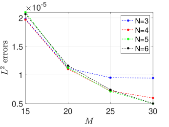
Table 1 shows the spatial -error by increasing and fixing . Tables 2 and 3 show the temporal -errors by taking and increasing under Cases (i) and (ii) in above, respectively. From Tables 1-3, the second order convergence rates can be observed, which agrees with the results in Theorem 4.1. In addition, The left panel in Figure 1 plots the -error by fixing and increasing , which implies that the error estimate is unconditionally stable since the solution does not blowup for any temporal and spatial ratios.
error order 40 4.2893e-05 – 4.6836 80 8.9895e-06 2.2544 4.8091 160 1.9913e-06 2.1745 4.7541 320 4.6221e-07 2.1071 4.7043
error order 120 3.6800e-06 – 4.2785 240 8.3695e-07 2.1365 4.6672 480 1.9795e-07 2.0800 4.1304 960 4.8114e-08 2.0406 4.2979

error order 120 3.6533e-06 – 21.6746 240 8.3479e-07 2.1297 24.1472 480 1.9783e-07 2.0772 285.448 960 4.7942e-08 2.0449 792.551
Example 5.2. We now consider a 3D nonlinear parabolic equation
In the simulations, we take the final time and the computational domain . Again, as a benchmark solution, we take an exact solution in the form of , and the source term can be calculated accordingly.
Table 4 shows the spatial -error by increasing and fixing . Tables 5 and 6 show the temporal -errors by taking and increasing under Cases (i) and (ii) in above, respectively. From Tables 4-6, the second order convergence rates can be observed, which again agrees with the results in Theorem 4.1. The right panel in Figure 1 plots the -error by fixing and increasing , which again implies that the error estimate is unconditionally stable since the solution does not blowup for any temporal and spatial ratios.
error order 6 1.3595e-04 – 4.5317 12 3.3786e-05 2.0086 4.3782 24 8.4315e-06 2.0025 4.3911 48 2.1069e-06 2.0007 4.6375
error order 4 3.0607e-04 – 2.3893 8 7.5914e-05 2.0114 2.2410 16 1.8918e-05 2.0046 2.9583 32 4.7170e-06 2.0038 3.9028
error order 4 3.0721e-04 – 2.4017 8 7.5918e-05 2.0167 13.2425 16 1.8929e-05 2.0039 32.1533 32 4.7200e-06 2.0037 25.1107
6 Conclusions
We have presented the unconditionally optimal error estimate of a linearized variable-time-step BDF2 scheme for nonlinear parabolic equations in conjunction with a Galerkin finite element approximation in space. The rigorous error estimate of in the -norm has been established under mild assumptions on the ratio of adjacent time steps A1 and the maximum time-step size A2. The analysis is based on the recently developed DOC and DCC kernels and the time-space error splitting approach. The techniques of DOC and DCC kernels facilitate the proof of the second order convergence of BDF2 with a new ratio of adjacent time steps, i.e., . The error splitting approach divides the error estimate of numerical solution into the estimates of and , which circumvents the ratio restriction of time-space sizes, i.e., this is the so-called unconditionally optimal error estimate.
In addition, our error estimate is robust. The robustness here means the error estimate does not require any extra restriction on time steps except the conditions A1 and A2. Meanwhile, we used the first-order BDF1 to calculate the first level solution , and found that this first-order scheme did not bring the loss of global accuracy of second order. Although a great progress has been made for the second order convergence of variable time-step BDF2 scheme solving nonlinear problems, but most of them use the implicit approximation to the nonlinear terms. As far as we know, it is a pioneer work to present the optimal error estimate for the variable time-step BDF2 scheme with a linearized approximation to nonlinear terms only under the ratio condition and a mild assumption on maximum time step A2. Numerical examples were provided to verify our theoretical analysis.
Acknowledgements
The research is supported by the National Natural Science Foundation of China (Nos. 11771035 and 12171376), 2020- JCJQ-ZD-029, NSAF U1930402. The numerical calculations in this paper have been done on the supercomputing system in the Supercomputing Center of Wuhan University. JZ would like to thank professor Tao Tang and professor Zhimin Zhang for their valuable discussions on this topic.
7 Appendix
7.1 The proof of Lemma 3.2
Proof. It follows from the Taylor expansion that
where is used. The proof is completed.
7.2 The proof Lemma 3.3
References
- [1] J. Becker. A second order backward difference method with variable steps for a parabolic problem. BIT, 34(4):644–662, 1998.
- [2] W. Chen, X. Wang, Y. Yan, and Z. Zhang. A second order BDF numerical scheme with variable steps for the cahn-hilliard equation. SIAM J. Numer. Anal., 57(1):495–525, 2019.
- [3] E. Emmrich. Stability and error of the variable two-step BDF for semilinear parabolic problems. J. Appl. Math. Comput., 19:33–55, 2005.
- [4] R. Fisher. The wave of advance of advantageous genes. Annals of Eugencies, 7:355–369, 1937.
- [5] R. Grigorieff. Stability of multistep-methods on variable grids. Numer. Math., 42:359–377, 1983.
- [6] R. Grigorieff. Time discretization of semigroups by the variable two-step BDF method. numerical treatment of differential equations, 121:204–216, 1991.
- [7] R. Grigorieff. On the variable grid two-step BDF method for parabolic equation. TU, Fachbereich 3, 1995.
- [8] M. Leroux. Variable stepsize multistep methods for parabolic problems. SIAM J. Numer. Anal., 19:725–741, 1982.
- [9] B. Li and W. Sun. A new approch to errror analysis of linearized semi-implicit galerkin fems for nonlinear parabolic equations. Int. J. Numer. Anal. Model., 24(1):86–103, 2012.
- [10] D. Li, H. Liao, J. Wang, W. Sun, and J. Zhang. Analysis of l1-galerkin fems for time- fractional nonlinear parabolic problems. Commun. Comput. Phys., 24(1):86–103, 2018.
- [11] D. Li, J. Wang, and J. Zhang. Unconditionally convergent l1-galerkin fems for nonlinear time-fractional schrödinger equations. SIAM J. Sci. Comput., 39(1):A3067–A3088, 2017.
- [12] D. Li, C. Wu, and Z. Zhang. Linearized galerkin fems for nonlinear time fractional parabolic problems with non-smoooth solutions in time direction. J. Sci. Comput., 80:403–419, 2019.
- [13] H. Liao, B. Ji, and L. Zhang. An adaptive BDF2 implicit time-stepping method for the phase field crystal model. IMA J. Numer. Anal., page draa075, 2020.
- [14] H. Liao, D. Li, and J. Zhang. Sharp error estimate of the nonuniform l1 formula for reaction- subdiffusion equations. SIAM J. Numer. Anal., 56-2:1112–1133, 2018.
- [15] H. Liao, X. Song, T. Tang, and T. Zhou. Analysis of the second-order BDF scheme with variable steps for the molecular beam epitaxial model without slope selection. Sci. China Math., 64:887–902, 2021.
- [16] H. Liao, T. Tang, and T. Zhou. On energy stable, maximum-principle preserving, second-order BDF scheme with variable steps for the allen-cahn equation. SIAM J. Numer. Anal., 58(4):2294–2314, 2020.
- [17] H. Liao and Z. Zhang. Analysis of adaptive BDF2 scheme for diffusion equations. Math. Comp., 90:1207–1226, 2021.
- [18] C. Palencia and B. García-Archilla. Stability of multistep methods for sectorial operators in banach spaces. Appl. Numer. Math., 12:503–520, 1993.
- [19] V. Thomée. Galerkin finite element methods for parabolic problems, second edition. Springer-Verlag, 2006.
- [20] W. Wang, Y. Chen, and H. Fang. On the variable two-step imex BDF method for parabolic integro-differential equations with nonsmooth initial data arising in finance. SIAM J. Numer. Anal., 57(3):1289–1317, 2019.
- [21] Y. Zeldovich and D. Frank-Kamenetskii. A theory of thermal propagation of flame, dynamics of curved fronts. Academic Press, pages 131–140, 1988.
- [22] J. Zhang and C. Zhao. Sharp error estimate of BDF2 scheme with variable time steps for linear reaction-diffusion equations. J. Math., https://doi.org/10.13548/j.sxzz.20211014.001, 41(6):471–488, 2021.
- [23] J. Zhang and C. Zhao. Sharp error estimate of BDF2 scheme with variable time steps for molecular beam expitaxial models without slop selection. https://doi.org/10.13140/RG.2.2.24714.59842, 41(6):471–488, 2021.