remarkRemark \newsiamremarkhypothesisHypothesis \newsiamremarkexampleExample \newsiamthmclaimClaim \headersUQ for Large Linear Inverse ProblemsC. Travelletti, D. Ginsbourger, and N. Linde
Uncertainty Quantification and Experimental Design for Large-Scale Linear Inverse Problems under Gaussian Process Priors ††thanks: \fundingThis work was funded by the Swiss National Science Fundation (SNF) through project no. 178858.
Abstract
We consider the use of Gaussian process (GP) priors for solving inverse problems in a Bayesian framework. As is well known, the computational complexity of GPs scales cubically in the number of datapoints. We here show that in the context of inverse problems involving integral operators, one faces additional difficulties that hinder inversion on large grids. Furthermore, in that context, covariance matrices can become too large to be stored. By leveraging recent results about sequential disintegrations of Gaussian measures, we are able to introduce an implicit representation of posterior covariance matrices that reduces the memory footprint by only storing low rank intermediate matrices, while allowing individual elements to be accessed on-the-fly without needing to build full posterior covariance matrices. Moreover, it allows for fast sequential inclusion of new observations. These features are crucial when considering sequential experimental design tasks. We demonstrate our approach by computing sequential data collection plans for excursion set recovery for a gravimetric inverse problem, where the goal is to provide fine resolution estimates of high density regions inside the Stromboli volcano, Italy. Sequential data collection plans are computed by extending the weighted integrated variance reduction (wIVR) criterion to inverse problems. Our results show that this criterion is able to significantly reduce the uncertainty on the excursion volume, reaching close to minimal levels of residual uncertainty. Overall, our techniques allow the advantages of probabilistic models to be brought to bear on large-scale inverse problems arising in the natural sciences. Particularly, applying the latest developments in Bayesian sequential experimental design on realistic large-scale problems opens new venues of research at a crossroads between mathematical modelling of natural phenomena, statistical data science and active learning.
1 Introduction
Gaussian processes (GP) provide a powerful Bayesian approach to regression
(Rasmussen and Williams,, 2006). While traditional regression considers pointwise evaluations
of an unknown function, GPs can also include data in the
form of linear operators (Solak et al.,, 2003; Särkkä,, 2011; Jidling et al.,, 2017; Mandelbaum,, 1984; Tarieladze and Vakhania,, 2007; Hairer et al.,, 2005; Owhadi and Scovel,, 2015; Klebanov et al.,, 2020). This allows GPs to provide a Bayesian framework to address inverse problems
(Tarantola and Valette,, 1982; Stuart,, 2010; Dashti and Stuart,, 2016). Even though GP priors have been shown to perform well on smaller-scale inverse problems, difficulties arise when one tries to apply them to large inverse problems (be it high dimensional or high resolution) and these get worse when one considers sequential data assimilation settings such as in Chevalier et al., 2014a . The main goal of this work is to overcome these difficulties and to provide solutions for scaling GP priors to large-scale Bayesian inverse problems.
Specifically, we focus on a triple intersection of i) linear operator data, ii) large number of prediction points and iii) sequential data acquisition. There exists related works that focus on some of these items individually. For example, methods for extending Gaussian processes to large datasets (Hensman et al.,, 2013; Wang et al.,, 2019) or to a large number of prediction points (Wilson et al.,, 2020) gained a lot of attention over the last years. Also, much work has been devoted to extending GP regression to include linear constraints (Jidling et al.,, 2017) or integral observations (Hendriks et al.,, 2018; Jidling et al.,, 2019). On the sequential side, methods have been developed relying on infinite-dimensional state-space representations (Särkkä et al.,, 2013) and have also been extended to variational GPs (Hamelijnck et al.,, 2021). There are also works that focus on the three aspects at the same time (Solin et al.,, 2015). We note that all these approaches rely on approximations, while our method does not.
The topic of large-scale sequential assimilation of linear
operator data has also been of central interest in the Kalman filter community.
To the best of our knowledge, techniques employed in this framework usually
rely on a low rank representation of the
covariance matrix, obtained either via factorization
(Kitanidis,, 2015) or from an ensemble estimate (Mandel,, 2006).
Our goal in this work is to elaborate similar methods for Gaussian processes
without relying on a particular factorization of the covariance matrix. As stated above, we
focus on the case where:
i) the number of prediction points is large,
ii) the data has to be assimilated sequentially, and
iii) it comes in the form of integral operators observations.
Integral operators are harder to handle than pointwise observations since, when discretized on a grid (which is the usual inversion approach), they turn into a matrix with entries that are not predominantly null, in our
case non-zero for most grid points. For the
rest of this work, we will only consider settings that enjoy these three properties.
This situation is typical
of Bayesian large-scale inverse problems because those are often solved on a discrete
grid, forcing one to consider a large number of prediction points when inverting
at high resolution; besides, the linear operators found in
inverse problems are often of integral form (e.g. gravity,
magnetics).
{example*}
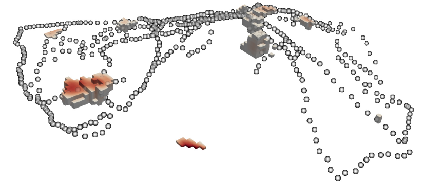
For the rest of this work, we will use as red thread a real-world inverse problem that enjoys the above properties. This problem is that of reconstructing the underground mass density inside the Stromboli volcano, Italy, from observations of the vertical component of the gravity field at different locations of the surface of the volcano (with respect to a reference station), see Fig. 1.


We will use a real dataset of gravimetric observations that was collected during a field campaign in 2012 (courtesy of Linde et al., (2014)). In Linde et al., (2014) the inversion domain is discretized at resolution, which, as we explain in Section 3 results in larger-than-memory covariance matrices, calling for the methods developed in this work.
Our main contribution to overcome the above difficulties is the introduction of
an implicit representation of the posterior covariance matrix that only
requires storage of low rank intermediate matrices and allows
individual elements to be accessed on-the-fly, without ever storing the full
matrix. Our method relies on an extension of the kriging update formulae
(Chevalier et al., 2014c, ; Emery,, 2009; Gao et al.,, 1996; Barnes and Watson,, 1992)
to linear operator observations.
As a minor contribution, we also provide a technique for computing posterior means on fine
discretizations using a chunking technique and explain
how to perform posterior simulations in the considered setting. The developed implicit representation allows for fast updates of posterior covariances under linear
operator observations on very large grids. This is particularly useful when
computing sequential data acquisition plans for inverse problems, which
we demonstrate by computing sequential experimental designs for excursion set learning in
gravimetric inversion. We find that our method provides significant
computational time savings over brute-force conditioning and scales to problem
sizes that are too large to handle using state-of-the-art techniques.
Although the contribution of this work is mostly methodological, the techniques developed here
can be formulated in a rigorous abstract framework by using the language of Gaussian
measures an disintegrations. Though less well-known than GPs,
Gaussian measures provide an equivalent approach (Rajput and Cambanis,, 1972)
that offers several advantages. First, it is more natural for discretization-independent formulations; second, it provides a clear description (in terms of dual spaces) of the observation operators for which a posterior can be defined and third in integrates well with excursion set estimation.
Readers interessted in the technical details are refered to the results in (Travelletti and Ginsbourger,, 2022) upon which we build our implicit representation framework.
To demonstrate our method, we apply it to the Stromboli inverse problem described above. In this context, we show how it allows computing the posterior at high resolution, how hyperparameters of the prior can be trained and how we can sample from the posterior on a large grid. Finally, we illustrate how our method may be applied to a state-of-the-art sequential experimental design task for excursion set recovery. Sequential design criterion for excursion sets have gained a lot of attention recently (Azzimonti et al.,, 2019), but, to the best of our knowledge, this is the first time that sequential experimental design for set estimation is considered in the setting of Bayesian inverse problems.
2 Computing the Posterior under Operator Observations: Bottlenecks and Solutions
In this section, we focus on the challenges that arise when using Gaussian process priors to
solve Bayesian inverse problems with linear operators observations and propose solutions
to overcome these. Here an inverse problem is the task of recovering some unknown function from observation of a bounded linear operator applied to . To solve the problem within a Bayesian framework, one puts a Gaussian process prior on and uses the conditional law of the process, conditional on the data, to approximate the unknown .
Even if one can formulate the problem in an infinite dimensional setting (Travelletti and Ginsbourger,, 2022) and discretization should take place as late as possible (Stuart,, 2010), when solving inverse problems in practice there is always some form of discretization involved, be it through quadrature methods (Hansen,, 2010) or through basis expansion (Wagner et al.,, 2021). It turns out that, regardless of the type of discretization used, one quickly encounters computational bottlenecks arising from memory limitations when trying to scale inversion to real-world problems.
We here focus on inverse problems discretized on a grid, but stress that the computational difficulties described next also plague spectral approaches.
Let be a given set of discretization points, we consider observation operators that (after discretization) may be written as linear combinations of Dirac delta functionals
| (1) |
with arbitrary coefficients . Using (Travelletti and Ginsbourger,, 2022, Corollary 5) we can compute the conditional law of a GP on conditionally on the data , where is some observational noise. The conditional mean and covariance are then given by:
| (2) | ||||
| (3) |
Notation: When working with discrete operators as in Eq. 1 it is more convenient to use matrices. Hence we will use to denote the matrix with elements . Relation Eq. 1 will then be written compactly as . Similarly, given a Gaussian process on and another set of points , we will
use to denote the matrix obtained by evaluating
the covariance function at all couples of points .
In a similar fashion, let denote the vector obtained by concatenating the values of the field at the different points.
From now on, boldface letters will be used to denote concatenated
quantities (usually datasets). The identity matrix will be denoted by , the dimension
being infered from the context.
Even if Eqs. 2 and 3 only involve basic matrix operations, their computational cost depends heavily on the number of prediction points and on the number of discretization points , making their application to real-world inverse problems a non-trivial task. Indeed, when both and are big, there are two main difficulties that hamper the computation of the conditional distribution:
-
•
the matrix may never be built in memory due to its size, and
-
•
the posterior covariance may be too large to store.
The first of these difficulties can be solved by performing the product in chunks, as described in Section 2.3. The second one only becomes of particular interest in sequential data assimilation settings as considered in Section 2.1. In Section 2.2 we will introduce an (almost) matrix-free implicit representation of the posterior covariance matrix enabling us to overcome both these memory bottlenecks.
2.1 Sequential Data Assimilation in Bayesian Inverse Problems and Update Formulae
We now consider a sequential data assimilation problem where data is made available in discrete stages. At each stage, a set of observations described by a (discretized) operator is made and one observes a realization of
| (4) |
where is some set of points in . Then, the posterior mean and covariance after each stage of observation may be obtained by performing a low rank update of their counterparts at the previous stage. Indeed, (Travelletti and Ginsbourger,, 2022, Corollary 6) provides an extension of Chevalier et al., 2014c ; Emery, (2009); Gao et al., (1996); Barnes and Watson, (1992) to linear operator observations, and gives:
Theorem 2.1.
Let and let and denote the conditional mean and covariance function conditional on the data with defined as in Eq. 4, where and and are used to denote the prior mean and covariance. Then:
with , defined as:
At each stage , these formulae require computation of the matrix , which involves a
matrix inversion, where
is the dimension of the operator describing the
current dataset to be included. This allows computational savings by reusing already computed quantities, avoiding inverting the full dataset at each stage, which would require a
matrix inversion, where .
In order for these update equations to bring computational savings, one has to be able to store the past covariances (Chevalier et al.,, 2015). This makes their application to large-scale sequential Bayesian inverse problems difficult, since the covariance matrix on the full discretization may become too large for storage above a certain number of discretization points. The next section presents our main contributions to overcome this limitation. They rely on an implicit representation of the posterior covariance that allows the computational savings offered by the kriging update formulae to be brought to bear on large scale inverse problems.
2.2 Implicit Representation of Posterior Covariances for Sequential Data Assimilation in Large-Scale Bayesian Inverse Problems
We consider the same sequential data assimilation setup as in the previous section,
and for the sake of simplicity we assume that
and use the lighter notation and
. The setting we are interested in here is the one where is so large that
the covariance matrix gets bigger than the
available computer memory.
Our key insight is that instead of building the full posterior covariance at each stage , one can just maintain a routine that computes the product of the current posterior covariance with any other low rank matrix. More precisely, at each stage , we provide a routine (Algorithm 1), that allows to compute the product of the current covariance matrix with any thin matrix :
where thin is to be understood as small enough so that the result of
the multiplication can fit in memory.
This representation of the posterior covariance was inspired by the covariance operator of Gaussian measures. Indeed, if we denote by the covariance operator of the Gaussian measure associated to the posterior distribution of the GP at stage , then
Hence, the procedure may be thought of as computing the action of the covariance operator of the Gaussian measure associated to the posterior on the Dirac delta functionals at the discretization points.
This motivates us to think in terms of an updatable covariance object,
where the inclusion of new observations (the updating) amounts to redefining
a right-multiplication routine.
It turns out that by grouping terms appropriately in Theorem 2.1 such a routine may be defined by only storing low rank
matrices at each data acquisition stage.
Lemma 2.2.
For any and any matrix :
with intermediate matrices and defined as:
Hence, in order to compute products with the posterior covariance at stage , one only has to store matrices , each of size and matrices of size , where is the number of observations made at stage (i.e. the number of lines in ). In turn, each of these objects is defined by multiplications with the covariance matrix at previous stages, so that one may recursively update the multiplication procedure . Algorithms 1, LABEL:, 2, and 3 may be used for multiplication with the current covariance matrix, update of the representation and update of the posterior mean.
2.3 Prior Covariance Multiplication Routine and Chunking
To use Algorithm 1, one should be able to compute products with the prior covariance matrix . This may be achieved by chunking the set of grid points into subsets , where each contains a subset of the points. Without loss of generality, we assume all subsets to have the same size . We may then write the product as
Each of the subproducts may then be performed separately and the results
gathered together at the end. The individual products then involve matrices of
size and . One can then choose
the number of chunks so that these matrices can fit in memory.
Each block may be built on-demand provided
is defined through a given covariance function.
This ability of the prior covariance to be built quickly on-demand
is key to our
method. The fact that the prior covariance matrix does not need to be stored
allows us to handle larger-than-memory posterior covariances by
expressing products with it as a multiplication with the prior and a sum of
multiplications with lower rank matrices.
Remark 2.3 (Choice of Chunk Size).
Thanks to chunking, the product may be computed in parallel, allowing for significant performance improvements in the presence of multiple computing devices (CPUs, GPUs, …). In that case, the chunk size should be chosen as large as possible to limit data transfers, but small enough so that the subproducts may fit on the devices.
2.4 Computational Cost and Comparison to Non-Sequential Inversion
For the sake of comparison, assume that all n datasets have the same size and let denote the total data size. The cost of computing products with the current posterior covariance matrix at some intermediate stage is given by:
Lemma 2.4 (Multiplication Cost).
Let be an matrix. Then, the cost of computing at some stage using Algorithms 1 and 2 is .
Using this recursively, we can then compute the cost of creating the implicit representation of the posterior covariance matrix at stage :
Lemma 2.5 (Implicit Representation Cost).
To leading order in and , the cost of defining is . This is also the cost of computing .
This can then be compared with a non-sequential approach where all datasets would be concatenated into a single dataset of dimension . More precisely, define the matrix and the -dimensional vector as the concatenations of all the measurements and data vectors into a single operator, respectively vector. Then computing the posterior mean using Eq. 2 with those new observation operators and data vector the cost is, to leading order in and :
In this light, we can now sum up the two main advantages of the proposed sequential approach:
-
•
the cubic cost arising from the inversion of the data covariances is decreased to in the sequential approach
-
•
if a new set of observations has to be included, then the direct approach will require the computation of the product , which can become prohibitively expensive when the number of prediction points is large, whereas the sequential approach will only require a marginal computation of .
Aside from the computational cost, our implicit representation also provides significant memory savings compared to an explicit approach where the full posterior covariance matrix would be stored. The storage requirement for the implicit-representation as a function of the number of discretization points is shown in Figure 2.

2.5 Toy Example: 2D Fourier Transform
To illustrate the various methods presented in Section 2.2, we here apply them to a toy two-dimensional example:
we consider a GP discretized on a large square grid and try to learn it through various types of linear operator data.
More precisely, we will here allow two types of observations: pointwise field values and Fourier coefficient data.
Indeed, the field values at the nodes are entirely determined by its discrete Fourier transform (DFT):
| (5) |
Note that the above may be viewed as the discretized version of some operator and thus fits our framework for sequential conditioning. One may then answer questions such as how much uncertainty is left after the first 10 Fourier coefficient have been observed? Or which Fourier coefficient provide the most information about the GP?


For example, Fig. 3 compares the posterior mean after observation of various Fourier coefficients, compared to observing pointwise values along a space-filling sequence. The GP model is a constant mean Matérn random field on a square domain . The domain is discretized onto a grid. Note that, by nature, each Fourier coefficient involves the field values at all points of the discretization grid and thus direct computation of the posterior mean requires the full covariance matrix (which would translate to roughly 100 GB of storage). This makes this situation suitable to demonstrate the techniques presented in this section.
In this example, the Fourier coefficients are ordered by growing norm. One observes that Fourier coefficients provide very different information than pointwise observations and decrease uncertainty in a more spatially uniform way, as shown in Fig. 4.


The extent to which Fourier coefficients provide more or less information than pointwise observations (depending on ordering) depends on the correlation length of the field’s covariance function. Indeed, for long correlation lengths, the low frequency Fourier coefficients contain most of the information about the field’s global behaviour, whereas for small correlation length, high frequency coefficients are needed to learn the small-scale structure.
3 Application: Scaling Gaussian Processes to Large-Scale Inverse Problems
In this section, we demonstrate how the implicit representation of the posterior covariance introduced in Section 2.2 allows scaling Gaussian processes to situations that are too large to handle using more traditional techniques. Such situations are frequently encountered in large-scale inverse problems and we will thus focus our exposition on such a problem arising in geophysics. In this setting, we demonstrate how our implicit representation allows to train prior hyperparameters in Section 3.1, in Section 3.2 we demonstrate posterior sampling on large grids and finally in Section 3.3 address a state-of-the-art sequential experimental design problem for excursion set recovery.
Example Gravimetric Inverse Problem: We focus on the problem of reconstructing the mass density distribution in some given underground domain from observations of the vertical component of the gravitational field at points on the surface of the domain. Such gravimetric data are extensively used on volcanoes (Montesinos et al.,, 2006; Represas et al.,, 2012; Linde et al.,, 2017) and can be acquired non-destrucively at comparatively low costs by 1-2 persons in rough terrain using gravimeters, without the need for road infrastructure or other installations (such as boreholes) that are often lacking on volcanoes. Gravimeters are sensitive to spatial variations in density, which makes them useful to understand geology, localize ancient volcano conduits and present magma chambers, and to identify regions of loose light-weight material that are prone to landslides that could in the case of volcanic islands generate tsunamis.
As an example dataset we use gravimetric data gathered on the surface of the Strombli volcano during a field campaign in 2012 (Linde et al.,, 2014). In Section 3.3 we will also consider the problem of recovering high (or low) density regions inside the volcano. Fig. 5 displays the main components of the problem.


The observation operator describing gravity measurements is an integral one (see Appendix A), which, after discretization, fits the Bayesian inversion framework of Section 2. Indeed, this kind of problems is usually discretized on a finite grid of points , hence the available data is of the form
| (6) |
where the matrix represents the discretized version of the observation operator for the gravity field at and we assume i.i.d Gaussian noise . The posterior may then be computed using Eqs. 2 and 3. Note that the three-dimensional nature of the problem quickly makes it intractable for traditional inversion methods as the resolution of the inversion grid is refined. For example, when discretizing the Stromboli inversion domain as Linde et al., (2014) into cubic cells of side length, one is left with roughly cells, which translates to posterior covariance matrices of size (using 32 bits floating point numbers). This characteristic of gravimetric inverse problems make them well-suited to demonstrate the implicit representation framework which we introduced in Section 2.2. In Section 3.3 we will show how our technique allows state-of-the-art adaptive design techniques to be applied to large real-world problems.
3.1 Hyperparameter Optimization
When using Gaussian process priors to solve inverse problems, one has to select the hyperparameters of the prior. There exists different approaches for optimizing hyperparameters. We here only consider maximum likelihood estimation (MLE).
We restrict ourselves to GP priors that have a constant prior mean and a covariance kernel that depends on a prior variance parameter and other correlation parameters :
| (7) |
where is a correlation function, such that . The maximum likelihood estimator for the hyperparameters may then be obtained by minimizing the negative marginal log likelihood (nmll) of the data, which in the discretized setting of Section 2 may be writen as (Rasmussen and Williams,, 2006):
| (8) | ||||
| (9) |
Since only the quadratic term depends on , we can adapt concentration identities (Park and Baek,, 2001) to write the optimal as a function of the other hyperparameters:
| (10) |
where denotes the -dimensional column vector containing only ’s. Here we always assume to be invertible. The remaining task is then to minimize the concentrated nmll:
Note that the main computational challenge in the minimization of Eq. 8 comes from the presence of the matrix . In the following, we will only consider the case of kernels that depend on a single length scale parameter: , though the procedure described below can in principle be adapted for multidimensional .
In practice, for kernels of the form Eq. 7 the prior variance may be factored out of the covariance matrix (for known noise variance), so that only the prior length scale appears in this large matrix. One then optimizes these parameters separately, using chunking (Section 2.3) to compute matrix products. Since only appears in an matrix which does not need to be chunked (the data size being moderate in real applications), one can use automatic differentiation libraries such as Paszke et al., (2019) to optimize it by gradient descent. On the other hand, there is no way to factor out out of the large matrix , so we resort to a brute force approach by specifying a finite search space for it. To summarize, we proceed here in the following way:
-
(i)
(brute force search) Discretize the search space for the length scale by only allowing , where is a discrete set (usually equally spaced values on a reasonable search interval);
-
(ii)
(gradient descent) For each possible value of , minimize the (concentrated) over the remaining free parameter by gradient descent.
We ran the above approach on the Stromboli dataset with standard stationary kernels (Matérn , Matérn , exponential). In agreement with Linde et al., (2014), the observational noise standard deviation is . The optimization results for different values of the length scale parameter are shown in Fig. 6. The best estimates of the parameter values for each kernel are shown in Table 1. The table also shows the practical range which is defined as the distance at which the covariance falls to of its original value.


We asses the robustness of each kernel by predicting a set of left out observations using the other remaining observations. Fig. 7 displays RMSE and negative log predictive density for different proportion of train/test splits.
| Hyperparameters | Metrics | |||||||
|---|---|---|---|---|---|---|---|---|
| Kernel | Train RMSE | |||||||
| Exponential | 1925.0 | 5766.8 | 535.4 | 308.9 | -804.4 | 0.060 | ||
| Matérn 3/2 | 651.6 | 1952.0 | 2139.1 | 284.65 | -1283.5 | 0.071 | ||
| Matérn 5/2 | 441.1 | 1321..3 | 2120.9 | 349.5 | -1247.6 | 0.073 | ||


Note the the above procedure is more of a quality assurance than a rigorous statistical evaluation of the model, since all datapoints were already used in the fitting of the hyperparameters. Due to known pathologies of the exponential kernel (MLE for length scale parameter going to infinity), we choose to use the Matérn 3/2 model for the experiments of Section 3.2 and Section 3.3. The maximum likelihood estimator of the prior hyperparameters for this model are , and .
3.2 Posterior Sampling
Our implicit representation also allows for efficient sampling from the posterior by
using the residual kriging algorithm (Chilès and Delfiner,, 2012; de Fouquet,, 1994), which we here adapt to linear operator observations. Note that in order to sample a Gaussian process at sampling points, one needs to generate correlated Gaussian random variables, which involves covariance matrices of size , leading to the same computational bottlenecks as described in Section 2. On the other hand, the residual kriging algorithm generates realizations from the
posterior by updating realizations of the prior, as we explain next.
As before, suppose we have a GP defined on some compact Euclidean domain and assume has continuous sample paths almost surely. Furthermore, say we have observations described by linear operators . Then the conditional expectation of conditional on the -algebra is an orthogonal projection (in the -sense (Williams,, 1991)) of onto . This orthogonality can be used to decompose the conditional law of conditional on into a conditional mean plus a residual. Indeed, if we let be another GP with the same distribution as and let , then we have the following equality in distribution:
| (11) |
Compared to direct sampling of the posterior, the above approach involves two main operations: sampling from the prior and conditioning under operator data. When the covariance kernel is stationary and belongs to one of the usual families (Gaussian, Matérn), methods exist to sample from the prior on large grids (Mantoglou and Wilson,, 1982); whereas the conditioning part may be performed using our implicit representation.
Remark 3.1.
Note that in a sequential setting as in Section 2.1, the residual kriging algorithm may be used to maintain an ensemble of realizations from the posterior distribution by updating a fixed set of prior realizations at every step in the spirit of Chevalier et al., (2015).
3.3 Sequential Experimental Design for Excursion Set Recovery
As a last example of application where our implicit update method provides substantial savings, we consider a sequential data collection task involving an inverse problem. Though sequential design criterion for inverse problems have already been considered in the litterature (Attia et al.,, 2018), most of them only focus on selecting observations to improve the reconstruction of the unknown parameter field, or some linear functional thereof.
We here consider a different setting. In light of recent progress in excursion set estimation (Azzimonti et al.,, 2016; Chevalier et al.,, 2013), we instead focus on the task of recovering an excursion set of the unknown parameter field , that is, we want to learn the unknown set , where is some threshold. In the present context of Stromboli, high density areas are related to dykes (previous feeding conduits of the volcano), while low density values are related to deposits formed by paroxysmal explosive phreato-magmatic events (Linde et al.,, 2014). To the best of our knowledge such sequential experimental design problems for excursion set learning in inverse problems have not been considered elsewhere in the litterature.
Remark 3.2.
For the sake of simplicity, we focus only on excursion sets above some threshold, but all the techniques presented here may be readily generalized to generalized excursion sets of the form where is any finite union of intervals on the extended real line.


We here consider a sequential setting, where observations are made one at a time and at each stage we have to select which obsevation to make next in order to optimally reduce the uncertainty on our estimate of .
Building upon Picheny et al., (2010); Bect et al., 2012a ; Azzimonti et al., (2019); Chevalier et al., 2014a ,
there exists several families of criteria to select the next observations. Here, we
restrict ourselves to a variant of the weighted IMSE criterion (Picheny et al.,, 2010). The
investigation of other state-of-the-art criteria is left for future work. We note in passing that most Bayesian sequential design criteria
involve posterior covariances and hence tend to become
intractable for large-scale problems. Moreover in a sequential setting, fast updates of the posterior covariance are crucial. Those
characteristics make the problem considered here particularly suited for the implicit update framework intoduced in Section 2.2.
The weighted IMSE criterion selects next observations by maximizing the variance reduction they will provide at each location, weighted by the probability for that location to belong to the excursion set . Assuming that data collection stages have already been performed and using the notation of Section 2.1, the variant that we are considering here selects the next observation location by maximizing the weighted integrated variance reduction (wIVR):
| (12) |
where is some potential observation location, denotes the conditional covariance after including a gravimetric observation made at (this quantity is independent of the observed data) and is the forward operator corresponding to this observation. Also, here denotes the coverage function at stage (we refer the reader to Appendix B for more details on Bayesian set estimation). After discretization, applying Theorem 2.1 turns this criterion into:
| (13) |
where we have assumed that all measurements are affected by distributed noise.
Note that for large-scale problems, the wIVR criterion in the form
given in Eq. 13 becomes intractable for traditional methods
because of the presence of the full
posterior covariance matrix in the parenthesis.
The implicit representation presented in Section 2.2 can be used
to overcome this difficulty. Indeed, the criterion can be evaluated
using the posterior covariance multiplication routine Lemma 2.2
(where the small dimension is now equal to the number of candidate observations considered
at a time, here but batch acquisition scenarios could also be tackled).
New observations can be seamlessly integrated along the way by updating the representation
using Algorithm 2.
Experiments and Results:
We now study how the wIVR criterion can help to reduce the uncertainty on excursion sets within the Stromboli volcano. We here focus on recovering the volume of the excursion set instead of its precise location.
To the best of our knowledge, in the existing literature such sequential design criteria for excursion set recovery have only been applied to small-scale inverse problems and have not been scaled to larger, more realistic problems where the dimensions at play prevent direct access to the posterior covariance matrix.
In the following experiments, we use the Stromboli volcano inverse problem and work with a discretization into cubic cells of side length. We use a Matérn GP prior with hyperparameters trained on real data (Table 1) to generate semi-realistic ground truths for the experiments. We then simulate numerically the data collection process by computing the response that results from the considered ground truth and adding random observational noise. When computing sequential designs for excursion set estimation, the threshold that defines the excursion set can have a large impact on the accuracy of the estimate. Indeed, different thresholds will produce excursion sets of different sizes, which may be easier or harder to estimate depending on the set estimator used. For the present problem, Fig. 9 shows the distribution of the excursion volume under the considered prior for different excursion thresholds.

It turns out that the estimator used in our experiments (Vorob’ev expectation) behaves differently depending on the size of the excursion set to estimate. Indeed, the Vorob’ev expectation tends to produce a smoothed version of the true excursion set, which in our situation results in a higher fraction of false positives for larger sets. Thus, we consider two scenarios: a large scenario where the generated excursion sets have a mean size of of the total inversion volume and a small scenario where the excursion sets have a mean size of of the total inversion volume. One should note that those percentages are in broad accordance with the usual size of excursion sets that are of interest in geology. The chosen thresholds are for the large excursions and for the small ones.


The experiments are run on five different ground truths, which are samples from a Matérn GP prior (see previous paragraphs). The samples were chosen such that their excursion set for the large scenario have volumes that correspond to the , , , and quantiles of the prior excursion volume distribution for the corresponding threshold. Fig. 10 shows the prior excursion volume distribution together with the volumes of the five different samples used for the experiments. Fig. 11 shows a profile of the excursion set (small scenario) for one of the five samples used in the experiments. The data collection location from the 2012 field campaign (Linde et al.,, 2014) are denoted by black dots. The island boundary is denoted by blue dots. Note that, for the sake of realism, in the experiments we only allow data collection at locations that are situated on the island (data acquired on a boat would have larger errors); meaning that parts of the excursion set that are outside of the island will be harder to recover.


Experiments are run by starting at a fixed starting point on the volcano surface, and then sequentially choosing the next observation locations on the volcano surface according to the wIVR criterion. Datapoints are collected one at a time. We here only consider myopic optimization, that is, at each stage, we select the next observation site according to:
where ties are broken arbitrarily. Here is a set of candidates among which to pick the next observation location. In our experiments, we fix to consist of all surface points within a ball of radius meters around the last observation location. Results are summarized in Figs. 12 and 13, which shows the evolution of the fraction of true positives and false positives as a function of the number of observations gathered.


We see that in the large scenario (Fig. 12) the wIVR criterion is able to correctly detect 70 to 80% of the excursion set (in volume) for each ground truth after 450 observations. For the small scenario (Fig. 13) the amount of true positives reached after 450 observations is similar, though two ground truths are harder to detect.
Note that in Figs. 12 and 13 the fraction of false negatives is expressed as a percentage of the volume of the complementary of the true excursion set . We see that the average percentage of false positives after observations tends to lie between and , with smaller excursion sets yielding fewer false positives. While the Vorob’ev expectation is not designed to minimize the amount of false positives, there exists conservative set estimators (Azzimonti et al.,, 2019) that specialize on this task. We identify the extension of such estimators to inverse problems as a promising venue for new research.


In both figures we also plot the fraction of true positives and false positives that result from the data collection plan that was used in Linde et al., (2014). Here only the situation at the end of the data collection process is shown. We see that for some of the ground truths the wIVR criterion is able to outperform static designs by around 10%. Note that there are ground truths where it performs similarly to a static design. We believe this is due to the fact that for certain ground truths most of the information about the excursion set can be gathered by spreading the observations across the volcano, which is the case for the static design that also considers where it is practical and safe to measure.


Limiting Distribution: The dashed horizontal lines in Figs. 12 and 13 show the detection percentage that can be achieved using the limiting distribution. We define the limiting distribution as the posterior distribution one were to obtain
if one had gathered data at all allowed locations (everywhere on the volcano surface). This distribution may be approximated by gathering data at all points of a given (fine grained) discretization of the surface. In general, this is hard to compute since it requires ingestion of a very large amount of data, but thanks to our implicit representation (Section 2.2) we can get access to this object, thereby, allowing new forms of uncertainty quantification.
In a sense, the limiting distribution represents the best we can hope for when covering the volcano with this type of measurements (gravimetric). It gives a measure of the residual uncertainty inherent to the type of observations used
(gravimetric). Indeed, it is known that a given density field is not
identifiable from gravimetric data alone (see Blakely, (1995) for example).
Even if gravity data will never allow for a perfect reconstruction of the excursion
set, we can use the limiting distribution to compare the performance of
different sequential design criteria and strategies. It also provides a mean of quantifying the remaining uncertainty under the chosen class of models.
A sensible performance metric
is then the number of observations that a given criterion needs to approach the
minimal level of residual uncertainty which is given by the limiting
distributions.
As a last remark, we stress that the above results and the corresponding reconstruction qualities are tied to an estimator, in our case the Vorob’ev expectation. If one were to use another estimator for the excursion set, those results could change significantly.
Posterior Volume Distribution: Thanks to our extension of the residual kriging algorithm to inverse problems (see Section 3.2), we are able to sample from the posterior at the end of the data collection process. This opens new venues for uncertainty quantification in inverse problems. For example, we can use sampling to estimate the posterior distribution of the excursion volume and estimate the residual uncertainty on the size of the excursion set.


Fig. 15 shows the empirical posterior distribution of the excursion volume for each of the ground truths considered in the preceding experiments. When compared to the prior distribution, Fig. 10, one sees that the wIVR criterion is capable of significantly reducing the uncertainty on the excursion volume. This shows that though the location of the excursion set can only be recovered with limited accuracy, as shown in Figs. 12 and 13, the excursion volume can be estimated quite well. This is surprising given that the criterion used (wIVR) is a very crude one and was not designed for that task. On the other hand, there exist more refined criterion, like the so-called SUR strategies (sequential uncertainty reduction) (Chevalier et al., 2014b, ; Bect et al.,, 2019), among which some were specifically engineered to reduce the uncertainty on the excursion volume (Bect et al., 2012b, ). Even though those criterion are more computationally challenging than the wIVR one, expecially in the considered framework, we identify their application to large Bayesian inverse problem as a promising avenue for future research.
4 Conclusion and Perspectives
Leveraging new results about sequential disintegrations of Gaussian measures (Travelletti and Ginsbourger,, 2022), we have introduced an implicit almost matrix free representation of the posterior covariance of a GP and have demonstrated fast update of the posterior covariance on large grids under general linear functional observations. Our method allows streamline updating and fast extraction of posterior covariance information even when the matrices are larger than the available computing memory. Using our novel implicit representation, we have shown how targeted design criteria for excursion set recovery may be extended to inverse problems discretized on large grids. We also demonstrated UQ on such problems using posterior sampling via residual kriging. Our results suggest that using the considered design criteria allows reaching close-to-minimal levels of residual uncertainty using a moderate number of observations and also exhibit significant reduction of uncertainty on the excursion volume. The GP priors used in this work are meant as a proof of concept and future work should address the pitfalls of such priors, such as lack of positiveness of the realisations and lack of expressivity. Other promising research avenues include extension to multivariate excursions Fossum et al., (2021) and inclusion of more sophisticated estimators such as conservative estimates Azzimonti et al., (2019). On the dynamic programming side, extending the myopic optimization of the criterion to finite horizon optimization in order to provide optimized data collection trajectories is an obvious next step which could have significant impact on the geophysics community. Also, including location dependent observation costs such as accessibility in the design criterion could help provide more realistic observation plans.
Acknowledgements
This work was funded by the Swiss National Science Foundation (SNF) through project no. 178858.
References
- Attia et al., (2018) Attia, A., Alexanderian, A., and Saibaba, A. (2018). Goal-oriented optimal design of experiments for large-scale Bayesian linear inverse problems. Inverse Problems, 34.
- Azzimonti et al., (2016) Azzimonti, D., Bect, J., Chevalier, C., and Ginsbourger, D. (2016). Quantifying uncertainties on excursion sets under a Gaussian random field prior. SIAM/ASA Journal on Uncertainty Quantification, 4(1):850–874.
- Azzimonti et al., (2019) Azzimonti, D., Ginsbourger, D., Chevalier, C., Bect, J., and Richet, Y. (2019). Adaptive design of experiments for conservative estimation of excursion sets. Technometrics, 0(0):1–14.
- Banerjee and Das Gupta, (1977) Banerjee, B. and Das Gupta, S. (1977). Gravitational attraction of a rectangular parallelepiped. Geophysics, 42(5):1053–1055.
- Barnes and Watson, (1992) Barnes, R. J. and Watson, A. (1992). Efficient updating of kriging estimates and variances. Mathematical Geology, 24(1):129–133.
- Bect et al., (2019) Bect, J., Bachoc, F., and Ginsbourger, D. (2019). A supermartingale approach to gaussian process based sequential design of experiments. Bernoulli, 25(4A):2883–2919.
- (7) Bect, J., Ginsbourger, D., Li, L., Picheny, V., and Vazquez, E. (2012a). Sequential design of computer experiments for the estimation of a probability of failure. Statistics and Computing, 22(3):773–793.
- (8) Bect, J., Ginsbourger, D., Li, L., Picheny, V., and Vazquez, E. (2012b). Sequential design of computer experiments for the estimation of a probability of failure. Statistics and Computing, 22(3):773–793.
- Blakely, (1995) Blakely, R. J. (1995). Potential Theory in Gravity and Magnetic Applications. Cambridge University Press.
- (10) Chevalier, C., Bect, J., Ginsbourger, D., Vazquez, E., Picheny, V., and Richet, Y. (2014a). Fast parallel kriging-based stepwise uncertainty reduction with application to the identification of an excursion set. Technometrics, 56(4):455–465.
- (11) Chevalier, C., Bect, J., Ginsbourger, D., Vazquez, E., Picheny, V., and Richet, Y. (2014b). Fast parallel kriging-based stepwise uncertainty reduction with application to the identification of an excursion set. Technometrics, 56(4):455–465.
- Chevalier et al., (2015) Chevalier, C., David, G., and Emery, X. (2015). Fast update of conditional simulation ensembles. Mathematical Geosciences, 47:771–789.
- Chevalier et al., (2013) Chevalier, C., Ginsbourger, D., Bect, J., and Molchanov, I. (2013). Estimating and quantifying uncertainties on level sets using the Vorob’ev expectation and deviation with Gaussian process models. In mODa 10–Advances in Model-Oriented Design and Analysis, pages 35–43. Springer.
- (14) Chevalier, C., Ginsbourger, D., and Emery, X. (2014c). Corrected kriging update formulae for batch-sequential data assimilation. In Pardo-Igúzquiza, E., Guardiola-Albert, C., Heredia, J., Moreno-Merino, L., Durán, J., and Vargas-Guzmán, J., editors, Mathematics of Planet Earth. Lecture Notes in Earth System Sciences. Springer, Berlin, Heidelberg.
- Chilès and Delfiner, (2012) Chilès, J.-P. and Delfiner, P. (2012). Geostatistics: Modeling Spatial Uncertainty. Wiley, 2 edition.
- Dashti and Stuart, (2016) Dashti, M. and Stuart, A. M. (2016). The Bayesian approach to inverse problems. Handbook of Uncertainty Quantification, pages 1–118.
- de Fouquet, (1994) de Fouquet, C. (1994). Reminders on the conditioning kriging. In Armstrong, M. and Dowd, P. A., editors, Geostatistical Simulations, pages 131–145, Dordrecht. Springer Netherlands.
- Emery, (2009) Emery, X. (2009). The kriging update equations and their application to the selection of neighboring data. Computational Geosciences, 13(3):269–280.
- Fossum et al., (2021) Fossum, T. O., Travelletti, C., Eidsvik, J., Ginsbourger, D., and Rajan, K. (2021). Learning excursion sets of vector-valued Gaussian random fields for autonomous ocean sampling. The Annals of Applied Statistics, 15(2):597 – 618.
- Gao et al., (1996) Gao, H., Wang, J., and Zhao, P. (1996). The updated kriging variance and optimal sample design. Mathematical Geology, 28(3):295–313.
- Hairer et al., (2005) Hairer, M., Stuart, A. M., Voss, J., and Wiberg, P. (2005). Analysis of SPDEs arising in path sampling. Part I: The Gaussian case. Communications in Mathematical Sciences, 3(4):587 – 603.
- Hamelijnck et al., (2021) Hamelijnck, O., Wilkinson, W. J., Loppi, N. A., Solin, A., and Damoulas, T. (2021). Spatio-temporal variational gaussian processes. In Beygelzimer, A., Dauphin, Y., Liang, P., and Vaughan, J. W., editors, Advances in Neural Information Processing Systems, volume 34. Curran Associates, Inc.
- Hansen, (2010) Hansen, P. C. (2010). Discrete Inverse Problems. Society for Industrial and Applied Mathematics.
- Hendriks et al., (2018) Hendriks, J. N., Jidling, C., Wills, A., and Schön, T. B. (2018). Evaluating the squared-exponential covariance function in gaussian processes with integral observations.
- Hensman et al., (2013) Hensman, J., Fusi, N., and Lawrence, N. D. (2013). Gaussian processes for big data. In Nicholson, A. E. and Smyth, P., editors, Proceedings of the Twenty-Ninth Conference on Uncertainty in Artificial Intelligence, UAI 2013, Bellevue, WA, USA, August 11-15, 2013. AUAI Press.
- Jidling et al., (2019) Jidling, C., Hendriks, J., Schön, T. B., and Wills, A. (2019). Deep kernel learning for integral measurements.
- Jidling et al., (2017) Jidling, C., Wahlström, N., Wills, A., and Schön, T. B. (2017). Linearly constrained gaussian processes. In Guyon, I., Luxburg, U. V., Bengio, S., Wallach, H., Fergus, R., Vishwanathan, S., and Garnett, R., editors, Advances in Neural Information Processing Systems, volume 30. Curran Associates, Inc.
- Kitanidis, (2015) Kitanidis, P. K. (2015). Compressed state Kalman filter for large systems. Advances in Water Resources, 76:120 – 126.
- Klebanov et al., (2020) Klebanov, I., Sprungk, B., and Sullivan, T. J. (2020). The linear conditional expectation in hilbert space.
- Linde et al., (2014) Linde, N., Baron, L., Ricci, T., Finizola, A., Revil, A., Muccini, F., Cocchi, L., and Carmisciano, C. (2014). 3-D density structure and geological evolution of Stromboli volcano (Aeolian Islands, Italy) inferred from land-based and sea-surface gravity data. Journal of Volcanology and Geothermal Research, 273:58–69.
- Linde et al., (2017) Linde, N., Ricci, t., Baron, L., A., S., and G., B. (2017). The 3-D structure of the Somma-Vesuvius volcanic complex (Italy) inferred from new and historic gravimetric data. Scientific Reports, 7(1):8434.
- Mandel, (2006) Mandel, J. (2006). Efficient implementation of the ensemble Kalman filter. Technical Report 231, University of Colorado at Denver and Health Sciences Center.
- Mandelbaum, (1984) Mandelbaum, A. (1984). Linear estimators and measurable linear transformations on a hilbert space. Zeitschrift für Wahrscheinlichkeitstheorie und Verwandte Gebiete, 65(3):385–397.
- Mantoglou and Wilson, (1982) Mantoglou, A. and Wilson, J. L. (1982). The turning bands method for simulation of random fields using line generation by a spectral method. Water Resources Research, 18(5):1379–1394.
- Molchanov, (2005) Molchanov, I. (2005). Theory of random sets. Springer.
- Montesinos et al., (2006) Montesinos, F. G., Arnoso, J., Benavent, M., and Vieira, R. (2006). The crustal structure of El Hierro (Canary Islands) from 3-D gravity inversion. Journal of Volcanology and Geothermal Research, 150(1-3):283–299.
- Owhadi and Scovel, (2015) Owhadi, H. and Scovel, C. (2015). Conditioning gaussian measure on hilbert space.
- Park and Baek, (2001) Park, J.-S. and Baek, J. (2001). Efficient computation of maximum likelihood estimators in a spatial linear model with power exponential covariogram. Computers & Geosciences, 27(1):1–7.
- Paszke et al., (2019) Paszke, A., Gross, S., Massa, F., Lerer, A., Bradbury, J., Chanan, G., Killeen, T., Lin, Z., Gimelshein, N., Antiga, L., Desmaison, A., Kopf, A., Yang, E., DeVito, Z., Raison, M., Tejani, A., Chilamkurthy, S., Steiner, B., Fang, L., Bai, J., and Chintala, S. (2019). Pytorch: An imperative style, high-performance deep learning library. In Wallach, H., Larochelle, H., Beygelzimer, A., d'Alché-Buc, F., Fox, E., and Garnett, R., editors, Advances in Neural Information Processing Systems 32, pages 8024–8035. Curran Associates, Inc.
- Picheny et al., (2010) Picheny, V., Ginsbourger, D., Roustant, O., Haftka, R., and Kim, N. (2010). Adaptive designs of experiments for accurate approximation of a target region. Journal of Mechanical Design, 132:071008.
- Rajput and Cambanis, (1972) Rajput, B. S. and Cambanis, S. (1972). Gaussian processes and Gaussian measures. Ann. Math. Statist., 43(6):1944–1952.
- Rasmussen and Williams, (2006) Rasmussen, C. E. and Williams, C. K. I. (2006). Gaussian Processes for Machine Learning. The MIT Press.
- Represas et al., (2012) Represas, P., Catalão, J. a., Montesinos, F. G., Madeira, J., Mata, J. a., Antunes, C., and Moreira, M. (2012). Constraints on the structure of Maio Island (Cape Verde) by a three-dimensional gravity model: imaging partially exhumed magma chambers. Geophysical Journal International, 190(2):931–940.
- Robbins, (1944) Robbins, H. E. (1944). On the Measure of a Random Set. The Annals of Mathematical Statistics, 15(1):70 – 74.
- Särkkä, (2011) Särkkä, S. (2011). Linear operators and stochastic partial differential equations in Gaussian process regression. In International Conference on Artificial Neural Networks, pages 151–158. Springer.
- Särkkä et al., (2013) Särkkä, S., Solin, A., and Hartikainen, J. (2013). Spatiotemporal learning via infinite-dimensional bayesian filtering and smoothing: A look at gaussian process regression through kalman filtering. IEEE Signal Process. Mag., 30(4):51–61.
- Solak et al., (2003) Solak, E., Murray-Smith, R., Leithead, W. E., Leith, D. J., and Rasmussen, C. E. (2003). Derivative observations in Gaussian process models of dynamic systems. In Advances in neural information processing systems, pages 1057–1064.
- Solin et al., (2015) Solin, A., Kok, M., Wahlström, N., Schön, T., and Särkkä, S. (2015). Modeling and interpolation of the ambient magnetic field by gaussian processes. IEEE Transactions on Robotics, PP.
- Stuart, (2010) Stuart, A. M. (2010). Inverse problems: A Bayesian perspective. Acta Numerica, 19:451–559.
- Tarantola and Valette, (1982) Tarantola, A. and Valette, B. (1982). Generalized nonlinear inverse problems solved using the least squares criterion. Reviews of Geophysics, 20(2):219–232.
- Tarieladze and Vakhania, (2007) Tarieladze, V. and Vakhania, N. (2007). Disintegration of Gaussian measures and average-case optimal algorithms. Journal of Complexity, 23(4):851 – 866. Festschrift for the 60th Birthday of Henryk Woźniakowski.
- Travelletti and Ginsbourger, (2022) Travelletti, C. and Ginsbourger, D. (2022). Disintegration of gaussian measures for sequential assimilation of linear operator data. arXiv, abs/2207.13581.
- Wagner et al., (2021) Wagner, P.-R., Marelli, S., and Sudret, B. (2021). Bayesian model inversion using stochastic spectral embedding. Journal of Computational Physics, 436:110141.
- Wang et al., (2019) Wang, K., Pleiss, G., Gardner, J., Tyree, S., Weinberger, K. Q., and Wilson, A. G. (2019). Exact Gaussian processes on a million data points. In Wallach, H., Larochelle, H., Beygelzimer, A., d’ Alché-Buc, F., Fox, E., and Garnett, R., editors, Advances in Neural Information Processing Systems 32, pages 14622–14632. Curran Associates, Inc.
- Williams, (1991) Williams, D. (1991). Probability with Martingales. Cambridge University Press.
- Wilson et al., (2020) Wilson, J. T., Borovitskiy, V., Terenin, A., Mostowsky, P., and Deisenroth, M. (2020). Efficiently sampling functions from Gaussian process posteriors. ArXiv, abs/2002.09309.
Appendix A Forward operator for Gravimetric Inversion
Given some subsurface density inside a domain and some location outside the domain, the vertical component of the gravitational field at is given by:
| (14) |
with Green kernel
| (15) |
where denotes the vertical component of .
We discretize the domain into identic cubic cells with centroids and assume the mass density to be constant over each cell, so the field may be approximated by the vector . The vertical component of the gravitational field at is then given by:
Integrals of Green kernels over cuboids may be computed using the Banerjee formula (Banerjee and Das Gupta,, 1977).
Theorem A.1 (Banerjee).
The vertical gravity field at point generated by a prism with corners , of uniform mass density is given by:
Appendix B Bayesian Inversion and Bayesian Set Estimation
Given a generic Bayesian linear inverse problem with unknown function and prior , there exists several approaches to approximate the excursion set using the posterior. For example, a naive estimate for may be obtained using the plug-in estimator:
where denotes the posterior mean function of the GP prior. In this work, we will focus on recently developed more sophisticated approaches to Bayesian excursion set estimation (Azzimonti et al.,, 2016; Chevalier et al.,, 2013) based on the theory of random sets (Molchanov,, 2005). We here briefly recall some theory taken from the aforementioned source.
In the following, let denote a random field on that is distributed according to the posterior distribution. Then, the posterior distribution of the field gives rise to a random closed set (RACS):
| (16) |
One can then consider the probability for any point in the domain to belong to that random set. This is captured by the coverage function:
The coverage function allows us to define a parametric family of set estimates for , the Vorob’ev quantiles:
| (17) |
The family of quantiles gives us a way to estimate by controlling the (pointwise) probability that the members of our estimate lie in . There exists several approaches for choosing . One could for example choose it so as to produce conservative estimates of the excursion set (Azzimonti et al.,, 2019). Another approach is to choose it such that the volume of the resulting quantile is equal to the expected volume of the excursion set. This gives rise to the Vorob’ev expectation.
Definition B.1.
(Vorob’ev Expectation) The Vorob’ev expectation is the quantile with threshold chosen such that
where denotes the volume under the Lebesgue measure on .
Note that the expected excursion volume may be computed using Robbins’s theorem, which states that under suitable conditions:
We refer the reader to Robbins, (1944) and Molchanov, (2005) for more details.
To illustrate the various Bayesian set estimation concepts introduced here, we apply them to a simple one-dimensional inverse problem, where one wants to estimate the excursion set above of a function after 3 pointwise evaluations of the function have been observed. Results are shown in Appendix B


Appendix C Proofs
Proof C.1.
(Lemma 2.2) We proceed by induction. The case follows from Eq. 3. The induction step is directly given by Theorem 2.1.
Proof C.2.
(Lemma 2.4) The product is computed using Algorithm 1. It involves multiplication of with the prior covariance, which costs and multiplication with all the previous intermediate matrices, which contribute and respectively, at each stage.
Proof C.3.
(Lemma 2.5) The cost of computing the -th pushforward is . Summing this cost for all stages then gives . To that cost, one should add the cost of computing , which costs at each stage, yielding a contribution to the total cost, which is dominated by since .
Appendix D Supplementary Experimental Results
We here include more detailed analysis of the results of Section 3.3 that do not fit in the main text.
Figs. 12 and 13 showed that there are differences in detection performance for the different ground truths. These can be better understood by plotting the actual location of the excursion set for each of the ground truths as well as the observation locations chosen by the wIVR criterion, as done in Appendix D. One sees that the (comparatively) poor performance shown by Fig. 13 for Sample 2 in the small scenario may be explained by the fact that, for this ground truth, the excursion set is located mostly outside of the accessible data collection zone (island surface), so that the strategy is never able to collect data directly above the excursion.


