Uncertainty Intervals for Prediction Errors in Time Series Forecasting

We provide a simulation example to illustrate the difference between stochastic and expected test errors in time series forecasting, and compare naive FCV and QFCV methods, where the former is a naive CLT-based uncertainty interval (Eq (12) in Section 4.1) as a baseline and the latter is our proposed uncertainty interval that will be elaborated in Algorithm 1 in Section 3. At each time step $t\in\{1,\ldots,1000\}$, we observe feature vector $x_{t}\in{\mathbb{R}}^{p}$ where $p=20$, with IID standard normal entries, and outcomes $y_{t}=x_{t}^{\sf{T}}\beta+\varepsilon_{t}$ following a linear model. Here $\beta=(1,1,1,1,0,\ldots)^{\sf{T}}\in\mathbb{R}^{p}$, and noise $\{\varepsilon_{t}\}_{t=1}$ is an AR(1) process with parameter $\phi=0.5$. The forecaster is a Lasso regression trained on the last $40$ time indices ($961$ to $1000$). Our target is the prediction error over the unseen future $20$ data points ($1001$ to $1020$).

We calculate the coverage of naive FCV and QFCV intervals over $500$ simulation instances. Figure 1 shows these intervals for the first 50 instances. Numerical results demonstrate $90\%$ nominal coverage by QFCV for the stochastic test error, which we theoretically justify in Section 3. In contrast, FCV severely undercovers the stochastic test error at only $12.8\%$ coverage, and slightly undercovers the expected test error at $78.0\%coverage$. In Section 4, we explain the issues with naive FCV and investigate certain correction approaches. Overall, this example illustrates the difference between stochastic and expected test errors in time series, and shows that QFCV provides valid coverage while naive FCV does not.

This paper provides a systematic investigation of inference for prediction errors in time series forecasting. We identify two inferential targets, the stochastic test error and the expected test error, and discuss different methods for providing uncertainty intervals. Our contribution is three-fold.

• •

  We propose quantile-based forward cross-validation (QFCV) methods to provide prediction intervals for stochastic test error (Section 3). We prove that QFCV methods have asymptotically valid coverage under the assumption of ergodicity. Through numerical simulations, we show that QFCV methods give well-calibrated coverages. In particular, when choosing an appropriate auxiliary function, QFCV provides shorter intervals than the naive empirical quantile method, especially for smooth time series.

• •

  We examine forward cross-validation (FCV) methods, which are CLT-based procedures adapted from cross-validation in the IID setting (Section 4). These methods seem like a natural choice for practitioners. We identify issues with the naive FCV method that underlie its failure to cover the stochastic and expected test errors. We also investigate two modifications to naive FCV that partially address these problems. However, these modifications do not perfectly restore valid coverage without strong assumptions.

• •

  For non-stationary time series, we provide rolling intervals by combining the QFCV method with a variant of the adaptive conformal inference, which we name the AQFCV method (Section 5). AQFCV method produces rolling intervals with asymptotically valid time-average coverage under arbitrary non-stationarity. We articulate the difference between time-average coverage and the frequentist’s notion of instance-average coverage. Finally, we demonstrate AQFCV’s performance on both simulated and real-world time series data.

In stationary time series, a straightforward approach for providing a prediction interval involves estimating the quantile of the stochastic prediction error distribution using the observed dataset. We introduce a more refined method named Quantile-based Forward Cross-Validation (QFCV). In a nutshell, QFCV estimates the quantile function of the stochastic prediction error, $\textup{Err}_{\rm sto}$, based on certain user-specified features. These features are expected to have high predictive power to $\textup{Err}_{\rm sto}$, an example being the validation error.

To introduce QFCV, we organize the time indices into multiple possibly overlapping time windows, which we denote as $\{D_{i},V_{i},D_{i\star},T_{i}\}_{i\in[K]}$ and $\{D,V,D_{\star},T\}$, as depicted in Figure 3. The time windows $\{D_{i},D_{i\star},D,D_{\star}\}$ share the same size, denoted as ${n_{\sf tr}}$; $\{V_{i},V\}$ share the same size, denoted as ${n_{\sf val}}$; $\{T_{i},T\}$ share the same size, denoted as ${n_{\sf te}}$. In addition, for each $i\in[K]$, each time window in $\{D_{i+1},V_{i+1},D_{(i+1)\star},T_{i+1}\}$ shifts from $\{D_{i},V_{i},D_{i\star},T_{i}\}$ by $\Delta$ indices, where $\Delta(K-1)+{n_{\sf tr}}+{n_{\sf val}}+{n_{\sf te}}\leq{n}$. Spelling out the elements of each time window, we have

	$\displaystyle D_{i}=$	$\displaystyle\leavevmode\nobreak\ \{(i-1)\Delta+1,\ldots,{(i-1)\Delta+{n_{\sf tr}}}\},\leavevmode\nobreak\ \leavevmode\nobreak\ \leavevmode\nobreak\ \leavevmode\nobreak\ \leavevmode\nobreak\ \leavevmode\nobreak\ \leavevmode\nobreak\ \leavevmode\nobreak\ \leavevmode\nobreak\ \leavevmode\nobreak\ \leavevmode\nobreak\ \leavevmode\nobreak\ \leavevmode\nobreak\ \leavevmode\nobreak\ \leavevmode\nobreak\ \leavevmode\nobreak\ \leavevmode\nobreak\ \leavevmode\nobreak\ \leavevmode\nobreak\ \leavevmode\nobreak\ \leavevmode\nobreak\ D=\{{n}-{n_{\sf tr}}-{n_{\sf val}}+1,\ldots,{n}-{n_{\sf val}}\},$		(5)
	$\displaystyle V_{i}=$	$\displaystyle\leavevmode\nobreak\ \{(i-1)\Delta+{n_{\sf tr}}+1,\ldots,(i-1)\Delta+{n_{\sf tr}}+{n_{\sf val}}\},\leavevmode\nobreak\ \leavevmode\nobreak\ \leavevmode\nobreak\ \leavevmode\nobreak\ \leavevmode\nobreak\ \leavevmode\nobreak\ \leavevmode\nobreak\ \leavevmode\nobreak\ \leavevmode\nobreak\ \leavevmode\nobreak\ \leavevmode\nobreak\ \leavevmode\nobreak\ \leavevmode\nobreak\ \leavevmode\nobreak\ \leavevmode\nobreak\ \leavevmode\nobreak\ \leavevmode\nobreak\ \leavevmode\nobreak\ \leavevmode\nobreak\ \leavevmode\nobreak\ \leavevmode\nobreak\ V=\{{n}-{n_{\sf val}}+1,\ldots,{n}\},$
	$\displaystyle D_{i\star}=$	$\displaystyle\leavevmode\nobreak\ \{(i-1)\Delta+{n_{\sf val}}+1,\ldots,{(i-1)\Delta+{n_{\sf tr}}+{n_{\sf val}}}\},\leavevmode\nobreak\ \leavevmode\nobreak\ \leavevmode\nobreak\ \leavevmode\nobreak\ \leavevmode\nobreak\ \leavevmode\nobreak\ \leavevmode\nobreak\ \leavevmode\nobreak\ \leavevmode\nobreak\ \leavevmode\nobreak\ \leavevmode\nobreak\ \leavevmode\nobreak\ \leavevmode\nobreak\ \leavevmode\nobreak\ \leavevmode\nobreak\ \leavevmode\nobreak\ \leavevmode\nobreak\ \leavevmode\nobreak\ \leavevmode\nobreak\ \leavevmode\nobreak\ D_{\star}=\{{n}-{n_{\sf tr}}+1,\ldots,{n}\},$
	$\displaystyle T_{i}=$	$\displaystyle\leavevmode\nobreak\ \{(i-1)\Delta+{n_{\sf tr}}+{n_{\sf val}},\ldots,(i-1)\Delta+{n_{\sf tr}}+{n_{\sf val}}+{n_{\sf te}}-1\},\leavevmode\nobreak\ \leavevmode\nobreak\ \leavevmode\nobreak\ \leavevmode\nobreak\ \leavevmode\nobreak\ \leavevmode\nobreak\ \leavevmode\nobreak\ T=\{{n}+1,\ldots,{n}+{n_{\sf te}}\}.$

Furthermore, given a user-specified auxiliary function that generates a set of covariates for predicting the stochastic prediction error, denoted as ${\mathcal{A}}:{\mathcal{Z}}^{{n_{\sf tr}}}\times{\mathcal{Z}}^{{n_{\sf val}}}\to{\mathbb{R}}^{m}$, we define tuples $\{(\textup{Err}_{i}^{{\rm val}},\textup{Err}_{i}^{{\rm test}})\}_{i\in[K]}$ and $(\textup{Err}_{\star}^{\rm val},\textup{Err}_{\star}^{{\rm test}})$ by the equations below:

	$\displaystyle\textup{Err}_{i}^{{\rm val}}=$	$\displaystyle\leavevmode\nobreak\ {\mathcal{A}}(z_{D_{i}},z_{V_{i}})\in{\mathbb{R}}^{m},\leavevmode\nobreak\ \leavevmode\nobreak\ \leavevmode\nobreak\ \leavevmode\nobreak\ \leavevmode\nobreak\ \leavevmode\nobreak\ \leavevmode\nobreak\ \leavevmode\nobreak\ \leavevmode\nobreak\$	$\displaystyle\textup{Err}_{i}^{{\rm test}}=$	$\displaystyle\leavevmode\nobreak\ \textstyle\frac{1}{|T_{i}|}\sum_{t\in T_{i}}\ell(\hat{f}(x_{t};z_{D_{i\star}}),y_{t})\in{\mathbb{R}},$		(6)
	$\displaystyle\textup{Err}_{\star}^{{\rm val}}=$	$\displaystyle\leavevmode\nobreak\ {\mathcal{A}}(z_{D},z_{V})\in{\mathbb{R}}^{m},\leavevmode\nobreak\ \leavevmode\nobreak\ \leavevmode\nobreak\ \leavevmode\nobreak\ \leavevmode\nobreak\ \leavevmode\nobreak\ \leavevmode\nobreak\ \leavevmode\nobreak\ \leavevmode\nobreak\$	$\displaystyle\textup{Err}_{\star}^{{\rm test}}=$	$\displaystyle\leavevmode\nobreak\ \textstyle\frac{1}{|T|}\sum_{t\in T}\ell(\hat{f}(x_{t};z_{D_{\star}}),y_{t})\in{\mathbb{R}}.$

Here, $z_{D}$ is a condensed notation for $\{z_{t}\}_{t\in D}$. It is important to note that $\{(\textup{Err}_{i}^{{\rm val}},\textup{Err}_{i}^{{\rm test}})\}_{i\in[K]}$ and $\textup{Err}_{\star}^{\rm val}$ can be computed from the observed dataset $\{z_{t}\}_{t\in[{n_{\sf tr}}]}$, but $\textup{Err}_{\star}^{{\rm test}}$ depends on future unobserved data points. Indeed, $\textup{Err}_{\star}^{{\rm test}}$ is the same as the stochastic prediction error $\textup{Err}_{\rm sto}$, as defined in Eq. (1). Assuming the time series is stationary, it is evident that $\{(\textup{Err}_{i}^{{\rm val}},\textup{Err}_{i}^{{\rm test}})\}_{i\in[K]}$ and $(\textup{Err}_{\star}^{\rm val},\textup{Err}_{\star}^{{\rm test}})$ are identically distributed, though they are not independent due to time correlation.

The QFCV method, given these definitions, can be summarized in the three steps below. First, calculate $\{(\textup{Err}_{i}^{{\rm val}},\textup{Err}_{i}^{{\rm test}})\}$ and $\textup{Err}_{\star}^{\rm val}$ given by Eq. (6). Then, predict quantiles of $\{\textup{Err}_{i}^{{\rm test}}\}$ based on feature vectors $\{\textup{Err}_{i}^{{\rm val}}\}$ by minimizing the empirical quantile loss to obtain quantile functions $\hat{f}^{\alpha/2}$ and $\hat{f}^{1-\alpha/2}$. Finally, the QFCV prediction interval is given by ${\rm PI}^{\alpha}_{\rm QFCV}=[\hat{f}^{\alpha/2}(\textup{Err}^{{\rm val}}_{\star}),\hat{f}^{1-\alpha/2}(\textup{Err}^{{\rm val}}_{\star})]$. Detailed steps are provided in Algorithm 1.

We provide theoretical guarantees on the coverage of QFCV prediction intervals, under the assumption of a stationary time series. We present methods for relaxing the stationarity assumption in Section 5.

Given this assumption, ${(\textup{Err}_{t}^{{\rm val}},\textup{Err}_{t}^{{\rm test}})}_{t\geq 1}$ is likewise stationary ergodic and shares the same distribution as $(\textup{Err}_{\star}^{{\rm val}},\textup{Err}_{\star}^{{\rm test}})$. Let $\mathcal{L}$ denote this common distribution. For simplicity, we will assume $\mathcal{L}$ has a density with respect to the Lebesgue measure. While this is a strong assumption, it could be relaxed by more sophisticated analysis.

Moreover, we denote ${\mathcal{F}}_{\beta}$ as the class of $\beta$-quantiles of the conditional distribution of $\textup{Err}_{\star}^{{\rm test}}$ given $\textup{Err}_{\star}^{{\rm val}}$. This class can be expressed as minimizers of the pinball loss,

$${\mathcal{F}}_{\beta}=\Big{\{}g^{*}\in\arg\min_{g:{\mathbb{R}}^{m}\to{\mathbb{R}}}{\mathbb{E}}_{{\mathcal{L}}}\big{[}{\sf pinball}_{\beta}\big{(}\textup{Err}^{{\rm test}}-g(\textup{Err}^{{\rm val}})\big{)}\big{]}\Big{\}}.$$

We assume the function class ${\mathcal{F}}$ used in the QFCV algorithm (Algorithm 1) can realize the $\alpha/2$ and $1-\alpha/2$ quantile classes, ${\mathcal{F}}_{\alpha/2}$ and ${\mathcal{F}}_{1-\alpha/2}$. Furthermore, for simplicity, we assume that ${\mathcal{F}}$ is finite, a strong assumption that could also be relaxed.

We are ready to state the asymptotically valid coverage for the QFCV method, as detailed in Theorem 3.1. The proof of this theorem can be found in Appendix A. A more general statement going beyond the finite function class assumption (Assumption 3) can be found in Appendix A.1.

We remark that the choice of the auxiliary function ${\mathcal{A}}:{\mathcal{Z}}^{{n_{\sf tr}}\times{n_{\sf val}}}\to{\mathbb{R}}^{m}$ does not affect the asymptotic validity of QFCV prediction intervals. However, when the dimension $m$ is large, more samples will often be required for the asymptotic regime to take effect. In practice, we would like to choose $m$ to be moderately small and to be some function such that $\textup{Err}_{\star}^{{\rm val}}$ and $\textup{Err}_{\star}^{{\rm test}}$ have a large mutual information.

We evaluate QFCV methods with different choices of auxiliary functions ${\mathcal{A}}$ through a simulation study. Recall the setting as in Section 2, we generate a time series with ${n}=2000$ historical data, train a model on ${n_{\sf tr}}=40$ training set, and aim to construct prediction intervals for the test error over the next ${n_{\sf te}}\in\{5,20\}$ unseen points (see Figure 2 for a diagram of this dataset division). The simulated time series $\{z_{t}\}_{t\geq 1}$ is generated as follows: for each time step $t$, $z_{t}=(x_{t},y_{t})\in{\mathbb{R}}^{p}\times{\mathbb{R}}$ with $p=20$, where

$\displaystyle y_{t}=x_{t}^{\sf{T}}\beta+\varepsilon_{t},\leavevmode\nobreak\ \leavevmode\nobreak\ \leavevmode\nobreak\ \leavevmode\nobreak\ \leavevmode\nobreak\ x_{t}\sim_{iid}{\mathcal{N}}(0,I_{p}),\leavevmode\nobreak\ \leavevmode\nobreak\ \leavevmode\nobreak\ \leavevmode\nobreak\ \leavevmode\nobreak\ \{\varepsilon_{t}\}_{t\geq 1}\sim{\rm ARMA}(a,b).$

(9)

We fix the true coefficient vector as $\beta=(1,1,1,1,0,\ldots,0)^{\sf{T}}\in\mathbb{R}^{p}$, where the first four coordinates are $1$, and the rest of the coordinates are $0$. The noise process $\{\varepsilon_{t}\}_{t\geq 1}$ follows a standard autoregressive-moving-average model $\text{ARMA}(a,b)$ with AR coefficients ${\boldsymbol{\phi}}=(\phi_{1},\ldots,\phi_{a})^{\sf{T}}$ and MA coefficients ${\boldsymbol{\theta}}=(\theta_{1},\ldots,\theta_{b})^{\sf{T}}$. That is

$$\textstyle\varepsilon_{t}=\sum_{k=1}^{a}\phi_{k}\cdot\varepsilon_{t-k}+\eta_{t}+\sum_{i=1}^{b}\theta_{i}\cdot\eta_{t-i},\leavevmode\nobreak\ \leavevmode\nobreak\ \leavevmode\nobreak\ \leavevmode\nobreak\ \leavevmode\nobreak\ \leavevmode\nobreak\ \leavevmode\nobreak\ \leavevmode\nobreak\ \leavevmode\nobreak\ \{\eta_{t}\}_{t\geq 1}\sim_{iid}\sim{\mathcal{N}}(0,1).$$

(10)

We consider two ARMA parameter settings:

• (1)

  $\text{ARMA}(1,0)$ with ${\boldsymbol{\phi}}=\phi\in[0,1]$.

• (2)

  $\text{ARMA}(1,20)$ with ${\boldsymbol{\phi}}=\phi\in[0,1]$ and ${\boldsymbol{\theta}}=(0.1,0.2,\ldots 0.9,1,1,0.9,\ldots,0.1)^{\sf{T}}\in\mathbb{R}^{20}$.

Both processes are stationary, but setting (2) exhibits smoother sample paths than setting (1), as visualized in Figure 5 which plots realizations of $\{\varepsilon_{t}\}_{t\geq 1}$ for the first 200 time steps. We posit that setting (2), as a smoother noise process, will yield a higher correlation between validation and test errors $(\textup{Err}_{\star}^{{\rm val}},\textup{Err}_{\star}^{{\rm test}})$.

We consider QFCV methods utilizing the following auxiliary functions. For $m\in\{1,\ldots,{n_{\sf val}}\}$, we split the validation set $V_{i}$ into $m$ continuous and non-overlapping subsets $V_{i1},\ldots,V_{im}\subseteq V_{i}$. We define the auxiliary function ${\mathcal{A}}_{m}$ of dimension $m$ as the vector of validation errors on each subset:

$${\mathcal{A}}_{m}(z_{D_{i}},z_{V_{i}})=\left(\frac{1}{|V_{i1}|}\sum_{t\in V_{i1}}\ell(\hat{f}(x_{t};z_{D_{i}}),y_{t}),\ldots\frac{1}{|V_{im}|}\sum_{t\in V_{im}}\ell(\hat{f}(x_{t};z_{D_{i}}),y_{t})\right)^{\sf{T}}\in\mathbb{R}^{m}.$$

For $m=0$, we use a trivial auxiliary function ${\mathcal{A}}_{0}(z_{D_{i}},z_{V_{i}})\equiv 1$. We denote by $\text{QFCV}(m)$ the QFCV method utilizing auxiliary function ${\mathcal{A}}_{m}$. We provide a few special examples as follows.

• •

  $\text{QFCV}(0)$: ${\mathcal{A}}_{0}(z_{D_{i}},z_{V_{i}})=1$. Here, QFCV essentially calculates the empirical quantile of $\{\textup{Err}_{i}^{{\rm test}}\}$, equivalent to the intercept-only quantile regression.

• •

  $\text{QFCV}(1)$: ${\mathcal{A}}_{1}(z_{D_{i}},z_{V_{i}})=\frac{1}{|V_{i}|}\sum_{t\in V_{i}}\ell(\hat{f}(x_{t};z_{D_{i}}),y_{t})\in\mathbb{R}$. Here, QFCV uses quantile regression with the single feature given by the average validation error.

• •

  $\text{QFCV}({n_{\sf val}})$: ${\mathcal{A}}_{{n_{\sf val}}}(z_{D_{i}},z_{V_{i}})=(\ell(\hat{f}(x_{t};z_{D_{i}}),y_{t}))_{t\in V_{i}}\in\mathbb{R}^{n_{\sf val}}$. Here, QFCV uses quantile regression with ${n_{\sf val}}$ features given by the individual validation errors.

In all cases, we use linear quantile regression of $\{\textup{Err}_{i}^{{\rm test}}\}$ against $\{\textup{Err}_{i}^{{\rm val}}\}$, choosing ${\mathcal{F}}$ as the class of linear functions.

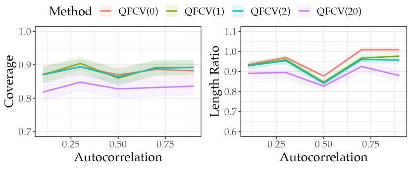
Figure 6 reports the coverage and length of QFCV intervals under different simulation settings. The time series is generated according to model (9), where the noise $\{\varepsilon_{t}\}$ follows either an $\text{ARMA}(1,0)$ process (panels (a) and (c)) or $\text{ARMA}(1,20)$ process (panels (b) and (d)). For both noise processes, we fix the MA coefficients ${\boldsymbol{\theta}}$ and vary the AR coefficient $\phi$ along the x-axis over $[0,1]$ to modulate autocorrelation. The nominal coverage level is $90\%$. To normalize the interval lengths, we divide the QFCV lengths by the true marginal quantiles interval length, defined as the difference between the $95\%$ and $5\%$ quantiles of the true test error distribution. Each curve displays the mean and standard error over $500$ simulation instances.

Figure 6 shows that $\text{QFCV}(m)$ achieves close to $90\%$ coverage at the nominal level when $m$ is less than or equal to $2$. However, for $m=20$ in panels (c) and (d), the coverage deviates further from the nominal level, likely because quantile regression requires more samples to be consistent with a $20$-dimensional feature vector. In terms of interval lengths, all QFCV methods produce similar lengths to the true marginal quantiles on data with non-smooth $\text{ARMA}(1,0)$ noise (panels (a) and (c)). However, for smooth $\text{ARMA}(1,20)$ noise (panels (b) and (d)), $\text{QFCV}(m>0)$ can substantially outperform the true marginal quantiles length, especially when ${n_{\sf val}}=5$ (panel (b)). This occurs because with smooth noise, the validation error $\textup{Err}_{\star}^{{\rm val}}$ becomes more predictive of the actual test error $\textup{Err}_{\star}^{{\rm test}}$.

To explain why $\text{QFCV}(m>0)$ produces smaller average interval lengths than $\text{QFCV}(0)$, Figure 7 presents scatter plots of the length ratios versus true test errors over $500$ simulation instances. The noise process is taken to be $\text{ARMA}(1,20)$ with $\phi=0.9$ and ${n_{\sf val}}=5$. The left panel shows that $\text{QFCV}(0)$ (the empirical quantile method) generates interval lengths close to the true marginal quantiles for all ranges of the true test error. In contrast, $\text{QFCV}(1)$ assigns smaller intervals for small true test errors. The right panel colors points by whether they are mis-covered. We see that while $\text{QFCV}(0)$ tends to mis-cover points with large test errors, the mis-covered points for $\text{QFCV}(>0)$ are more uniformly distributed across the test error range. This indicates that by adapting to the validation error, $\text{QFCV}(>0)$ produces prediction intervals that are overall shorter while maintaining coverage.

Figure 8 shows how the actual coverage of QFCV methods varies with the time series length ${n}$, for an $\text{ARMA}(1,0)$ noise process with $\phi=0.5$ and ${n_{\sf val}}=5$. We find that all QFCV variants achieve close to the nominal $90\%$ coverage when ${n}>1000$. However, using a larger number $m$ of features for quantile regression leads to a larger estimation error, requiring more samples to attain the nominal coverage level. This highlights the need to avoid excessively large $m$ values in practice.

Let us take a moment to reflect on and discuss our main proposal of QFCV prediction intervals for time series forecasting.

In FCV, we split the historical data sequence $z_{1:{n}}$ into $K$ possibly overlapping time windows. Each window is shifted $\Delta$ time steps from the previous one. For the $i$-th window, we further divide it into a training set $D_{i}=\{(i-1)\Delta+1,\ldots,(i-1)\Delta+{n_{\sf tr}}\}$ of size ${n_{\sf tr}}$ and a validation set $V_{i}=\{(i-1)\Delta+{n_{\sf tr}}+1,\ldots,(i-1)\Delta+{n_{\sf tr}}+{n_{\sf val}}\}$ of size ${n_{\sf val}}$. See Figure 9 for a diagram illustration. The FCV point estimate of the prediction error is:

$${\widehat{\rm Err}}_{K}^{\rm FCV}=\frac{1}{K}\sum_{i=1}^{K}\frac{1}{{n_{\sf val}}}\sum_{t\in V_{i}}\ell(\hat{f}(x_{t};z_{D_{i}}),y_{t})=\frac{1}{K}\sum_{i=1}^{K}E_{i},\leavevmode\nobreak\ \leavevmode\nobreak\ \leavevmode\nobreak\ \leavevmode\nobreak\ \text{ where }E_{i}=\frac{1}{{n_{\sf val}}}\sum_{t\in V_{i}}\ell(\hat{f}(x_{t};z_{D_{i}}),y_{t}).$$

(11)

Under the stationary assumption, ${\widehat{\rm Err}}_{K}^{\rm FCV}$ is an unbiased estimator for the expected target error Err, as stated in Lemma 4.1 below.

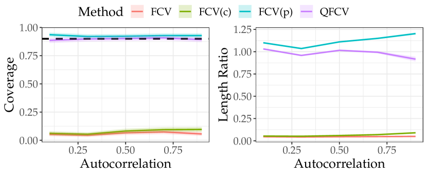
We perform numerical simulations to compare CLT-based FCV intervals (Algorithm 2) with QFCV methods (Algorithm 1). Specifically, we examine naive FCV intervals (FCV), autocorrelation-corrected FCV intervals (FCV(c)), and scaling-corrected FCV intervals (FCV(p)) for the CLT-based methods. For the QFCV method, we use $\text{QFCV}(1)$, where the auxiliary function is the validation error (7). The simulations follow the same setup as in Section 3.3, with time series generated from a linear model (9) with $\text{ARMA}(a,b)$ noise. We investigate the coverage and length ratio of these intervals. The results, presented in Figure 11, illustrate the performance of the different methods.

The results in Figure 11 demonstrate that the naive FCV and FCV(c) methods undercover the stochastic test error $\textup{Err}_{\rm sto}$ across the simulation settings. In contrast, the FCV(p) and QFCV methods achieve valid coverage. However, the QFCV intervals are shorter than those from FCV(p), particularly for time series with smoother noise processes. This aligns with our expectations, as we anticipated FCV(p) would have similar performance to QFCV(0). Since QFCV(1) utilizes features informative to the stochastic test error during quantile regression, it outperforms QFCV(0), and hence should outperform FCV(p).

Table 1 provides further comparison of the four methods across the simulation settings. The first row for each setting shows the mis-coverage percentages of the stochastic test error $\textup{Err}_{\rm sto}$ for both the upper and lower ends. This illustrates that QFCV has more balanced mis-coverage than FCV(p), which is expected since QFCV relies on quantiles, without the need of Gaussian assumptions like FCV(p). The second row for each setting gives the mis-coverage percentages of the expected test error Err. It demonstrates that FCV(c) provides better coverage for Err and serves as a better confidence interval than naive FCV through its autocovariance correction. The fourth row for each setting illustrates the mean squared error of the FCV and QFCV point estimators for estimating the stochastic test error $\textup{Err}_{\rm sto}$. It shows that QFCV point estimator has a smaller MSE than the FCV point estimator.

References

- [AB21] Anastasios N Angelopoulos and Stephen Bates. A gentle introduction to conformal prediction and distribution-free uncertainty quantification. arXiv preprint arXiv:2107.07511, 2021.
- [AC10] Sylvain Arlot and Alain Celisse. A survey of cross-validation procedures for model selection. 2010.
- [All74] David M Allen. The relationship between variable selection and data agumentation and a method for prediction. technometrics, 16(1):125–127, 1974.
- [Avi03] Yossi Aviv. A time-series framework for supply-chain inventory management. Operations Research, 51(2):210–227, 2003.
- [AZ20] Morgane Austern and Wenda Zhou. Asymptotics of cross-validation. arXiv preprint arXiv:2001.11111, 2020.
- [BB11] Christoph Bergmeir and Jose M Benitez. Forecaster performance evaluation with cross-validation and variants. In 2011 11th International Conference on Intelligent Systems Design and Applications, pages 849–854. IEEE, 2011.
- [BB12] Christoph Bergmeir and José M Benítez. On the use of cross-validation for time series predictor evaluation. Information Sciences, 191:192–213, 2012.
- [BBJM20] Pierre Bayle, Alexandre Bayle, Lucas Janson, and Lester Mackey. Cross-validation confidence intervals for test error. Advances in Neural Information Processing Systems, 33:16339–16350, 2020.
- [BCB14] Christoph Bergmeir, Mauro Costantini, and José M Benítez. On the usefulness of cross-validation for directional forecast evaluation. Computational Statistics & Data Analysis, 76:132–143, 2014.
- [BCN94] Prabir Burman, Edmond Chow, and Deborah Nolan. A cross-validatory method for dependent data. Biometrika, 81(2):351–358, 1994.
- [BHK18] Christoph Bergmeir, Rob J Hyndman, and Bonsoo Koo. A note on the validity of cross-validation for evaluating autoregressive time series prediction. Computational Statistics & Data Analysis, 120:70–83, 2018.
- [BHT21] Stephen Bates, Trevor Hastie, and Robert Tibshirani. Cross-validation: what does it estimate and how well does it do it? arXiv preprint arXiv:2104.00673, 2021.
- [Bol86] Tim Bollerslev. Generalized autoregressive conditional heteroskedasticity. Journal of econometrics, 31(3):307–327, 1986.
- [BPvdL20] David Benkeser, Maya Petersen, and Mark J van der Laan. Improved small-sample estimation of nonlinear cross-validated prediction metrics. Journal of the American Statistical Association, 115(532):1917–1932, 2020.
- [BWXB23] Aadyot Bhatnagar, Huan Wang, Caiming Xiong, and Yu Bai. Improved online conformal prediction via strongly adaptive online learning. arXiv preprint arXiv:2302.07869, 2023.
- [Coc97] John H Cochrane. Time series for macroeconomics and finance, 1997.
- [CTM20] Vitor Cerqueira, Luis Torgo, and Igor Mozeti. Evaluating time series forecasting models: An empirical study on performance estimation methods. Machine Learning, 109:1997–2028, 2020.
- [Die98] Thomas G Dietterich. Approximate statistical tests for comparing supervised classification learning algorithms. Neural computation, 10(7):1895–1923, 1998.
- [DZY+17] Chirag Deb, Fan Zhang, Junjing Yang, Siew Eang Lee, and Kwok Wei Shah. A review on time series forecasting techniques for building energy consumption. Renewable and Sustainable Energy Reviews, 74:902–924, 2017.
- [Efr83] Bradley Efron. Estimating the error rate of a prediction rule: improvement on cross-validation. Journal of the American statistical association, 78(382):316–331, 1983.
- [ET97] Bradley Efron and Robert Tibshirani. Improvements on cross-validation: the 632+ bootstrap method. Journal of the American Statistical Association, 92(438):548–560, 1997.
- [FBR22] Shai Feldman, Stephen Bates, and Yaniv Romano. Conformalized online learning: Online calibration without a holdout set. arXiv preprint arXiv:2205.09095, 2022.
- [FH20] Edwin Fong and Chris C Holmes. On the marginal likelihood and cross-validation. Biometrika, 107(2):489–496, 2020.
- [FVD00] Philip Hans Franses and Dick Van Dijk. Non-linear time series models in empirical finance. Cambridge university press, 2000.
- [GC21] Isaac Gibbs and Emmanuel Candès. Adaptive conformal inference under distribution shift. Advances in Neural Information Processing Systems, 34:1660–1672, 2021.
- [GC22] Isaac Gibbs and Emmanuel Candès. Conformal inference for online prediction with arbitrary distribution shifts. arXiv preprint arXiv:2208.08401, 2022.
- [Gei75] Seymour Geisser. The predictive sample reuse method with applications. Journal of the American statistical Association, 70(350):320–328, 1975.
- [Gil05] Kenneth Gilbert. An arima supply chain model. Management Science, 51(2):305–310, 2005.
- [HAB23] Hansika Hewamalage, Klaus Ackermann, and Christoph Bergmeir. Forecast evaluation for data scientists: common pitfalls and best practices. Data Mining and Knowledge Discovery, 37(2):788–832, 2023.
- [Ham20] James Douglas Hamilton. Time series analysis. Princeton university press, 2020.
- [Hay11] Fumio Hayashi. Econometrics. Princeton University Press, 2011.
- [HTFF09] Trevor Hastie, Robert Tibshirani, Jerome H Friedman, and Jerome H Friedman. The elements of statistical learning: data mining, inference, and prediction, volume 2. Springer, 2009.
- [Lei20] Jing Lei. Cross-validation with confidence. Journal of the American Statistical Association, 115(532):1978–1997, 2020.
- [LLC+15] Bo Liu, Jianqiang Li, Cheng Chen, Wei Tan, Qiang Chen, and MengChu Zhou. Efficient motif discovery for large-scale time series in healthcare. IEEE Transactions on Industrial Informatics, 11(3):583–590, 2015.
- [LPvdL15] Erin LeDell, Maya Petersen, and Mark van der Laan. Computationally efficient confidence intervals for cross-validated area under the roc curve estimates. Electronic journal of statistics, 9(1):1583, 2015.
- [LTS22] Zhen Lin, Shubhendu Trivedi, and Jimeng Sun. Conformal prediction intervals with temporal dependence. arXiv preprint arXiv:2205.12940, 2022.
- [MTBH05] Marianthi Markatou, Hong Tian, Shameek Biswas, and George M Hripcsak. Analysis of variance of cross-validation estimators of the generalization error. 2005.
- [MWMC18] Pavol Mulinka, Sarah Wassermann, Gonzalo Marin, and Pedro Casas. Remember the good, forget the bad, do it fast-continuous learning over streaming data. In Continual Learning Workshop at NeurIPS 2018, 2018.
- [NB99] Claude Nadeau and Yoshua Bengio. Inference for the generalization error. Advances in neural information processing systems, 12, 1999.
- [PAA+22] Fotios Petropoulos, Daniele Apiletti, Vassilios Assimakopoulos, Mohamed Zied Babai, Devon K Barrow, Souhaib Ben Taieb, Christoph Bergmeir, Ricardo J Bessa, Jakub Bijak, John E Boylan, et al. Forecasting: theory and practice. International Journal of Forecasting, 2022.
- [Rac00] Jeff Racine. Consistent cross-validatory model-selection for dependent data: hv-block cross-validation. Journal of econometrics, 99(1):39–61, 2000.
- [RT19] Saharon Rosset and Ryan J Tibshirani. From fixed-x to random-x regression: Bias-variance decompositions, covariance penalties, and prediction error estimation. Journal of the American Statistical Association, 2019.
- [SC11] Ingo Steinwart and Andreas Christmann. Estimating conditional quantiles with the help of the pinball loss. 2011.
- [SEJS86] Petre Stoica, Pieter Eykhoff, Peter Janssen, and Torsten Söderström. Model-structure selection by cross-validation. International Journal of Control, 43(6):1841–1878, 1986.
- [Sha93] Jun Shao. Linear model selection by cross-validation. Journal of the American statistical Association, 88(422):486–494, 1993.
- [Sto74] Mervyn Stone. Cross-validatory choice and assessment of statistical predictions. Journal of the royal statistical society: Series B (Methodological), 36(2):111–133, 1974.
- [SV08] Glenn Shafer and Vladimir Vovk. A tutorial on conformal prediction. Journal of Machine Learning Research, 9(3), 2008.
- [SY22] Sophia Sun and Rose Yu. Copula conformal prediction for multi-step time series forecasting. arXiv preprint arXiv:2212.03281, 2022.
- [TT09] Ryan J Tibshirani and Robert Tibshirani. A bias correction for the minimum error rate in cross-validation. 2009.
- [VGS99] Volodya Vovk, Alexander Gammerman, and Craig Saunders. Machine-learning applications of algorithmic randomness. 1999.
- [VS06] Sudhir Varma and Richard Simon. Bias in error estimation when using cross-validation for model selection. BMC bioinformatics, 7(1):1–8, 2006.
- [Wag20] Stefan Wager. Cross-validation, risk estimation, and model selection: Comment on a paper by rosset and tibshirani. Journal of the American Statistical Association, 115(529):157–160, 2020.
- [XX22] Chen Xu and Yao Xie. Sequential predictive conformal inference for time series. arXiv preprint arXiv:2212.03463, 2022.
- [Yan07] Yuhong Yang. Consistency of cross validation for comparing regression procedures. 2007.
- [You20] Waleed A Yousefa. A leisurely look at versions and variants of the cross validation estimator. stat, 1050:9, 2020.
- [You21] Waleed A Yousef. Estimating the standard error of cross-validation-based estimators of classifier performance. Pattern Recognition Letters, 146:115–125, 2021.
- [ZFG+22] Margaux Zaffran, Olivier Féron, Yannig Goude, Julie Josse, and Aymeric Dieuleveut. Adaptive conformal predictions for time series. In International Conference on Machine Learning, pages 25834–25866. PMLR, 2022.
- [Zha93] Ping Zhang. Model selection via multifold cross validation. The annals of statistics, pages 299–313, 1993.
- [Zha95] Ping Zhang. Assessing prediction error in non-parametric regression. Scandinavian journal of statistics, pages 83–94, 1995.
Appendix A Proof of Theorem 3.1
Proof of Theorem 3.1.
Throughout the proof, we take . For general , the proof follows similarly. The proof uses the uniform convergence argument and relies on the following lemma.
Lemma A.1.
Let be random variables that have a joint density with respect to the Lebesgue measure. Define the risk function
Then for any function , we have,
We take and define the empirical risk associated to the -pinball loss as
For and , and for any quantile function , we define