Uncertainty-Aware Robust Learning on Noisy Graphs
Abstract.
Graph neural networks have shown impressive capabilities in solving various graph learning tasks, particularly excelling in node classification. However, their effectiveness can be hindered by the challenges arising from the widespread existence of noisy measurements associated with the topological or nodal information present in real-world graphs. These inaccuracies in observations can corrupt the crucial patterns within the graph data, ultimately resulting in undesirable performance in practical applications. To address these issues, this paper proposes a novel uncertainty-aware graph learning framework motivated by distributionally robust optimization. Specifically, we use a graph neural network-based encoder to embed the node features and find the optimal node embeddings by minimizing the worst-case risk through a minimax formulation. Such an uncertainty-aware learning process leads to improved node representations and a more robust graph predictive model that effectively mitigates the impact of uncertainty arising from data noise. Our experimental result shows that the proposed framework achieves superior predictive performance compared to the state-of-the-art baselines under various noisy settings.
1. Introduction
The field of graph learning has witnessed significant advancements in recent years, fueled by the remarkable performance of graph neural networks (GNNs) (gcn, 1, 2). GNNs leverage message-passing techniques to enable efficient information exchange among nodes in a graph, leading to improved embeddings. Among the various graph-based learning tasks, node classification, especially in a semi-supervised setting, stands out as a prominent and widely applicable problem that has greatly benefited from GNNs. The objective of node classification is to learn high-quality node embeddings and make predictions about their labels using a graph that has only a subset of nodes labeled.
However, similar to other deep neural networks, GNNs are susceptible to the influence of noisy input, including both noisy features and graph structure (li2022recent, 3, 4, 5). This issue becomes even more critical in the low-data setting, where the performance can be greatly impaired by noisy observations when only a limited number of labeled nodes are available (li2022recent, 3, 4, 6). For example, in a social network, new users may inconsistently express their preferences or engage with content that aligns with their actual interests due to limited options available at that time. Such noises would introduce uncertainty and incorrect information about the user’s preferences into the training data. With only a few labeled samples available, the GNN heavily relies on these noisy observations to learn the user’s preferences and generalize them to make less accurate recommendations. Hence, the GNN’s capacity to capture the underlying patterns of different nodes can be significantly compromised when the input graph is noisy.
In this paper, we propose a novel uncertainty-aware graph learning framework based on distributionally robust optimization (DRO) (duchi2021learning, 7, 8, 9, 10). The proposed Distributionally Robust Graph Learning (DRGL) framework significantly improves node embedding quality and enhances model performance, particularly in the presence of noisy data that hinders the direct observation of key graph features. To tackle this challenge, we first allow the underlying node feature patterns to vary within a pre-defined family of distributions and seek the least favorable distribution (LFD) in the worst-case scenario. It is important to note that the uncertainty arising from data noise is represented by an uncertainty set (NEURIPS2018_a08e32d2, 9, 11, 12), characterized by a Wasserstein ball (NEURIPS2018_a08e32d2, 9, 11, 13, 14). Then, by minimizing the risk associated with this worst-case distribution, we can discover the most robust node embeddings that effectively mitigate the impact of uncertainty. To seamlessly integrate this minimax formulation into graph learning, we also leverage differentiable optimization techniques (cvx, 15, 16) and develop a tractable end-to-end learning algorithm. Furthermore, the resulting minimax solution also provides a means to estimate the potential uncertainty associated with predictions, allowing decision-makers to assess the likelihood of different outcomes. This information is particularly valuable in high-stakes scenarios where incorrect decisions can have severe consequences. Lastly, our numerical results demonstrate that the proposed learning strategy significantly enhances the quality of node embeddings and achieves promising predictive performance on semi-supervised node classification when compared to state-of-the-art methods.
Related work. Graph neural networks (GNNs) have emerged as powerful models aiming to learn expressive representations for graph-structure data (gcn, 1, 2, 17, 18). While these approaches proved to be successful (gcn, 1, 2, 19), they are highly sensitive to the quality of the given graphs in terms of either node feature or graph structure (li2022recent, 3, 5). To address the robustness limitations of GNNs in the presence of noises in node features and edges, researchers have explored different methods to purify the noisy graph (li2022recent, 3, 4, 20). For example, graph structure learning designs different graph structure learners to enhance the robustness of GNNs against structure noise (NEURIPS2020_e05c7ba4, 21, 22, 23). Another line of research focuses on improving the robustness of GNNs against inaccurate or missing node features (8970731, 24, 25, 26) through developing noise-resistant aggregation and propagation techniques. However, a major limitation of the existing methods is that they require a task-specific design of structure learning or regularization term to address a certain type of noise, which limits their applicability in more general application settings.
Our approach handles noisy graphs based on the DRO (duchi2021learning, 7, 8), which aims to enhance the robustness of GNNs by minimizing the worst-case risk in the presence of data noise. Only a handful of recent research attempts, such as (zhang2021robust, 11, 27), have embraced similar concepts and investigated the potential applications of DRO in the context of graph-structured data. For instance, Sadeghi et al. (sadeghi2021distributionally, 27) use GNNs to encode the input graph and employ DRO for model training. However, their work is mainly focused on the noisy node features, while we consider a more general scenario involving both noisy features and edges. Furthermore, their method solves for worst-case distribution and updates model parameters separately at each iteration (sadeghi2021distributionally, 27), while our approach offers an end-to-end approach updating parameters with gradient-based learning techniques. Additionally, our approach provides uncertainty quantification under Least Favorable Distributions (LFDs). This capability has meaningful applications in uncertainty-sensitive scenarios (ABDAR2021243, 28, 29), such as molecular classification tasks in graphs (ryu2019bayesian, 30, 31).
2. Uncertainty-aware graph learning
Problem setup. Consider an attributed graph , where represents the set of nodes, and represents the set of edges connecting the nodes. Each node is associated with a -dimensional feature vector . The collection of all node features is denoted as . To describe the graph more generally, we can represent it as , where is the adjacency matrix, which provides information about the connectivity between nodes. If , then ; otherwise, . Each node can be assigned one of the discrete labels . In the context of semi-supervised node classification, we have access to labels for only a subset of nodes, which we denote as , where represents the number of observed nodes. The remaining nodes have no assigned labels and are denoted as . In our setting, the assigned labels are assumed to be correct, but there might be errors or inaccuracies in the observed edges or node features due to noisy measurements. Our objective is to predict the labels for these unobserved nodes in the graph.
Node embedding. We use a graph encoder to embed the node features, including both the nodal information and the corresponding graph structure. We emphasize that our framework is not tied to any specific model and offers flexibility in selecting graph encoders. In this study, we use Graph Convolutional Networks (GCNs) (gcn, 1, 32) and Graph Attention Networks (GATs) (gat, 2) to encode both the node feature and the graph topology. For each node , the graph encoder functions as a nonlinear transformation, denoted as , taking the nodal features and the corresponding graph topology as input and returning their node embeddings, denoted by . Formally,
Here denotes the parameters specific to the model used in our framework.
It is important to note that these node embeddings obtained through minimizing standard loss functions (e.g., sum of squared errors) may not accurately reflect the true feature patterns of the graph due to the presence of noise in the observed data.
Distributionally robust graph learning. To address this issue, we develop a novel graph learning framework that improves the node embeddings, resulting in more robust predictive performance, particularly when confronted with noisy data. Figure 1 summarizes the architecture of the proposed model.
Our approach assumes that node embeddings share the same label adhere to an underlying distribution (), within an uncertainty set encompassing all potential distributions . However, obtaining a direct observation of this distribution is challenging due to inaccuracies in the nodal or topological information, and any changes in node embeddings will influence their corresponding distributions. The key idea of our proposed framework is to find the most robust node embeddings represented by that minimize the worst-case risk over the uncertainty set in the probability simplex . This results in the definition of our distributionally robust minimax problem:
| (1) |
where is the risk function, and we define the risk of a classifier as the summation of error probabilities under each class, i.e., . We note that the optimal solution to the inner maximization problem is known as the least favorable distributions (LFDs) in statistics literature. The risk associated with these distributions is considered the worst-case risk.

As shown in Figure 2, we choose the uncertainty set to be a Wasserstein ball of radius centered at the empirical distribution :
| (2) |
where denotes the set of all probability distributions on . The is defined as , where is some cost function transferring from to , . The empirical distribution is represented by the Dirac point mass, denoted as:
| (3) |
Here, refers to the Dirac delta function, represents the cardinality of a set, and denotes the indicator function.
As the original problem (1) entails an intractable infinite dimensional functional optimization, we follow (NEURIPS2018_a08e32d2, 9, 10) and introduce the proposition below. This proposition reformulates the problem into a computationally tractable convex optimization problem due to our careful selection of the risk function and uncertainty sets.
Proposition 1.
For the uncertainty sets defined in (2), the least favorable distribution of problem (1) can be obtained by solving the following problem:
| (4) | ||||
| subject to | ||||
The decision variable can be viewed as a joint distribution on empirical points with marginal distributions and , represented by a vector . The inequality constraint controls the Wasserstein distance between and .
Remark 1.
The maximization in (4) measures the margin between the maximum likelihood of among all classes and the likelihood of the -th class. Thus, the objective can be equivalently rewritten as the minimization of the total margin. When , the total margin reduces to the total variation distance.

Model estimation. The model estimation can be carried out in an end-to-end fashion. To propagate the error backward through the convex optimization problem described in (4), we adopt the idea of differentiable optimization (DO) (cvx, 15, 16). This approach enables us to differentiate through certain subclasses of convex optimization problems. In other words, the convex solver can be seen as a function that maps the data of the problem to its corresponding solutions, making it amenable to gradient-based learning techniques. Therefore, the learning objective can be jointly written as:
| (5) |
where can be regarded as the output layer of our model, which takes the node embeddings as input and returns their LFDs by solving (4).
We apply the mini-batch stochastic gradient descent as summarized in Algorithm 1.
It is necessary that each mini-batch, which is provided to the convex solver, includes at least one training sample from every class. This requirement is put in place to maintain the integrity of the optimization and its ability to generate valid solutions at all times.
3. Experiments
Experimental setup. In our experiments, we use three widely-used data sets, including Cora (mccallum2000automating, 33), Citeseer (giles1998citeseer, 34), and Pubmed (graphdata, 35). These data sets consist of citation networks among , , and scientific publications, respectively (yang2016revisiting, 36). In these networks, each node represents a text document, and its feature vector corresponds to a bag-of-words representation. We primarily focus on few-shot learning tasks where each data set contains -class and noisy training samples per class.
To assess the robustness of our method, we introduce random noise into these data sets in the following two ways: (1) We add Gaussian noise to the node feature matrix , where is set proportionally to the standard deviation of the bag-of-words representation of all nodes in each graph; (2) We randomly remove a certain percentage of edges in the graph. We repeat each test three times and calculate the average accuracy.
Since our framework is designed to be compatible with various models, we choose to experiment with Graph Convolutional Networks (GCNs) (gcn, 1) and Graph Attention Networks (GATs) (gat, 2) as our graph encoders due to their popularity as competitive baselines. We also evaluate our framework using two commonly used classifiers (output layers), including a shallow (2-layer) neural network with Softmax output and a weighted -NN. To fit the models, we use the Adam optimizer with a learning rate of for all experiments. A more detailed experimental setup can be found in Appendix A.
Main results. We start by examining the impact of random Gaussian noise added to the node features on each method with . Table 1 presents the average classification accuracy, revealing that GCN and GAT models trained with DRGL consistently outperforms the standard models across almost all scenarios using the same classifiers. These findings underscore the effectiveness of DRGL in improving the embedding’s robustness when confronted with noise present in the node features.
Next we assess the performance of DRGL in the missing edge setting with . Table 2 shows that both GCN and GAT equipped with DRGL exhibit substantial improvement, particularly in scenarios where a higher percentage of edges are removed. This showcases the efficacy of DRGL in enhancing the resilience of GNNs when facing challenges associated with missing edges.
We also conduct experiments in the standard few-shot setting using GCN (xu2021dp, 37, 38), where no noise is added to the data. In this setting, each node class is provided with a limited number of labeled samples, along with the original features and edges. The results presented in Table 3 demonstrate that using DRGL in conjunction with GCN yields the highest average test accuracy across all data sets when compared to baseline methods. This indicates that while the DRGL is primarily designed for noisy graphs, it also enhances model performance in standard few-shot scenarios. Additional experimental results can be found in Appendix B.
| Models | Cora (M = 7) | Citeseer (M = 6) | Pubmed (M = 3) | |||||
|---|---|---|---|---|---|---|---|---|
| LP | 47.70 | 47.70 | 21.73 | 21.73 | 28.90 | 28.90 | ||
| GCN+ Softmax | 66.17 | 52.43 | 37.83 | 30.35 | 63.43 | 57.83 | ||
| GAT+ Softmax | 66.48 | 59.03 | 65.90 | 60.43 | 63.73 | 58.70 | ||
| Softmax | 66.20 | 54.40 | 39.80 | 34.90 | 63.20 | 59.70 | ||
| Softmax | 67.83 | 59.40 | 65.60 | 61.27 | 64.57 | 59.77 | ||
-
•
* takes value of one or two standard deviation of the nodal features.
| Models | Cora (M = 7) | Citeseer (M = 6) | Pubmed (M = 3) | |||||
|---|---|---|---|---|---|---|---|---|
| LP | 41.67 | 32.10 | 17.83 | 11.60 | 26.53 | 23.53 | ||
| GCN+ Softmax | 67.30 | 50.83 | 39.25 | 35.70 | 66.07 | 62.07 | ||
| GAT+ Softmax | 67.28 | 57.08 | 64.07 | 60.13 | 64.80 | 61.96 | ||
| Softmax | 66.70 | 52.15 | 40.15 | 41.80 | 66.63 | 64.30 | ||
| Softmax | 69.02 | 58.88 | 65.93 | 61.20 | 65.93 | 60.53 | ||
-
•
* is the edge removal percentage.
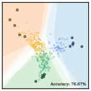
Learned embeddings and their uncertainty. To gain a more intuitive understanding of the learned embedding space produced by DRGL, we conducted an additional ablation study. In this study, we represent the learned node embeddings in a two-dimensional (2D) space and visualize them as a scatter plot. Figure 3 and Figure 4 give real examples using three classes of nodes from Cora data set (mccallum2000automating, 33). In these figures, the training data points are represented by large dots, while the testing data points are represented by small dots. The color of the dots corresponds to their true categories, providing a visual reference. The color depth of the regions suggests the likelihood of a sample being classified into the predicted category.
Figure 3 presents a comparison between the learned node embeddings and those generated by the vanilla GCN in various scenarios. We can observe that the between-class distance demonstrates a slight increase in contrast to the vanilla GCN. Conversely, the intra-class distance shows a minor reduction, as denoted by the denser distribution of dots with matching colors. It is worth mentioning that such differences in distribution can become more prominent in higher dimensional embedding spaces. Although seemingly subtle, this shift in the distribution of embeddings plays a pivotal role in significantly improving the accuracy of the classification outcomes, indicated by the numbers displayed in the lower right corner.
Figure 4 showcases the visual representation of the LFDs generated by DRGL. The shades of grey in the visualization are obtained using kernel density estimation, where darker shades indicate a higher level of uncertainty between the different categories. These LFDs serve as a valuable tool for uncertainty quantification (UQ), enabling us to pinpoint the data points that are susceptible to the greatest impact in worst-case scenarios. Let denote the predicted probabilities of a classifier built on learned LFDs of a graph. The predictive uncertainty can be expressed using entropy (6769090, 39, 40, 41). The result highlights the improved capability of our approach in capturing and quantifying uncertainty compared with the vanilla GCN method.
| Models | Cora (M = 7) | Citeseer (M = 6) | Pubmed (M = 3) | |||||
|---|---|---|---|---|---|---|---|---|
| K = 5 | K = 10 | K = 5 | K = 10 | K = 5 | K = 10 | |||
| LP | 47.70 | 52.80 | 21.73 | 28.33 | 28.90 | 38.63 | ||
| GCN+ -NN | 36.20 | 66.50 | 28.50 | 52.47 | 45.57 | 68.27 | ||
| GCN+ Softmax | 63.47 | 70.67 | 45.37 | 57.83 | 67.10 | 71.27 | ||
| -NN | 44.60 | 68.23 | 34.07 | 53.30 | 51.10 | 68.67 | ||
| Softmax | 66.13 | 72.60 | 49.83 | 59.33 | 67.83 | 72.20 | ||


4. Conclusion
To address the challenges posed by noisy graphs, we proposed a novel GNN-agnostic framework that enhances the robustness of node embeddings and predictive performance. Particularly, our proposed framework improves the model robustness by accounting for the uncertainties raised by the data noise within the graph, which shows substantial improvements over state-of-the-art baselines on different benchmark datasets.
References
- (1) Thomas N Kipf and Max Welling “Semi-Supervised Classification with Graph Convolutional Networks” In arXiv preprint arXiv:1609.02907, 2016
- (2) Petar Veličković et al. “Graph Attention Networks”, 2018 arXiv:1710.10903 [stat.ML]
- (3) Jintang Li et al. “Recent Advances in Reliable Deep Graph Learning: Inherent Noise, Distribution Shift, and Adversarial Attack” In arXiv e-prints, 2022, pp. arXiv–2202
- (4) Yanqiao Zhu et al. “A survey on graph structure learning: Progress and opportunities” In arXiv e-prints, 2021, pp. arXiv–2103
- (5) Dongsheng Luo et al. “Learning to Drop: Robust Graph Neural Network via Topological Denoising” In Proceedings of the 14th ACM International Conference on Web Search and Data Mining, WSDM ’21 Virtual Event, Israel: Association for Computing Machinery, 2021, pp. 779–787 DOI: 10.1145/3437963.3441734
- (6) Kaize Ding et al. “Toward robust graph semi-supervised learning against extreme data scarcity” In arXiv preprint arXiv:2208.12422, 2022
- (7) John C Duchi and Hongseok Namkoong “Learning models with uniform performance via distributionally robust optimization” In The Annals of Statistics 49.3 Institute of Mathematical Statistics, 2021, pp. 1378–1406
- (8) Shai Shalev-Shwartz and Yonatan Wexler “Minimizing the maximal loss: How and why” In International Conference on Machine Learning, 2016, pp. 793–801 PMLR
- (9) Rui Gao, Liyan Xie, Yao Xie and Huan Xu “Robust Hypothesis Testing Using Wasserstein Uncertainty Sets” In Advances in Neural Information Processing Systems 31 Curran Associates, Inc., 2018 URL: https://proceedings.neurips.cc/paper_files/paper/2018/file/a08e32d2f9a8b78894d964ec7fd4172e-Paper.pdf
- (10) Shixiang Zhu et al. “Distributionally robust weighted k-nearest neighbors” In Advances in Neural Information Processing Systems 35, 2022, pp. 29088–29100
- (11) Xiang Zhang et al. “Robust Graph Learning Under Wasserstein Uncertainty”, 2021 arXiv:2105.04210 [cs.LG]
- (12) Rizal Fathony et al. “Distributionally robust graphical models” In Advances in Neural Information Processing Systems 31, 2018
- (13) Matthew Staib and Stefanie Jegelka “Distributionally robust deep learning as a generalization of adversarial training” In NIPS workshop on Machine Learning and Computer Security 3, 2017, pp. 4
- (14) Soroosh Shafieezadeh Abadeh, Peyman M Mohajerin Esfahani and Daniel Kuhn “Distributionally robust logistic regression” In Advances in Neural Information Processing Systems 28, 2015
- (15) A. Agrawal et al. “Differentiable Convex Optimization Layers” In Advances in Neural Information Processing Systems, 2019
- (16) Brandon Amos and J. Kolter “OptNet: Differentiable Optimization as a Layer in Neural Networks” In Proceedings of the 34th International Conference on Machine Learning 70, Proceedings of Machine Learning Research PMLR, 2017, pp. 136–145
- (17) Joan Bruna, Wojciech Zaremba, Arthur Szlam and Yann LeCun “Spectral Networks and Locally Connected Networks on Graphs”, 2014 arXiv:1312.6203 [cs.LG]
- (18) Michaël Defferrard, Xavier Bresson and Pierre Vandergheynst “Convolutional Neural Networks on Graphs with Fast Localized Spectral Filtering” In Advances in Neural Information Processing Systems, 2016 URL: https://arxiv.org/abs/1606.09375
- (19) Petar Velickovic et al. “Deep graph infomax.” In ICLR (Poster) 2.3, 2019, pp. 4
- (20) Kaize Ding, Zhe Xu, Hanghang Tong and Huan Liu “Data augmentation for deep graph learning: A survey” In ACM SIGKDD Explorations Newsletter, 2022
- (21) Yu Chen, Lingfei Wu and Mohammed Zaki “Iterative Deep Graph Learning for Graph Neural Networks: Better and Robust Node Embeddings” In Advances in Neural Information Processing Systems 33 Curran Associates, Inc., 2020, pp. 19314–19326 URL: https://proceedings.neurips.cc/paper_files/paper/2020/file/e05c7ba4e087beea9410929698dc41a6-Paper.pdf
- (22) Wei Jin et al. “Graph Structure Learning for Robust Graph Neural Networks” In Proceedings of the 26th ACM SIGKDD International Conference on Knowledge Discovery & Data Mining, KDD ’20 Virtual Event, CA, USA: Association for Computing Machinery, 2020, pp. 66–74 DOI: 10.1145/3394486.3403049
- (23) Wei Jin et al. “Adversarial Attacks and Defenses on Graphs” In SIGKDD Explor. Newsl. 22.2 New York, NY, USA: Association for Computing Machinery, 2021, pp. 19–34 DOI: 10.1145/3447556.3447566
- (24) L. Wang et al. “Learning Robust Representations with Graph Denoising Policy Network” In 2019 IEEE International Conference on Data Mining (ICDM) Los Alamitos, CA, USA: IEEE Computer Society, 2019, pp. 1378–1383 DOI: 10.1109/ICDM.2019.00177
- (25) Emanuele Rossi et al. “On the Unreasonable Effectiveness of Feature propagation in Learning on Graphs with Missing Node Features”, 2022 arXiv:2111.12128 [cs.LG]
- (26) Bo Jiang and Ziyan Zhang “Incomplete graph representation and learning via partial graph neural networks” In arXiv preprint arXiv:2003.10130, 2020
- (27) Alireza Sadeghi, Meng Ma, Bingcong Li and Georgios B. Giannakis “Distributionally Robust Semi-Supervised Learning Over Graphs”, 2021 arXiv:2110.10582 [cs.LG]
- (28) Moloud Abdar et al. “A review of uncertainty quantification in deep learning: Techniques, applications and challenges” In Information Fusion 76, 2021, pp. 243–297 DOI: https://doi.org/10.1016/j.inffus.2021.05.008
- (29) Edmon Begoli, Tanmoy Bhattacharya and Dimitri Kusnezov “The need for uncertainty quantification in machine-assisted medical decision making” In Nature Machine Intelligence 1.1 Nature Publishing Group UK London, 2019, pp. 20–23
- (30) Seongok Ryu, Yongchan Kwon and Woo Youn Kim “A Bayesian graph convolutional network for reliable prediction of molecular properties with uncertainty quantification” In Chemical science 10.36 Royal Society of Chemistry, 2019, pp. 8438–8446
- (31) Yao Zhang “Bayesian semi-supervised learning for uncertainty-calibrated prediction of molecular properties and active learning” In Chemical science 10.35 Royal Society of Chemistry, 2019, pp. 8154–8163
- (32) Qimai Li, Zhichao Han and Xiao-ming Wu “Deeper Insights Into Graph Convolutional Networks for Semi-Supervised Learning” In Proceedings of the AAAI Conference on Artificial Intelligence 32.1, 2018 DOI: 10.1609/aaai.v32i1.11604
- (33) Andrew Kachites McCallum, Kamal Nigam, Jason Rennie and Kristie Seymore “Automating the construction of internet portals with machine learning” In Information Retrieval 3 Springer, 2000, pp. 127–163
- (34) C Lee Giles, Kurt D Bollacker and Steve Lawrence “CiteSeer: An automatic citation indexing system” In Proceedings of the third ACM conference on Digital libraries, 1998, pp. 89–98
- (35) Prithviraj Sen et al. “Collective Classification in Network Data” In AI Magazine 29.3, 2008, pp. 93 DOI: 10.1609/aimag.v29i3.2157
- (36) Zhilin Yang, William Cohen and Ruslan Salakhudinov “Revisiting semi-supervised learning with graph embeddings” In International conference on machine learning, 2016, pp. 40–48 PMLR
- (37) Yi Xu, Jiandong Ding, Lu Zhang and Shuigeng Zhou “Dp-ssl: Towards robust semi-supervised learning with a few labeled samples” In Advances in Neural Information Processing Systems 34, 2021, pp. 15895–15907
- (38) Song Wang et al. “Few-Shot Node Classification with Extremely Weak Supervision” In Proceedings of the Sixteenth ACM International Conference on Web Search and Data Mining, WSDM ’23 Singapore, Singapore: Association for Computing Machinery, 2023, pp. 276–284 DOI: 10.1145/3539597.3570435
- (39) C.. Shannon “Communication theory of secrecy systems” In The Bell System Technical Journal 28.4, 1949, pp. 656–715 DOI: 10.1002/j.1538-7305.1949.tb00928.x
- (40) Alireza Namdari and Zhaojun Li “A review of entropy measures for uncertainty quantification of stochastic processes” In Advances in Mechanical Engineering 11.6 SAGE Publications Sage UK: London, England, 2019, pp. 1687814019857350
- (41) Stephan Schwill “Entropy Analysis of Financial Time Series” In arXiv preprint arXiv:1807.09423, 2018
Appendix A Experimental details
Datasets details and noisy graph construction. We use PyTorch Geometric (PyG) library 111https://github.com/pyg-team/pytorch_geometric to retrieve the citation network graphs used in our experiments. A summary of the datasets is presented in Table A.1. Then, we randomly select labeled nodes for each of the classes for a -shot low-data setting.
We construct noisy graphs in the following two ways and test our method in comparison with baseline models: (1) Add Gaussian noise to the node feature matrix , where takes 1 or 2 standard deviations of the bag-of-words representation of all nodes in each graph; (2) Randomly remove 20% or 50% of all edges in the graph. We also test the performance of DRGL in -shot low-data setting without adding noise to the original graphs.
Implementation of baselines. We use PyTorch Geometric library for the implementation of GNN encoders used for baselines. We closely follow the benchmark configuration of GCN and GAT specified by PyTorch Geometric library 222https://github.com/pyg-team/pytorch_geometric/tree/master/benchmark/citation when initializing GNN encoders. Specifically: (1) For GCN, we utilize two graph convolutional layers with hidden dimensions of 16 to learn the node representations. The dropout rate of the first layer is set to during training; (2) For GAT, we utilize two graph attentional operator layers. The first layer outputs 8 heads of 16-dimensional features, and the second layer outputs a 16-dimensional node representation. Both graph attention layers have a dropout rate of during training.
Implementation of DRGL. The proposed model is implemented in PyTorch 333https://pytorch.org/. We adopt the same implementation configuration for the GNN encoders used in our method as the baselines.
There are two stages involved in implementing DRGL for node classification tasks. In the first stage, DRGL is used to enhance a pretrained GNN encoder with robustness, as detailed in Algorithm 1. The second stage trains a classification model based on either the learned embedding or the corresponding LFDs of . For example, Algorithm 2 presents a neural network approach that uses node embeddings for node classification. Alternatively, kernel density estimation (KDE) methods can be used to estimate the predicted probability based on the LFDs of the node embeddings.
| Dataset | # Nodes | # Node Features | # Edges | # Classes | Std. of Node Features |
|---|---|---|---|---|---|
| Cora | 2,708 | 1,433 | 10,556 | 7 | 0.112 |
| Citeseer | 3,327 | 3,703 | 9,104 | 6 | 0.091 |
| PubMed | 19,717 | 500 | 88,648 | 3 | 0.018 |
Appendix B Additional Results
Experiments with different values. To examine the performance of DRGL under the low-data setting, we test it under in addition to , which is reported in the paper. The average results of three repeated experiments presented in Table B.1, B.2, and 3 show GCN models equipped with DRGL exhibit more substantial improvement in scenarios where fewer node labels are known. This observation aligns with our understanding that the issue of noisy graphs becomes even more critical in low-data settings. Therefore, DRGL exhibits a more significant improvement when the value of is smaller.
| Models | Cora (M=7) | Citeseer (M=6) | Pubmed (M=3) | |||||||||||
|---|---|---|---|---|---|---|---|---|---|---|---|---|---|---|
| K = 5 | K = 10 | K = 5 | K = 10 | K = 5 | K = 10 | |||||||||
| LP | 47.70 | 47.70 | 52.80 | 52.80 | 21.73 | 21.73 | 28.33 | 28.33 | 28.90 | 28.90 | 38.63 | 38.63 | ||
| GCN + -NN | 42.10 | 30.17 | 48.10 | 50.93 | 28.90 | 26.50 | 42.53 | 35.70 | 38.20 | 32.33 | 65.13 | 60.77 | ||
| GCN + Softmax | 66.17 | 52.43 | 70.07 | 61.53 | 37.83 | 30.35 | 53.43 | 47.10 | 63.43 | 57.83 | 67.73 | 61.20 | ||
| -NN | 47.13 | 37.43 | 51.03 | 49.73 | 27.80 | 30.90 | 44.67 | 38.10 | 49.40 | 37.73 | 65.87 | 61.30 | ||
| Softmax | 66.20 | 54.40 | 69.97 | 62.57 | 39.80 | 34.90 | 55.80 | 46.73 | 63.20 | 59.70 | 68.23 | 62.10 | ||
-
•
* takes value of one or two standard deviation of the nodal features.
| Models | Cora (M=7) | Citeseer (M=6) | Pubmed (M=3) | |||||||||||
|---|---|---|---|---|---|---|---|---|---|---|---|---|---|---|
| K = 5 | K = 10 | K = 5 | K = 10 | K = 5 | K = 10 | |||||||||
| LP | 41.67 | 32.10 | 45.97 | 34.20 | 17.83 | 11.60 | 24.70 | 16.33 | 26.53 | 23.53 | 32.10 | 25.57 | ||
| GCN + -NN | 54.60 | 23.23 | 70.00 | 54.70 | 24.65 | 21.30 | 33.80 | 21.20 | 46.40 | 44.20 | 67.40 | 65.60 | ||
| GCN + Softmax | 67.30 | 50.83 | 69.10 | 59.90 | 39.25 | 35.70 | 53.10 | 53.10 | 66.07 | 62.07 | 69.47 | 65.97 | ||
| -NN | 55.90 | 44.37 | 70.20 | 55.20 | 31.70 | 27.70 | 41.10 | 24.40 | 46.27 | 48.20 | 67.70 | 66.33 | ||
| Softmax | 66.70 | 52.15 | 72.00 | 64.70 | 40.15 | 41.80 | 52.30 | 51.70 | 66.63 | 64.30 | 70.87 | 69.27 | ||
-
•
* is the edge removal percentage.
Additional embedding visualizations under noisy settings. To gain more understanding of how noisy features or edges and DRGL influence the learned GNN embeddings, we show additional visualizations of the embedding space in Figure B.1 and B.2. Results again show the pivotal role of subtle shifts in the distribution of embeddings due to DRGL in improving the classification accuracy, indicated by the numbers displayed in the lower right corner.


