∎
44email: [email protected] 55institutetext: Willem van den Boom 66institutetext: Maria De Iorio 77institutetext: Johan G. Eriksson 88institutetext: Agency for Science, Technology and Research, Singapore Institute for Clinical Sciences 99institutetext: Ajay Jasra 1010institutetext: King Abdullah University of Science and Technology, Computer, Electrical and Mathematical Sciences and Engineering division, Thuwal, Saudi Arabia 1111institutetext: Maria De Iorio 1212institutetext: Alexandros Beskos 1313institutetext: University College London, Department of Statistical Science, UK
Unbiased approximation of posteriors via coupled particle Markov chain Monte Carlo
Abstract
Markov chain Monte Carlo (MCMC) is a powerful methodology for the approximation of posterior distributions. However, the iterative nature of MCMC does not naturally facilitate its use with modern highly parallel computation on HPC and cloud environments. Another concern is the identification of the bias and Monte Carlo error of produced averages. The above have prompted the recent development of fully (‘embarrassingly’) parallel unbiased Monte Carlo methodology based on coupling of MCMC algorithms. A caveat is that formulation of effective coupling is typically not trivial and requires model-specific technical effort. We propose coupling of MCMC chains deriving from sequential Monte Carlo (SMC) by considering adaptive SMC methods in combination with recent advances in unbiased estimation for state-space models. Coupling is then achieved at the SMC level and is, in principle, not problem-specific. The resulting methodology enjoys desirable theoretical properties. A central motivation is to extend unbiased MCMC to more challenging targets compared to the ones typically considered in the relevant literature. We illustrate the effectiveness of the algorithm via application to two complex statistical models: (i) horseshoe regression; (ii) Gaussian graphical models.
Keywords:
Adaptive sequential Monte CarloCouplingEmbarrassingly parallel computingGaussian graphical modelParticle filterUnbiased MCMCDeclarations
Funding
This work is supported by the Singapore Ministry of Education Academic Research Fund Tier 2 (grant number MOE2019-T2-2-100) and the Singapore National Research Foundation under its Translational and Clinical Research Flagship Programme and administered by the Singapore Ministry of Health’s National Medical Research Council (grant number NMRC/TCR/004-NUS/2008; NMRC/TCR/012-NUHS/2014). Additional funding is provided by the Singapore Institute for Clinical Sciences, Agency for Science, Technology and Research.
Conflicts of interest/Competing interests
The authors have no conflicts of interest to declare that relate to the content of this article.
Availability of data and material
The data are confidential human subject data, thus are not available.
Code availability
The scripts that produced the empirical results are available on \urlhttps://github.com/willemvandenboom/cpmcmc.
1 Introduction
MCMC is a powerful methodology for the approximation of complex distributions. MCMC is intrinsically iterative and, while asymptotically unbiased, the size of the bias and the Monte Carlo error of generated estimates given a finite number of iterations are often difficult to quantify. Moreover, MCMC will typically not allow full exploitation of the computational potential of modern distributed-computing techniques. Recently, Jacob et al. (2020b) propose a method for unbiased MCMC estimation based on coupling of Markov chains, building on ideas by Glynn and Rhee (2014). The algorithm is embarrassingly parallel, and the unbiasedness provides immediate quantification of the Monte Carlo error. However, devising effective coupling for MCMC algorithms targeting a given posterior can be highly challenging. See e.g. the construction of coupled MCMC for a horseshoe regression model in Biswas et al. (2021) and the development for posteriors based on Hamiltonian Monte Carlo (HMC) in Heng and Jacob (2019).
Considering the scope for unbiased MCMC and its current limitations, we propose a coupled MCMC algorithm where the coupling mechanism is not in principle specific to the posterior at hand, resulting in a general recipe for unbiased MCMC. We do so by working on an appropriate augmented space. Specifically, we build on recent advances for unbiased estimation in state-space models (Middleton et al., 2019; Jacob et al., 2020a) which devise coupling strategies through particle filters independently of the shape of the target distribution. Our work extends these ideas by embedding a general posterior distribution in a state-space model using adaptive SMC (Del Moral et al., 2006). This results in a methodology that broadens the class of posteriors that can be treated via unbiased MCMC, by exploiting the coupling methods feasible within the SMC framework. As our methodology couples Markov chains that consist of particle MCMC methods, we refer for convenience to our method as ‘coupled particle MCMC’. To illustrate the potential of our methodology, we apply coupled particle MCMC to (i) Gaussian graphical models, which are substantially more complex than models considered previously in the literature on unbiased MCMC, mainly due to discreteness and dimension of graph space; (ii) horseshoe regression.
The MCMC step resulting from our state space embedding combines particle MCMC methods by Middleton et al. (2019) and Jacob et al. (2020a), namely coupled particle independent Metropolis-Hastings (PIMH) and conditional SMC, respectively. The focus of these works is unbiased approximation for the smoothing distribution of a state-space model; the high-dimensionality therein relates to the number of time steps, whereas the state space is implicitly assumed to be low-dimensional. We consider more complex state spaces of a much higher dimension than Middleton et al. (2019) and Jacob et al. (2020a), provide effective adaptation of the SMC, and consider both PIMH and conditional SMC to improve mixing (as compared to using only PIMH) of the MCMC. We empirically investigate the trade-off between mixing and coupling via a number of numerical experiments.
The structure of the paper is as follows. Section 2 reviews unbiased MCMC estimation based on coupled Markov chains. Section 3 introduces coupled particle MCMC for unbiased estimation, for the case of a general posterior. Section 4 contains theoretical results for the meeting time of the coupled Markov chains and the resulting unbiased estimator deduced from the literature on coupled conditional SMC for state-space models (Lee et al., 2020). Section 5 applies the proposed general methodology to simulated data, including a case with horseshoe regression, where a comparison with the MCMC coupling approach in Biswas et al. (2021) is carried out. Section 6 considers Gaussian graphical models as an example where effective coupling of MCMC is highly non-trivial. We finish with a discussion in Section 7.
2 Unbiased MCMC with couplings
Before we introduce coupled particle MCMC, we review coupled MCMC and introduce notation. Denote the parameter space by , . Let denote the parameter, , , the data, and the density of the posterior of interest w.r.t. some dominating measure. The unbiased construction requires a pair of coupled ergodic Markov chains , , on with both chains having as equilibrium distribution. The coupling is such that and have the same distribution for any , and the two chains meet at some random time a.s. so that for . Under standard conditions, the posterior expectation of a statistic can be obtained as , with all expectations assumed finite. Writing the limit as a telescoping sum and using that fact that , admit the same law, gives for any fixed (Glynn and Rhee, 2014)
We assume that the technical conditions that permit the exchange of summation and expectation in the last step hold in our setting. Thus, the quantity
| (1) |
is an unbiased estimator of . Process is typically initialised at , for a law . Both chains will evolve marginally according to the same MCMC chain with the posterior as invariant distribution, with a coupling applied for the joint transition , . We adopt this setting for the rest of the paper.
Coupled particle MCMC requires some further notation. Denote the prior density on the parameter by . Let be the density of the data given . The posterior density follows from Bayes’ rule as . For any , we denote by the tempered posterior proportional to . Thus, and . All densities are assumed to be determined w.r.t. appropriate reference measures. As our method involves adaptive SMC, we assume we can sample from its prior and evaluate the likelihood . The method requires, for any , the construction of an MCMC step with as its invariant distribution. We refer to this step as the ‘inner’ MCMC step as it is a part of a more involved ‘outer’ particle MCMC step. For integers , denote the range by . We use the colon notation for collections of variables, i.e., and .
3 Coupled particle MCMC
3.1 Feynman-Kac model & SMC sampler
The proposed unbiased estimation procedure builds on SMC. As a first step, we ‘adapt’ the SMC algorithm to the prior and likelihood under consideration. This is a preliminary step that determines the tempering constants and the inner MCMC steps, thus also the target Feynman-Kac model. By exploiting adaptive SMC, we are able to obtain a flexible and general construction (i.e. applicable to a large class of posterior distributions) for unbiased posterior approximation.
The adaptation produces a sequence of temperatures, , corresponding to bridging distributions , . Here, and temperatures , , are chosen from this initial application of SMC with particles, so that importance weights meet an effective sample size (ESS) threshold as, e.g., in Jasra et al. (2010). The adaptation also determines the number , , of iterations of an ‘inner’ MCMC kernel that preserves . More in details, for each , we choose via a criterion that requires sufficiently reduced sample correlation, for particles pre- and post-application of MCMC steps, over given scalar statistics of interest, , . See Sections 5 and 6.4 for examples of such statistics for specific models, which in both cases include the log-likelihood . Concatenating inner MCMC steps increases diversity among the particles to avoid weight degeneracy. Kantas et al. (2014) consider similar adaptation of . Algorithm 1 summarizes the adaptive procedure where in Step 2c denotes the sample correlation.
Input: Number of particles , ESS and correlation thresholds .
-
1.
Sample particles independently from . Set , .
-
2.
Repeat while :
-
(a)
Compute weights , , and find
-
(b)
Obtain by sampling with replacement from with probabilities proportional to .
-
(c)
Let denote the position of particles after applying MCMC transitions , on each particle. Find
With an abuse of notation, let now be the particles after the application of MCMC steps.
-
(d)
Set .
-
(a)
Output: Temperatures , number of MCMC steps .
Input: Number of particles , temperatures , number of MCMC steps .
-
1.
Sample particles independently from .
-
2.
For :
-
(a)
Compute weights , .
-
(b)
Determine by sampling with replacement from with probabilities proportional to .
-
(c)
For each particle in , carry out MCMC transitions . With an abuse of notation, let be the particles after application of the MCMC steps.
-
(a)
-
3.
-
(a)
Compute weights , .
-
(b)
Determine by sampling with replacement from with probabilities proportional to .
-
(a)
Output: Set of particles that approximate the posterior .
Algorithm 1 determines the Feynman-Kac model, i.e. a distribution with marginal . Then, Algorithm 2 describes a standard SMC sampler applied to such model corresponding to a bootstrap particle filter. Steps 2b and 3b of Algorithm 2 describe multinomial resampling. For our empirical results, we replace multinomial with systematic resampling, as the latter reduces variability (Chopin and Papaspiliopoulos, 2020, Section 9.7) and yields better mixing for the outer MCMC steps. Algorithm 7, in Appendix A, describes systematic resampling. Use of adaptive resampling (Chopin and Papaspiliopoulos, 2020, Section 10.2) further reduces the variability of Monte Carlo estimates in our empirical results. That is, we only resample (Step 2b) if the ESS of the current weighted particle approximation falls below for a .
Step 3b of Algorithm 2 is not required to approximate the posterior as the pair provides a weighted approximation. We include the step since conditional SMC will involve it. Section 3.3 discusses a Rao-Blackwellization approach enabling the use of the weighted approximation within coupled particle MCMC.
Algorithms 1 and 2 use different numbers of particles, namely and , respectively. We choose to be larger than as the the number is used once, ‘offline’, and results provided by this single run of Algorithm 1 will fix all aspects of the Feynman-Kac model used by coupled particle MCMC. Choice of a large enough aims to facilitate stability for the obtained collection of temperatures and number of inner MCMC steps.
3.2 Coupling of particle MCMC
Having specified an SMC sampler, we derive a coupled particle MCMC algorithm. The outer MCMC step is constructed via the SMC sampler. Specifically, we borrow ideas from the particle filtering literature and define a coupling strategy of the outer MCMC step, the latter defined as a mixture of the coupled PIMH in Middleton et al. (2019, Algorithm 3) and the coupled conditional particle filters in Jacob et al. (2020a, Algorithm 2). PIMH and conditional SMC (Andrieu et al., 2010, Section 2.4) provide MCMC steps on the extended state space based on Algorithm 2. The invariant law on of such MCMC has as marginal distribution on (Andrieu et al., 2010, Theorems 2, 5). Therefore, the resulting MCMC algorithm can be run for two coupled chains to provide unbiased Monte Carlo estimation per (1). The added machinery of SMC provides more ways to couple the MCMC compared to using a less elaborate MCMC algorithm for sampling from the posterior .
Coupled PIMH results in smaller meeting times and worse mixing of the MCMC chain than conditional SMC in our experiments. The meeting times and the MCMC mixing both affect the variance of the resulting unbiased estimators. The empirical results show that neither PIMH nor conditional SMC yields universally better performance (across different posteriors). We thus also consider a mixture of them as the outer MCMC step. We mention here that in our experiments we do not encounter scenarios where such mixture yields notably more computationally efficient unbiased estimation than both PIMH and conditional SMC. Still, incorporation of the mixture allows for gaining further insight into the presented methods. Next, we describe coupled PIMH and coupled conditional SMC separately.
Input: Current states and , along with the corresponding SMC estimates and of the marginal likelihood .
Output: Updated states and , along with and , obtained by application of a coupled PIMH kernel, with transitions that marginally preserve .
Coupled PIMH
Algorithm 3 details the coupled PIMH update which builds on the SMC sampler in Algorithm 2. SMC provides an unbiased estimate of the marginal likelihood which enables the use of an independent Metropolis-Hastings step for two chains. The two steps are coupled by using the same proposal and the same uniform random variable in the accept-reject step across both chains. Then, both chains meet as soon as they both accept the proposal in Step 2 at the same MCMC iteration. See Middleton et al. (2019) for a more elaborate introduction of coupled PIMH.
Input: Current states and .
-
1.
Set and for .
-
2.
Sample particles independently from .
-
3.
Set for .
-
4.
For :
-
(a)
Compute the (unnormalised) weights , and , .
-
(b)
Determine and by coupled resampling (Algorithm 5) with replacement from and with probabilities proportional to and , respectively.
-
(c)
Update and by applying coupled inner MCMC steps that preserve (marginally) for .
-
(d)
Form trajectory by joining the ancestors of , .
-
(a)
-
5.
-
(a)
Compute the weights , , .
-
(b)
Determine and by coupled resampling (Algorithm 5) with replacement from and with probabilities proportional to and , respectively.
-
(c)
Compute the corresponding marginal likelihood estimates and from the weights and , respectively, as detailed in Del Moral et al. (2006, Section 3.2.1).
-
(a)
Output: Updated states and , along with and , obtained by application of a coupled conditional SMC kernel, with transitions that marginally preserve .
Input: Probability vectors and .
-
1.
Compute for .
-
2.
-
(a)
With probability :
-
i.
Draw according to the law on defined by the probability vector .
-
ii.
Let .
-
i.
-
(b)
With probability , draw and according to the laws defined by the probability vectors and , respectively.
-
(a)
Output: Samples and which are distributed according to and , respectively, and for which the probability of is maximized.
Coupled conditional SMC
Algorithm 4 details the coupled conditional SMC update which, like Algorithm 3, builds on the SMC sampler in Algorithm 2. The resampling of the particles in Steps 4b and 5b forms the main source of coupling across the two transition kernels applied on and . See Jacob et al. (2020a) for a more elaborate introduction of an algorithm closely related to Algorithm 4, namely the coupled conditional particle filter.
As in Jacob et al. (2020a) and Lee et al. (2020), we consider Algorithm 5 for the coupled resampling. Earlier applications of Algorithm 5 can be found in Chopin and Singh (2015) in the context of theoretical analysis of conditional SMC and in Jasra et al. (2017) within the setting of multilevel particle filtering. The algorithm samples from two discrete distributions such that the resulting two indices are equal with maximum probability (Jasra et al., 2017, Section 3.2).
We use systematic resampling (see Algorithm 7, in Appendix A) for our empirical results. Thus, we require a coupling for it. Chopin and Singh (2015) derive a modification of systematic resampling for use with conditional SMC. We propose a coupling of this conditional systematic resampling for Step 4b of Algorithm 4. Appendix A gives the details for these algorithms.
Step 4c of Algorithm 4 involves a coupling of the inner MCMC update for across two chains. The coupling should at least be ‘faithful’ (Rosenthal, 1997), i.e., sustain any meeting of the chains. That is, if initially, then that should still be true after the coupled inner MCMC updates of and . A simple way to attain this minimal requirement is by using the same seed for the pseudorandom number generators in both chains. Better coupling of the inner MCMC updates could further improve the overall coupling of our method.
Input: Minimum number of outer MCMC steps and probability of using PIMH.
- 1.
- 2.
- 3.
Output: Chains and , that meet at a random time , with .
3.3 Unbiased Monte Carlo approximation
Algorithm 6 specifies the coupled MCMC algorithm resulting from a mixture of Algorithms 3 and 4 with parameter . It provides chains and which can be used to estimate expectations w.r.t. the posterior via ergodic averages. By construction, and have the same distribution for any . Also, they meet at some time which is almost surely finite under the conditions given in in Section 4 for . This enables unbiased Monte Carlo estimation of as described in (1).
Middleton et al. (2019, Section 2.2) propose the initialization in Step 2a of Algorithm 6. This choice allows for as if the PIMH step accepts. Moreover, if only PIMH is used, i.e. (Middleton et al., 2019, Proposition 8). Note that a high does not necessarily result in low variance Monte Carlo estimation. For instance, consider and let follow a Metropolis-Hastings update. Then, we have that , i.e. corresponds to the Metropolis-Hastings rejection probability which will typically not be too low. However, the performance of the unbiased methodology based on coupling of such an MCMC kernel can be very poor.
The unbiasedness of the estimator in (1) enables embarrassingly parallel computation for independent estimates. Consider independent runs of Algorithm 6 resulting in independent copies of the estimator denoted by , . Then, is an unbiased estimator of . Its variance decreases linearly in and can be estimated by its empirical variance. Moreover, the unbiasedness and independence of the estimators enables the construction of confidence intervals for which are exact as per the central limit theorem.
In the context of particle filtering, Jacob et al. (2020a, Section 4) provide improvements to the unbiased estimator in (1) that reduce its variance for each run of Algorithm 6. We apply these improvements to our setting for general posterior computation. Firstly, one can average over different since is unbiased for any . For any positive integers and with , this results in the unbiased estimator
| (2) | ||||
where the penultimate quantity is an ergodic average and the last quantity is a bias correction term. The ergodic average term discards the first steps in the chain as burn-in iterations and uses recorded iterations.
As increases, the variance of the bias correction decreases, and the bias correction equals zero for . Nonetheless, it is suboptimal to set very large as that increases the variance of the ergodic average similar to when discarding too many iterations as burn-in in MCMC. One can pick as a high percentile of the empirical distribution of the meeting time from multiple runs of Algorithm 6. Alternatively, the empirical variance of can be minimized via grid search over (Middleton et al., 2019, Appendix B.2), at the price of losing the unbiasedness of . Parameter can be set to a large value within computational constraints as a larger reduces the variance of the unbiased estimator in (2).
A second straightforward approach for variance reduction involves Rao-Blackwellization of the estimator over the weighted particle approximation from SMC. So far, we have considered only the single particle selected by Algorithm 3 or Step 5b of Algorithm 4. It is more efficient to use all particles via the weighted approximations defined by the pairs , . That is, , in (1), (2) can be replaced by and , respectively, where the weights and particles are given in Step 3b of Algorithm 2 or Step 5b of Algorithm 4.
4 Theoretical properties
Existing analysis of coupled conditional SMC applies to our context which aims to approximate the posterior . Building on Lee et al. (2020), we derive results for Algorithm 6 with , such that only conditional SMC is used. Appendix B contains the proofs which mostly consist of a mapping from the smoothing problem considered in Lee et al. (2020) to our context of posterior approximation. That mapping results in the following assumptions.
Assumption 1
The likelihood is bounded. That is,
for the observed data .
Assumption 2
The statistic , as in (1), is bounded. That is, .
Many models satisfy Assumption 1, including the Gaussian graphical model in Section 6. The likelihood from linear regression in Section 5.2 violates it if the number of predictors is greater than the number of observations. The assumption relates to the boundedness of potential functions in the SMC literature, which is a common assumption (Del Moral, 2004, Section 2.4.1). Andrieu et al. (2018, Theorem 1) show that Assumption 1 is essentially equivalent to uniform ergodicity of the Markov chains produced by conditional SMC in Algorithm 6 with .
In the context of particle filtering, Jacob et al. (2020a, Section 3) establish unbiasedness and finite variance of the estimator in (1), like we do, but without the boundedness in Assumption 2 and instead use an assumption jointly on and the Markov chain generated by conditional SMC. The simpler and more restrictive Assumption 2 provides a bound on the variance of in terms of the number of particles in Proposition 2.
Assumptions 1 and 2 imply Assumptions 6 and 4 of Middleton et al. (2019), respectively. Therefore, the estimator from Algorithm 8 with , such that it uses only PIMH, is unbiased and has finite variance, and almost surely per Proposition 8 of Middleton et al. (2019) and its proof under Assumptions 1 and 2.
Proposition 1
Proposition 1 contains no conditions on the quality of the coupling of the inner MCMC steps in Step 4c of Algorithm 4. This confirms that the SMC machinery by itself enables coupling and thus unbiased estimation for the posterior , though coupling of the inner MCMC steps can lead to substantially smaller meeting times as explored empirically in Appendix D, an aspect of the method that the above theoretical results fail to capture. Moreover, the meeting time can be made equal to 2 with arbitrarily high probability by increasing the number of particles .
Whether a sufficient increase of is practicable depends on the SMC sampler in Algorithm 2 which we adapt to . For instance, under additional assumptions, Theorem 9 from Lee et al. (2020) states that the meeting probability does not vanish if the number of particles scales as where is the number of temperatures.
Proposition 2
Suppose Assumptions 1 and 2 hold. Consider the estimator of in (1) where the chains and are generated by Algorithm 6 with . Denote the expectation and variance w.r.t. the resulting distribution on by and , respectively. Then, for any number of temperatures , we have:
-
(i)
For any , and .
-
(ii)
There exists a such that for any and for any number of particles in Algorithm 4,
Proposition 2 confirms the unbiasedness of . Moreover, the variance penalty resulting from the bias correction sum in (1) vanishes as or . The latter confirms the role of as the number of burn-in iterations in the MCMC estimation. The constant in Proposition 2 is the same as in Proposition 1. The rates of convergence implied by the upper bounds in Propositions 1 and 2 are probably conservative as noted by Lee et al. (2020).
5 Simulation studies
In all our applications, Algorithm 1 sets up a Feynman-Kac model via a preliminary run that uses particles, an ESS threshold of to determine and a correlation threshold of for . Subsequent executions of SMC algorithms use adaptive resampling with ESS threshold , i.e. we resample, (Step 2b of Algorithm 2) only if ESS drops below . All empirical results use Rao-Blackwellization when computing .
To evaluate algorithmic performance for a test function , we consider the product ‘’ of the empirical variance of and the average computation time to obtain one across the number, , of independent runs. This product captures the trade-off between quantity and quality of unbiased estimates: the variance of the average of independently and identically distributed estimates is proportional to and inversely proportional to the number of estimates. The number of estimates is in turn inversely proportional to the average computation time when working with a fixed computational budget. Thus, ‘’ is proportional to the variance of the final estimator for fixed computation time. We compute ‘’ for , for some , where is set for each such that is minimized.
The mixing of the outer MCMC and the meeting times both influence with larger meeting times and worse mixing corresponding to higher variance, though the manner in which such effects combine is non-trivial. Thus, we present mixing and meeting times in our empirical results for further insight. Mixing is monitored via calculation of the integrated autocorrelation time for each run based on the chain , , computed via the R package LaplacesDemon (Statisticat, LLC., 2020).
5.1 Mixture of Gaussians
The first set of results are motivated by the model and SMC considered in Section B.2 of Middleton et al. (2019). The likelihood is
and the prior is uniform over the hypercube . We consider and , and simulate data from under true values . Thus, the posterior is multimodal. The inner MCMC step is a random walk Metropolis, with proposed transition following a Gaussian distribution with identity covariance, as in Middleton et al. (2019). We couple the inner MCMC across two chains by using the same seed for the pseudorandom number generator in each of the two MCMC updates, resulting in a common random number coupling.
The scalar statistics used to determine are the log-likelihood and -norm . We aim to estimate for . We run Algorithm 6 for times for each , with a maximum value and particles.

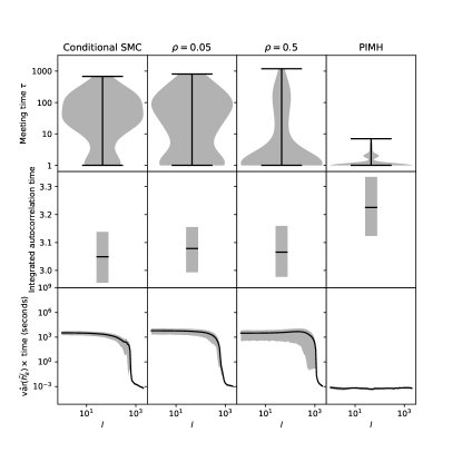
Figure 1 shows that meeting times are lowest for Algorithm 6 with PIMH while mixing of the outer MCMC step is best with conditional SMC. A mixed set-up with , aimed at a trade-off between these extremes, has coupling and mixing performance in between and . Nonetheless, criterion ‘’, defined in the second paragraph of Section 5, is slightly lower for than for conditional SMC only for values of where PIMH is superior, a pattern observed also for scenarios described in Appendix D. The criterion is lowest for conditional SMC owing to its better mixing but only if Algorithm 6 is run for sufficiently more iterations than the largest meeting times. Finally, we compare our methodology with the coupled HMC of Heng and Jacob (2019) in Appendix C showing the coupled particle MCMC is more efficient in the scenario considered, though it must be noted that HMC is not well suited for multimodal targets.
5.2 Horseshoe regression
Background
Biswas et al. (2021) recently proposed a coupled MCMC for horseshoe regression (Carvalho et al., 2009). This section compares the coupling and its resulting unbiased estimation with the proposed coupled particle MCMC in Algorithm 6.
We consider the standard likelihood for linear regression with a -dimensional vector of observations, a design matrix and the error variance. The main object of inference is the -dimensional coefficient vector . The horseshoe prior on is one of the most popular global-local shrinkage priors for state-of-the-art Bayesian variable selection (Bhadra et al., 2019). It is defined by independently for where is a global precision parameter with prior and is a local precision parameter with prior independently for . Here, denotes the standard half-Cauchy distribution. That is, if , then the density of is for and zero otherwise.
We follow the simulation set-up of Biswas et al. (2021, Section 3). The gamma prior completes the Bayesian model specification. The elements of the matrix are sampled independently from the standard Gaussian distribution. We draw for some true and true error variance . We set , , , for and for .
Coupled particle MCMC for horseshoe regression
We construct our inner MCMC steps by making use of Algorithm 1 from Biswas et al. (2021). Here, since the MCMC provides a Markov chain on these parameters jointly. Our method requires an inner MCMC step that is invariant w.r.t. , e.g., Step 2c of Algorithm 2. Here, equals with , and replaced by , and , respectively. Thus, the required inner MCMC for follows by carrying out these replacements in the inner MCMC step as developed for the full posterior .
The scalar statistics used for determining the number of MCMC steps are the log-likelihood function, that is , and the number of elements in with absolute value greater than , . The latter is interpreted as the number of variables chosen by the model. Algorithm 1 produces for all . This confirms the effectiveness of the inner MCMC algorithm borrowed from Biswas et al. (2021), which is accompanied by favourable theoretical properties as per Biswas et al. (2021, Section 2.2). We compare the estimation of the posterior expectation of , , obtained from different algorithms.
Results
We compare the results from coupled particle MCMC (Algorithm 6) with and using particles to the two-scale coupling of Biswas et al. (2021, Section 3.2) which provides a direct coupling of an MCMC algorithm that we use as the inner MCMC step. Algorithm 6 with uses this same coupling of the inner MCMC when calling Algorithm 4. We do not present the results for smaller values of as they are not competitive due to too large meeting times. The three coupled MCMCs are run times each for iterations. Figure 2 presents the results analogously to Figure 1.

Coupled particle MCMC meets in fewer iterations than the coupled MCMC from Biswas et al. (2021). Nonetheless, coupled particle MCMC takes more computation time to achieve the same estimation accuracy. One reason for this is the mixing of the coupled MCMC as shown in Figure 2 with a much higher integrated autocorrelation time for coupled particle MCMC. Another reason is that the computational cost of the outer particle MCMC step in Algorithm 6 is much higher than that of a single inner MCMC step. This increased cost of particle methods could be alleviated by parallelizing across particles if the main concern is elapsed real time rather than cumulative CPU time across CPU cores. More generally, effective direct couplings of (inner) MCMC, like the method from Biswas et al. (2021), would often be superior if available, as any improved coupling through SMC methods does not justify their added cost. On the other hand, coupled particle MCMC can be useful when effective direct coupling is not available. The results for ‘’ show that it is not sufficient to only consider meeting times when assessing coupled MCMC for unbiased estimation if the MCMC algorithms compared differ in mixing or computational cost.
Figure 2 suggests that conditional SMC mixes better than PIMH but results in a worse coupling of the outer MCMC. Here, the improvement over PIMH in mixing does not outweigh the worse coupling of conditional SMC and the associated variance of the bias correction term at outer MCMC iterations. For sufficiently large, the relative contribution of the bias correction term would vanish resulting in lower ‘’ for conditional SMC than for PIMH, though such might not be computationally feasible.
6 Application: Gaussian graphical models
6.1 Model
We consider Gaussian graphical models (Dempster, 1972; Lauritzen, 1996) as an example of a complex posterior on discrete spaces. Coupling of MCMC kernels on the original non-extended space appears highly challenging. In general, generation of unbiased estimators for posterior expectations in this context is a major undertaking, and it is attempted, to the best of our knowledge, for the first time in this work. We allow the graphs to be non-decomposable, and present methodology that sidesteps approximation of intractable normalising constants.
The object of inference is an undirected graph defined by a set of nodes , , and a set of edges . As in Lenkoski (2013), we slightly abuse notation and write for , i.e. when vertices and are connected in . We aim to infer given an data matrix with independent rows distributed according to for a precision matrix , where is the set of symmetric, positive-definite matrices. Graph constrains in that if . Thus, , where is the cone of matrices with for .
Under the notation in Section 3, we have , . Notice that we are required to include into as only then is analytically available. We get that is equal to , where is the scatter matrix and the trace inner product. A conjugate prior for conditional on is the -Wishart distribution (Roverato, 2002) with density
parametrised by and a positive-definite rate matrix . The normalising constant does not have an analytical form for general non-decomposable (Uhler et al., 2018). We henceforth choose in agreement with previous work (Jones et al., 2005; Lenkoski, 2013; Tan et al., 2017). Due to conjugacy, where . Since the objective is inference on , one would like to compute the posterior
| (3) | ||||
with the prior on .
As the normalising constant is not analytically available in general, some approximation is required. Standard approaches apply Monte Carlo or Laplace approximation of (Atay-Kayis and Massam, 2005; Tan et al., 2017). Recent work avoids approximation of normalising constants via careful MCMC constructions. See Wang and Li (2012); Cheng and Lenkoski (2012); Lenkoski (2013); Hinne et al. (2014). Our methodology falls in this latter direction of research. Compared to Wang and Li (2012); Cheng and Lenkoski (2012), our MCMC samples directly from -Wishart laws, rather than preserving them, to improve mixing. Our MCMC sampler is very similar to the one in Lenkoski (2013), with the exception of sampling elements of the precision matrices directly from the full conditional distribution, rather that applying a Metropolis-within-Gibbs step.
We use a size-based prior (Armstrong et al., 2009, Section 2.4) for . That is, is the induced marginal of a joint prior distribution on and the number of edges such that the prior on given is uniform, . For , we choose a truncated geometric distribution with success probability , i.e. , . This choice completes the prior specification for and induces sparsity. The success probability is such that the mean of the non-truncated geometric law equals the number of vertices . Prior elicitation based on the sparsity constraint that the prior mean of equals has also been used with independent-edge priors (Jones et al., 2005, Section 2.4).
6.2 Further algorithmic specifications
We derive an inner MCMC step in Appendix E to apply Algorithm 6 to Gaussian graphical models. Here, we further detail how we use Algorithm 6.
Rejection sampling with
We set and resort to rejection sampling with the prior as proposal to sample from in Step 1 of Algorithm 2. This reduces the computational cost for the overall SMC algorithm considerably in our applications, due to the prior being diffuse: the inner MCMC step (Algorithm 10) changes at most one edge of the graph in each step such that a large number of steps are required for effective diversification of particles for small for which . This implementation of the MCMC steps then dominates the computational cost. Setting induces a larger and a much smaller .
The maximum likelihood estimate of the precision is . So, the acceptance probability of the rejection sampler follows as
We choose to achieve an acceptance rate of . Specifically, we draw particles from the prior and set to the largest value such that of these particles are accepted.
PIMH vs conditional SMC
The main challenge for the class of Gaussian graphical models is the effective coupling of the outer MCMC chain so that the size of the meeting times is not too large. Following the discussion in Section 5, PIMH yields smaller than conditional SMC. We therefore use Algorithm 6 with here. Even so, some chains fail to couple (Section 6.4), suggesting that lower values of would result in impracticably large meeting times.
6.3 Data description
We apply the Gaussian graphical models on a set of metabonomic data. The sample consists of six-year-old children from the Growing Up in Singapore Towards healthy Outcomes (GUSTO) study (Soh et al., 2014). Measurements are taken from blood serum samples via nuclear magnetic resonance to obtain metabolic phenotypes. Specifically, the levels of certain metabolites, which are low-molecular-weight molecules involved in metabolism, are measured. Examples of metabolites are cholesterol, fatty acids and glucose. See Soininen et al. (2009) for a description of the measurement process. We focus on a set of 35 metabolites. Thus, the data matrix consists of metabolite levels. We quantile normalise the metabolites such that they marginally follow a standard Gaussian distribution.
6.4 Results
The statistics used to determine the number of inner MCMC steps are the log-likelihood and the number of edges . The adaptation results in temperatures with varying from 1 to 14 and a mean of 6 for , whereas . Indeed, having ensures that the tempered posterior is further away from the uninformative prior such that the number of MCMC steps for sufficient diversification of particles is limited.
Algorithm 6 is run for MCMC steps with particles, until the chains meet or when the time budget is up, whichever happens first. We do this repeatedly across 16 CPU cores simultaneously and independently. Our time budget is 72 hours. This results in 30 finished runs of Algorithm 6 and 16 incomplete runs that are cut short due to running out of time. The failure to meet suggests that this posterior is at the limit of what is computationally feasible with the version and numerical execution of coupled particle MCMC used in this work. We discard the incomplete runs which introduces a bias, though this bias decays exponentially with the time budget as discussed in Section 3.3 of Jacob et al. (2020b). Of the 30 finished runs, 19 meet in step and the largest observed is .
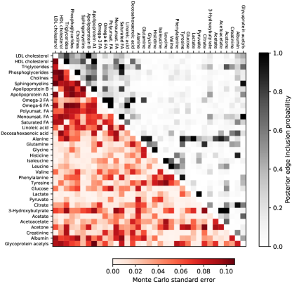

We use these runs to obtain multiple unbiased estimates based on (2) with and where is chosen to estimate the posterior edge inclusion probabilities, i.e. the posterior probability of an edge being included in the graph . Figure 3 shows the estimates. Since they result from averaging independent and unbiased estimators, we can also estimate their Monte Carlo error. Figure 3 confirms that the chosen time budget is sufficient to achieve a usable posterior approximation with the standard errors maxing out at 0.11. Appendix G compares these probabilities with estimates from running SMC once with a large number of particles. Figure 4 contains the median probability graph, i.e. the graph which includes edges with a posterior inclusion probability greater than .
7 Discussion
In this work we propose a coupled particle MCMC methodology that can yield effective unbiased posterior approximation and enjoys attractive theoretical properties. Gaussian graphical models provide an example where a good coupling of the MCMC is hard while coupled particle MCMC produces Markov chains that tend to couple quickly. A major contribution of this manuscript is to embed recent developments in the field into a general procedure, building a complete and flexible computational strategy within the area of unbiased MCMC. Moreover, we investigate the performance of the proposed coupled particle MCMC in challenging settings. The paper places itself within an active and recent area of research, and our numerical applications (horseshoe regression, Gaussian graphical models) constitute far more complex examples than those typically considered in the literature on unbiased estimation in state-space models. Furthermore, it is applicable, in an automatic way (in principle), to a broad class of posterior distributions, while existing literature often focuses on particular classes of targets.
The empirical results show that using PIMH instead of conditional SMC in Algorithm 6, as controlled by the parameter , provides a trade-off between coupling and MCMC mixing with conditional SMC corresponding with better mixing. Thus, conditional SMC results in the most efficient unbiased estimates for number of iterations sufficiently large, though computing them might be impracticable due to too large meeting times. Then, PIMH provides a computationally more feasible alternative. Whether conditional SMC is feasible can be determined by preliminary and potentially incomplete runs of Algorithm 6. Generally, conditional SMC results in fewer replicate unbiased estimates, which might prevent optimal use of available computing resources (e.g. parallelisation) as well as lead to less reliable estimates of Monte Carlo error. We additionally consider a mixture of PIMH and conditional SMC. We do not find it to be empirically superior in the scenarios considered and existing theoretical results do not immediately apply. Such mixture is similar in spirit to the use of both a coupled Metropolis-Hastings step and a coupled HMC step in Heng and Jacob (2019) where that mixture also provides a trade-off between coupling and MCMC mixing.
Major empirical and theoretical improvements in coupling have been reported for the ancestral and backward sampling modifications to the standard version of conditional SMC (Chopin and Singh, 2015; Jacob et al., 2020a; Lee et al., 2020). For instance, Lee et al. (2020, Theorem 11) show that the one-step meeting probability analysed in Proposition 1 does not vanish if for conditional SMC with backward sampling. Unfortunately, these modifications can usually not be used in our scenario as the transition densities in the Feynman-Kac model resulting from taking inner MCMC steps are often intractable.
The use of SMC adds computational cost compared to running MCMC by itself. For instance, a single step in the outer MCMC defined by PIMH or conditional SMC involves inner MCMC steps. This extra computational cost is amenable to parallelization due to the embarrassingly parallel nature of the particles in SMC. Moreover, the extra computational effort results in more accurate Monte Carlo estimates due to Rao-Blackwellization across the particles. One of the main contributions of this work is to gain further insights into these novel computational strategies. For instance, the numerical experiments in Section 5 indicate that the shape of the posterior at hand determines the efficiency in the performance of SMC-based coupling against alternative approaches.
Acknowledgements.
We thank the referees for many useful suggestions that helped to greatly improve the content of the paper. This version of the article has been accepted for publication, after peer review (when applicable) but is not the Version of Record and does not reflect post-acceptance improvements, or any corrections. The Version of Record is available online at: \urlhttp://dx.doi.org/10.1007/s11222-022-10093-3. Use of this Accepted Version is subject to the publisher’s Accepted Manuscript terms of use \urlhttps://www.springernature.com/gp/open-research/policies/accepted-manuscript-terms.References
- Andrieu et al. (2010) Andrieu C, Doucet A, Holenstein R (2010) Particle Markov chain Monte Carlo methods. Journal of the Royal Statistical Society: Series B (Statistical Methodology) 72(3):269–342
- Andrieu et al. (2018) Andrieu C, Lee A, Vihola M (2018) Uniform ergodicity of the iterated conditional SMC and geometric ergodicity of particle Gibbs samplers. Bernoulli 24(2):842–872
- Armstrong et al. (2009) Armstrong H, Carter CK, Wong KFK, Kohn R (2009) Bayesian covariance matrix estimation using a mixture of decomposable graphical models. Statistics and Computing 19(3):303–316
- Atay-Kayis and Massam (2005) Atay-Kayis A, Massam H (2005) A Monte Carlo method for computing the marginal likelihood in nondecomposable Gaussian graphical models. Biometrika 92(2):317–335
- Bhadra et al. (2019) Bhadra A, Datta J, Polson NG, Willard B (2019) Lasso meets horseshoe: A survey. Statistical Science 34(3):405–427
- Biswas et al. (2021) Biswas N, Bhattacharya A, Jacob PE, Johndrow JE (2021) Coupled Markov chain Monte Carlo for high-dimensional regression with Half-t priors. arXiv:2012.04798v2
- Carvalho et al. (2009) Carvalho CM, Polson NG, Scott JG (2009) Handling sparsity via the horseshoe. In: van Dyk D, Welling M (eds) Proceedings of the Twelth International Conference on Artificial Intelligence and Statistics, PMLR, Hilton Clearwater Beach Resort, Clearwater Beach, Florida USA, Proceedings of Machine Learning Research, vol 5, pp 73–80
- Cheng and Lenkoski (2012) Cheng Y, Lenkoski A (2012) Hierarchical Gaussian graphical models: Beyond reversible jump. Electronic Journal of Statistics 6:2309–2331
- Chopin and Papaspiliopoulos (2020) Chopin N, Papaspiliopoulos O (2020) An Introduction to Sequential Monte Carlo. Springer International Publishing
- Chopin and Singh (2015) Chopin N, Singh SS (2015) On particle Gibbs sampling. Bernoulli 21(3):1855–1883
- Del Moral (2004) Del Moral P (2004) Feynman-Kac Formulae: Genealogical and Interacting Particle Systems with Applications. Springer, New York
- Del Moral et al. (2006) Del Moral P, Doucet A, Jasra A (2006) Sequential Monte Carlo samplers. Journal of the Royal Statistical Society: Series B (Statistical Methodology) 68(3):411–436
- Dempster (1972) Dempster AP (1972) Covariance selection. Biometrics 28(1):157
- Dobra et al. (2011) Dobra A, Lenkoski A, Rodriguez A (2011) Bayesian inference for general Gaussian graphical models with application to multivariate lattice data. Journal of the American Statistical Association 106(496):1418–1433
- Glynn and Rhee (2014) Glynn PW, Rhee CH (2014) Exact estimation for Markov chain equilibrium expectations. Journal of Applied Probability 51(A):377–389
- Godsill (2001) Godsill SJ (2001) On the relationship between Markov chain Monte Carlo methods for model uncertainty. Journal of Computational and Graphical Statistics 10(2):230–248
- Heng and Jacob (2019) Heng J, Jacob PE (2019) Unbiased Hamiltonian Monte Carlo with couplings. Biometrika 106(2):287–302
- Hinne et al. (2014) Hinne M, Lenkoski A, Heskes T, van Gerven M (2014) Efficient sampling of Gaussian graphical models using conditional Bayes factors. Stat 3(1):326–336
- Jacob et al. (2020a) Jacob PE, Lindsten F, Schön TB (2020a) Smoothing with couplings of conditional particle filters. Journal of the American Statistical Association 115(530):721–729
- Jacob et al. (2020b) Jacob PE, O’Leary J, Atchadé YF (2020b) Unbiased Markov chain Monte Carlo methods with couplings. Journal of the Royal Statistical Society: Series B (Statistical Methodology) 82(3):543–600
- Jasra et al. (2010) Jasra A, Stephens DA, Doucet A, Tsagaris T (2010) Inference for Lévy-driven stochastic volatility models via adaptive sequential Monte Carlo. Scandinavian Journal of Statistics 38(1):1–22
- Jasra et al. (2017) Jasra A, Kamatani K, Law KJH, Zhou Y (2017) Multilevel particle filters. SIAM Journal on Numerical Analysis 55(6):3068–3096
- Jones et al. (2005) Jones B, Carvalho C, Dobra A, Hans C, Carter C, West M (2005) Experiments in stochastic computation for high-dimensional graphical models. Statistical Science 20(4):388–400
- Kantas et al. (2014) Kantas N, Beskos A, Jasra A (2014) Sequential Monte Carlo methods for high-dimensional inverse problems: A case study for the Navier–Stokes equations. SIAM/ASA Journal on Uncertainty Quantification 2(1):464–489
- Lauritzen (1996) Lauritzen SL (1996) Graphical Models. Oxford Statistical Science Series, The Clarendon Press, Oxford University Press, New York
- Lee et al. (2020) Lee A, Singh SS, Vihola M (2020) Coupled conditional backward sampling particle filter. Annals of Statistics 48(5):3066–3089
- Lenkoski (2013) Lenkoski A (2013) A direct sampler for G-Wishart variates. Stat 2(1):119–128
- Middleton et al. (2019) Middleton L, Deligiannidis G, Doucet A, Jacob PE (2019) Unbiased smoothing using particle independent Metropolis-Hastings. In: Chaudhuri K, Sugiyama M (eds) Proceedings of Machine Learning Research, PMLR, Proceedings of Machine Learning Research, vol 89, pp 2378–2387
- Murray et al. (2006) Murray I, Ghahramani Z, MacKay DJC (2006) MCMC for doubly-intractable distributions. In: Proceedings of the Twenty-Second Conference on Uncertainty in Artificial Intelligence, AUAI Press, Arlington, Virginia, USA, UAI’06, p 359–366
- Rosenthal (1997) Rosenthal JS (1997) Faithful couplings of Markov chains: Now equals forever. Advances in Applied Mathematics 18(3):372–381
- Roverato (2002) Roverato A (2002) Hyper inverse Wishart distribution for non-decomposable graphs and its application to Bayesian inference for Gaussian graphical models. Scandinavian Journal of Statistics 29(3):391–411
- Soh et al. (2014) Soh SE, Tint MT, Gluckman PD, Godfrey KM, Rifkin-Graboi A, Chan YH, Stünkel W, Holbrook JD, Kwek K, Chong YS, Saw SM, the GUSTO Study Group (2014) Cohort profile: Growing up in Singapore towards healthy outcomes (GUSTO) birth cohort study. International Journal of Epidemiology 43(5):1401–1409
- Soininen et al. (2009) Soininen P, Kangas AJ, Würtz P, Tukiainen T, Tynkkynen T, Laatikainen R, Järvelin MR, Kähönen M, Lehtimäki T, Viikari J, Raitakari OT, Savolainen MJ, Ala-Korpela M (2009) High-throughput serum NMR metabonomics for cost-effective holistic studies on systemic metabolism. The Analyst 134(9):1781
- Statisticat, LLC. (2020) Statisticat, LLC (2020) LaplacesDemon: Complete Environment for Bayesian Inference. R package version 16.1.4
- Tan et al. (2017) Tan LSL, Jasra A, De Iorio M, Ebbels TMD (2017) Bayesian inference for multiple Gaussian graphical models with application to metabolic association networks. The Annals of Applied Statistics 11(4):2222–2251
- Uhler et al. (2018) Uhler C, Lenkoski A, Richards D (2018) Exact formulas for the normalizing constants of Wishart distributions for graphical models. The Annals of Statistics 46(1):90–118
- Wang and Li (2012) Wang H, Li SZ (2012) Efficient Gaussian graphical model determination under G-Wishart prior distributions. Electronic Journal of Statistics 6(0):168–198
Appendix A Systematic resampling
Algorithms 7 through 9 detail the systematic resampling methods used for the empirical results derived from Algorithm 6. They involve the floor function denoted by , i.e., is the largest integer for which .
Input: Probability vector and .
-
1.
Compute the cumulative sums , .
-
2.
Let .
-
3.
For ,
-
(a)
While , do .
-
(b)
Let and .
-
(a)
Output: A vector of random indices such that, if the input follows , then the expectation of the frequency of any index equals .
Input: Probability vector .
-
1.
Compute and sample
-
2.
Obtain a vector of indices by running Algorithm 7 with and as input.
-
3.
Draw uniformly from all cycles of that yield .
Output: A vector of random indices with .
Input: Probability vectors , .
-
1.
Generate and by running the first two steps of Algorithm 8 with and as input, respectively, using the same random numbers for each.
-
2.
Construct a joint probability distribution on the cycles and of and for which such that the marginal distributions are uniform:
-
(a)
Calculate the overlap for each pair of cycles with .
-
(b)
Iteratively assign the largest probability afforded by the constraint of uniform marginals to the pair with the highest overlap.
-
(a)
-
3.
Draw and from this joint distribution on cycles of and .
Output: Vectors , of random indices with .
Appendix B Proofs for Section 4
Our results derive from Lee et al. (2020). They consider a smoothing set-up which maps to our context of approximating a general posterior using adaptive SMC. Specifically, their target density is (Lee et al., 2020, Equation 1)
| (4) |
In our context, the term is a tempered posterior, the term a tempered likelihood, the density of the Markov transition starting at resulting from the MCMC steps which are invariant w.r.t. in Step 2c of Algorithm 2 for , a tempered likelihood for , and a tempered likelihood. Then, the coupled conditional particle filter in Algorithm 2 of Lee et al. (2020) reduces to the coupled conditional SMC in our Algorithm 4. Thus, the results in Lee et al. (2020) apply to Algorithm 4.
B.1 Proof of Proposition 1
Since does not depend on , we can write for as in Section 2 of Lee et al. (2020). Assumption 1, that is bounded, implies that is bounded for , which is Assumption 1 in Lee et al. (2020). Therefore, Theorem 8 of Lee et al. (2020) provides
Part (iii) follows similarly to the proof for Theorem 10(iii) of Lee et al. (2020): We have for . Therefore,
where the last equality follows from the geometric series formula
for .
Part (iii) implies Part (ii). ∎
B.2 Proof of Proposition 2
Theorem 10 of Lee et al. (2020) provides results for a statistic that we denote by . Consider defined by where is our statistic of interest. Then, is bounded by Assumption 2. The marginal distribution of under the density on in (4) is our posterior of interest . Consequently, the results for in Theorem 10 of Lee et al. (2020) provide the required results for . ∎
Appendix C Comparison with coupled HMC
The coupled HMC method of Heng and Jacob (2019) provides an alternative to coupled particle MCMC for unbiased posterior approximation if the posterior is amenable to HMC. The latter typically requires and that the posterior is continuously differentiable. Here, we apply coupled HMC to the posterior considered in Section 5.1 with a slight modification to make it suitable for HMC: the uniform prior over the hypercube is replaced by the improper prior for to ensure differentiability. The set-up of coupled HMC follows Section 5.2 of Heng and Jacob (2019) with the following differences. The leap-frog step size is set to 0.1 instead of 1 as the resulting MCMC failed to accept with the latter. We do not initialize both chains independently but instead set as in Algorithm 6 since we found that this change reduces meeting times. We use code from \urlhttps://github.com/pierrejacob/debiasedhmc to implement the method from Heng and Jacob (2019).

Figure 5 presents the results analogously to Figure 1. In terms of number of iterations, coupled HMC mixes worse and takes longer to meet than coupled particle MCMC. These increases are not offset by a lower computational cost per iteration. An important caveat here is that computation time depends on the implementation, and here coupled HMC is implemented using an R package and coupled particle MCMC in Python.
Appendix D Additional simulations studies
Here, we provide some further simulation studies where the set-up is the same as in Section 5.1 except for the following. We consider a probability of PIMH of in addition to the other values of , the maximum is and the number of repetitions is . Figure 8 considers different number of particles of . Figure 9 varies the dimensionality of the parameter where we use the true values and for and , respectively, based on the set-up in Middleton et al. (2019, Appendix B.2). Additionally, Figure 9b uses independent inner MCMC steps across both chains except for that the MCMC step is faithful to any coupling. This contrasts with Section 5.1 which uses a common random number coupling for the Metropolis-Hastings inner MCMC step.
A higher number of particles results in shorter meeting times. Criterion ‘’ is lowest for larger , though beyond a certain , not much improvement is gained. Jacob et al. (2020a) reach a similar conclusion when varying for coupled conditional particle filters.
Performance deteriorates with increasing dimensionality , especially for smaller values of . For (Figure 9d), the chains even often fail to meet within the maximum number of iterations of 2,000 considered for . We also see such lack of coupling in Figure 9b for , suggesting that the coupling of the inner MCMC is important for good performance when working with coupled conditional SMC. This is despite the fact that the theoretical results in Section 4 do not depend on the quality of the coupling of the inner MCMC.
For certain values of , using away from 0 or 1 is competitive with conditional SMC or PIMH in terms of ‘’ although not notably better than using just one of them. The benefit of a mixture versus using only conditional SMC in terms of coupling is highlighted in Figure 9b where the inner MCMC is uncoupled.
Appendix E Inner MCMC step for Gaussian graphical models
We set up an MCMC step with as invariant distribution. The corresponding MCMC step for the tempered density , , required for Algorithm 6, follows by replacing and by and , respectively, as . We make use of the algorithm for sampling from a -Wishart law introduced in Lenkoski (2013, Section 2.4). Thus, we can sample from . It remains to derive an MCMC transition that preserves , as samples of can be extended to by generating .
We consider the double reversible jump approach from Lenkoski (2013) and apply the node reordering from Cheng and Lenkoski (2012, Section 2.2) to obtain an MCMC step with no tuning parameters. The MCMC step is a Metropolis-Hastings algorithm on an enlarged space that bypasses the evaluation of the intractable normalisation constants and in the target distribution (3). It is a combination of ideas from the PAS algorithm of Godsill (2001), which avoids the evaluation of , and the exchange algorithm of Murray et al. (2006), which sidesteps evaluation of . We will give a brief presentation of the MCMC kernel that we are using as it does not coincide with approaches that have appeared in the literature.
To attain the objective of suppressing the normalising constants in the method, one works with a posterior on an extended space, defined via the directed acyclic graph in Figure 6. The left side of the graph gives rise to the original posterior . Denote by the proposed graph, with law . Lenkoski (2013) chooses a pair of vertices in , , at random and applies a reversal, i.e. if and only if . The downside is that the probability of removing an edge is proportional to the number of edges in , which is typically small. Instead, we consider the method in Dobra et al. (2011, Equation A.1) that also applies the reversal, but chooses so that the probabilities of adding and removing an edge are equal.
We reorder the nodes of and so that the edge that has been altered is , similarly to Cheng and Lenkoski (2012, Section 2.2). Given , the graph in Figure 6 contains a final node that refers to the conditional distribution of which coincides with the -Wishart prior . Consider the upper triangular Cholesky decomposition of so that . Let . We work with the map . We apply a similar decomposition for , and obtain the map .
We can now define the target posterior on the extended space as
| (5) |
Given a graph , the current state on the extended space comprises of
| (6) |
with , and , obtained from the Cholesky decomposition of the precision matrices , , respectively. Note that the rows and columns of , have been accordingly reordered to agree with the re-arrangement of the nodes we describe above. Consider the scenario with the proposed graph having one more edge than . Given the current state in (6), the algorithm proposes a move to the state
| (7) |
The value is sampled from the conditional law of .
We provide here some justification for the above construction. The main points are the following: (i) the proposal corresponds to an exchange of , coupled with a suggested value for the newly ‘freed’ matrix element ; (ii) from standard properties of the general exchange algorithm, switching the position of will cancel out the normalising constants of the -Wishart prior from the acceptance probability; (iii) the normalising constants of the -Wishart posterior never appear, as the precision matrices are not integrated out.
Appendix F derives that
| (8) |
This avoids the tuning of a step-size parameter arising in the Gaussian proposal of Lenkoski (2013, Section 3.2). The variable is not free, due to the edge assumed being removed, and is given as (Roverato, 2002, Equation 10)
The acceptance probability of the proposal is given in Step 6 of the complete MCMC transition shown in Algorithm 10 for exponent . In the opposite scenario when an edge is removed from , then, after again re-ordering the nodes, the proposal is sampled from
whereas we fix . The corresponding acceptance probability for the proposed move is again as in Step 6 of Algorithm 10, but now for .
Input: Graph .
-
1.
-
(a)
If is complete or empty, sample , , uniformly from the edges in or the edges not in , respectively.
-
(b)
Else, sample , , as follows: w.p. , uniformly from the edges in ; w.p. , uniformly from the edges not in .
-
(a)
-
2.
Reorder the nodes in so that the -th and -th nodes become the -th and -th nodes, respectively. Rearrange and accordingly.
-
3.
Let be as except for edge , with if and only if .
-
4.
Sample , . Compute the corresponding upper triangular Cholesky decompositions , .
-
5.
Fix and .
-
(a)
If , sample the proposal
and set .
-
(b)
If , sample the proposal
and set .
-
(a)
-
6.
Accept proposed move from to state w.p. , for equal to
for and . Here, (resp. ) denotes the precision with upper triangular Cholesky decomposition given by the synthesis of (resp. ), and if , else .
- 7.
Output: MCMC update for graph such that the invariant distribution is the target posterior .
Appendix F Proposal for precision matrices
This derivation is similar to Appendix A of Cheng and Lenkoski (2012). Assume that the edge is in the proposed graph but not in . The prior on follows from Equation 2 of Cheng and Lenkoski (2012) as
The likelihood is
Here, does not depend on since . Combining the previous two displays thus yields . Dropping terms not involving yields (8).
Appendix G Comparison with SMC for the metabolite application
We compare the results in Figure 3 with those from running the SMC in Algorithm 2 with a large number of particles . Comparing Figures 3 and 7 shows that the results are largely the same. The edge probabilities for which they differ substantially are harder to estimate according to the Monte Carlo standard errors from coupled particle SMC in Figure 3.