Unavoidable emergent biaxiality in chiral molecular-colloidal hybrid liquid crystals
Abstract
Chiral nematic or cholesteric liquid crystals (LCs) are chiral mesophases with long-ranged orientational order featuring a quasi-layered periodicity imparted by a helical director configuration but lacking positional order. Doping molecular cholesteric LCs with thin colloidal rods with a large length-to-width ratio or disks with a large diameter-to-thickness ratio adds another level of complexity to the system because of the interplay between weak surface anchoring boundary conditions and bulk-based elastic distortions around the particle-LC interface. By using colloidal disks and rods with different geometric shapes and boundary conditions, we demonstrate that these anisotropic colloidal inclusions exhibit biaxial orientational probability distributions, where they have tendencies to orient with the long rod axes and disk normals perpendicular to the helix axis, thus imparting strong local biaxiality on the hybrid cholesteric LC structure. Unlike the situation in non-chiral hybrid molecular-colloidal LCs, where biaxial order emerges only at modest to high volume fractions of the anisotropic colloidal particles, above a uniaxial-biaxial transition concentration, the orientational probability distribution of colloidal inclusions immersed in chiral nematic hosts are unavoidably biaxial even at vanishingly low particle volume fractions. In addition, the colloidal inclusions induce local biaxiality in the molecular orientational order of the LC host medium, which enhances the weak biaxiality of the LC in a chiral nematic phase coming from the symmetry breaking caused by the presence of the helical axis. With the help of analytical modeling and computer simulations based on minimizing the Landau de Gennes free energy of the host LC around the colloidal inclusions, we explain our experimental findings and conclude that the biaxial order of chiral molecular-colloidal LCs is strongly enhanced as compared to both achiral molecular-colloidal LCs and molecular cholesteric LCs and is rather unavoidable.
I Introduction
Since the experimental discovery of chiral nematic liquid crystals (LCs) over 150 years ago planer1861notiz ; reinitzer1888beitrage , LC mesophases featuring chirality and long-range orientational order have been the focus of many research studies. The fundamental studies of geometry and topology of chiral nematic LCs as model systems provide extensive insights into physics principles associated with experimentally less accessible systems like particle physics or cosmology wu2022hopfions ; ackerman2014two ; tai2020surface ; volovik2001superfluid ; bowick1994cosmological ; meng2023topological ; smalyukh2020knots ; smalyukh2018liquid ; kamada2022chiral ; chaikin1995principles , in addition to their technological application in electro-optics and displays. On the other hand, biaxial nematic mesophases have been highly sought-after in soft matter systems since their first theoretical consideration in 1970 freiser1970ordered . However, even in a soft-matter system with strongly biaxial building blocks such as brick-shaped molecules, biaxiality was experimentally elusive and hard to unambiguously demonstrate in equilibrium states. Recent reports of the experimental discovery of biaxial nematic order include observations in micellar and molecular LCs formed by amphiphilic and bent-core molecules, respectively yu1980observation ; tschierske2010biaxial , and also colloidal dispersion of highly anisotropic particles immersed in molecular LC hosts, so-called hybrid molecular-colloidal nematics liu2016 ; mundoor2021 ; mundoor2018 . The interplay between chirality and biaxiality in orientational order has been intensively studied for LC systems priest1974biaxial ; kroin1989chirality ; bunning1986effect ; harris1997microscopic ; dussi2016entropy ; dhakal2011chirality ; longa1994biaxiality ; canevari2015biaxiality ; harris1999molecular ; lubensky1998chirality . It has been concluded that cholesteric twisted alignment and biaxial order of LC molecules amplify each other and that a chiral twist configuration cannot be observed without building blocks featuring a certain degree of biaxiality in their orientational distributions at the molecular level. However, for purely molecular systems, the chirality-enhanced biaxiality of the molecular distribution was predicted and experimentally found to be rather weak priest1974biaxial ; kroin1989chirality ; bunning1986effect ; harris1997microscopic ; dussi2016entropy ; dhakal2011chirality ; longa1994biaxiality ; canevari2015biaxiality , scaling as according to the prediction by Priest and Lubensky for single-component molecular LCs priest1974biaxial (here , is the helical pitch of the chiral nematic and the molecular length). To date, to the best of our knowledge, there are no experimental or theoretical considerations of how the biaxiality of the orientational distribution of anisotropic colloidal particles could interplay with the chirality of the nematic host in hybrid molecular-colloidal LC systems.

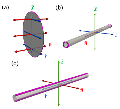
In this work, we demonstrate an unavoidably biaxial orientation probability distribution for uniaxial colloidal particles dispersed in a weakly chiral molecular host, which is rather unexpected. We report strongly enhanced biaxial order in the orientational distribution probability for colloidal rods scaling as , where the length of the colloidal particles is in the micron range, more than 3 orders of magnitude larger than that of LC molecules, albeit still an order of magnitude or so smaller than the pitch . The geometry of the cholesteric LC is described by three non-polar, orthogonal director fields [Fig. 1]: molecular director field representing the local average molecular alignment, the helical axis field along which rotates, and the third field kleman1989defects ; lavrentovich2001cholesteric . Here, the helicoidal configuration with a mutually perpendicular molecular frame and helical pitch is hardly perturbed by the introduction of thin colloidal disks or rods in view of their low concentration and weak surface anchoring boundary conditions. The colloidal particles are uniaxial on their own with high aspect ratios, and their orientations are well-controlled by pre-designed boundary conditions. The biaxiality of the colloidal orientational distribution is found to exceed values known for biaxiality on the molecular scale in cholesteric LCs and in nematic molecular colloidal-molecular hybrid systems, despite the low colloidal concentration and weak chirality of the molecular host. In cases where the colloids align along the axis, the biaxiality is found to be more pronounced than when they are aligned along the molecular director . Furthermore, the molecular biaxiality of the LC host medium is further boosted by surface anchoring-induced distortions at the edges of the colloidal particles. In contrast to the orientational distribution of colloidal inclusions in nematic hybrid molecular-colloidal LCs, in which biaxial order emerges only at modest to high volume fractions of anisotropic colloidal particles mundoor2021 , the orientational probability distribution of colloidal inclusions in chiral nematic hosts is unavoidably biaxial even at very low colloidal volume fractions. In turn, colloidal inclusions impart local biaxiality onto the molecular orientational distributions of the LC host medium, which enhances the weak biaxial order of the LC in a chiral nematic phase due to the symmetry breaking caused by the presence of the helical axis. With the help of computer simulations based on minimizing the Landau de Gennes free energy of the LC host around the colloidal inclusions [Fig. 2], we explain our experimental findings and conclude that the biaxial order of chiral molecular-colloidal LCs is enhanced compared to that of both nematic molecular-colloidal and cholesteric molecular counterparts. We demonstrate that the interplay between chirality and biaxiality in hybrid molecular-colloidal LCs is stronger than that in purely molecular or colloidal systems and that the biaxial symmetry of the orientational distributions of the anisotropic colloids is a universal feature. Finally, we discuss how our findings may allow for expanding the use of chiral molecular-colloidal LCs as model systems in studies of nonabelian defect lines and topological solitons hosted by states of matter with high-dimensional order parameter spaces.
II Methods and Techniques
II.1 Synthesis of colloidal disks and rods
Disk or rod-shaped :Yb/Er particles are synthesized following the hydrothermal synthesis methods described in detail elsewhere mundoor2021 ; mundoor2018 ; mundoor2019electrostatically ; wang2007controlled ; yang2012one . Precursors and solvents used for the synthesis of colloidal particles are of analytical grade and used without additional purifications, and they are bought from Sigma Aldrich if not specified otherwise. To synthesize nanodisks, 0.7 g of sodium hydroxide (purchased from Alfa Aesar) is dissolved in 10 ml of deionized water and then added with 5 ml of oxalic acid solution (2g, 19.2 mmol) at room temperature to obtain a transparent solution. Under vigorous stirring, we then add 5 ml of sodium fluoride solution (202 mg, 4.8 mmol) to the mixture. After 15 minutes of stirring, 1.1 ml of (0.88 mmol), 0.35 ml of and 0.05 ml of are added into the mixture while the stirring continues for another 20 minutes at room temperature. Subsequently, the solution is transferred to a 40-ml Teflon chamber (Col-Int. Tech.) and heated to and kept at 200 °C for 12 hours (h). The mixture is then cooled down naturally to room temperature, and the particles precipitated at the bottom are collected by centrifugation, rinsed with deionized water multiple times, and finally dispersed in 10 ml of deionized water. Colloidal rods are prepared using a similar protocol: 1.2 g of NaOH is dissolved in 5 ml of deionized water and mixed with 7 ml of ethanol and 20 ml of oleic acid under stirring, followed by adding 8ml of NaF (1 M), 950 of (0.5 M), 225 of (0.2 M), and 50 of (0.2 M) and stirring for 20 minutes. The obtained white viscous mixture is transferred into a 50 ml Teflon chamber, kept at 190°C for 24 h, and then cooled down to room temperature. The particles deposited at the bottom of the Teflon chamber are collected and washed with ethanol and deionized water multiple times and finally dispersed in cyclohexane.
In some cases, silica microrods synthesized following an emulsion-templated wet-chemical approach kuijk2011synthesis are also used. To synthesize them, 1 gm of polyvinylpyrrolidone (PVP, molecular weight 40000) is dissolved in 10 ml of 1-pentanol, followed by the addition of 950 of absolute ethanol (Decon labs), 280 of deionized water, 100 of sodium citrate solution (0.18 M), and 130 of ammonia solution (28%). The bottle is shaken vigorously using a vortex mixer after each addition. Then, 100 of tetraethyl orthosilicate (TEOS, 98%) is added under agitation. The bottle is incubated at 25 °C for the next 8 h. The solution becomes milky white after the reaction, and it is centrifuged at 6000 revolutions per minute (RPM) for 10 minutes to separate the as-synthesized rods. The precipitated rods are then washed two times with water followed by another two rounds of washing with ethanol at 3000 RPM for 5 minutes. Finally, to improve the monodispersity and to remove other lightweight impurities, the rods are centrifuged at 500 RPM for 30 minutes and dispersed in ethanol, with the procedure repeated two more times.
II.2 Surface functionalization of the colloids
Homeotropic surface anchoring boundary conditions for the director and 5CB (pentylcyanobiphenyl or 4-cyano-4’-pentylbiphenyl) molecules on the -:Yb/Er disk surfaces is controlled through surface-functionalization with a thin layer of silica and polyethylene glycol. First, 5 ml of hydrogen peroxide () is added to 1 ml of colloidal disk dispersion in deionized water. Then, under vigorous mechanical agitation, 100 of nitric acid is added drop by drop into the solution. After 12 h of agitation, disks are separated from the liquid by centrifugation and transferred into 1 ml of ethanol. The colloidal dispersion is then mixed with 75 mg of polyvinyl pyrrolidone (molecular weight 40,000) in 4 ml of ethanol and kept under continuous mechanical agitation for another 24 h. The particles are collected and redispersed in 5 ml of ethanol, before the addition of 200 of ammonia solution and 6 of tetraethyl orthosilicate under mechanical agitation that lasts 12 h. Disks are collected, washed with ethanol and deionized water, and redispersed in 4 ml of ethanol. The pH value of the mixture is adjusted to 12 by adding ammonia solution (28% in water). Then, under mechanical agitation at 35°C, we add 35 mg of silane-terminated polyethylene glycol (molecular weight 5,000, dissolved in 1 ml of ethanol at 50°C) to the solution. After another 12 h of agitation, the surface-functionalized disks are again collected, washed with ethanol and water, and dispersed in 1 ml of ethanol.
As for the hydrothermal-synthesized rods, the surface chemical treatment not only provides the desired anchoring preference but also controls the cylinder aspect ratio. For this, 4 ml of the nanorod dispersion is added with 200 of HCl in 2 ml of water and kept stirred overnight. The nanorods are then transferred from organic to aqueous phases. The nanorods are collected by centrifugation, washed with deionized water and ethanol three times, dispersed in deionized water, and then finally re-dispersed in ethanol. The process of etching with acid and redispersion is repeated two more times, with HCl treatments of 12 hours and 3 hours, respectively. The aspect ratio of the nanorods is increased during acid treatment to an average value of .
Similarly, the emulsion-templated rods are slowly etched in a mild basic condition hagemans2016synthesis with 0.5 mM NaOH for 24 h, followed by drying at 80°C for another 4 h. After this, the functionalization of silica rods is done by adding 100 of perfluorooctyltriethoxysilane (TCI America) to 0.9 mL ethanol dispersion of the silica rods. The mixture is kept at room temperature for 3 h before being washed and redispersed three times in ethanol. After vacuum-drying inside a desiccator and heating at 60 °C for 1 h, the microrods are immersed in a perfluorocarbon liquid (Fluorinert FC-70, Alfa Aesar) and kept at 60 °C for 1 h before being cooled down to the room temperature and redispersed into ethanol for storage. The fusion of perfluorocarbon oil onto the perfluorosilane functionalized rods results in a fully covered and stable slippery surface layer, giving desired boundary conditions.
II.3 Colloidal particle dispersion in chiral molecular LC
A small amount of left-handed chiral dopant cholesterol pelargonate is added into molecular 5CB (Frinton Labs and Chengzhi Yonghua Display Materials Co. Ltd). To obtain the equilibrium pitch of the molecular chiral mixture, the weight fraction of the used chiral additive is roughly estimated by . The actual pitch is later revealed using optical microscopy by observing the periodicity of defect lines in Gradjean-Cano wedge cells smalyukh2002three . The surface-functionalized particles are then dispersed into such molecular chiral LC. In a typical experiment, 20 of colloidal dispersion in ethanol is mixed with 20 of the molecular LC. The mixture is then heated to 75°C and kept for 2 h to completely evaporate the organic solvent. A well-dispersed colloidal-molecular hybrid LC is usually obtained after quenching back to room temperature under mechanical agitation liu2014electrically ; mundoor2015mesostructured ; evans2011alignment . Additional centrifugation can be carried out to remove the particle aggregation formed during the isotropic to chiral nematic phase transition of the molecular LC.
Hybrid LCs containing the colloidal dispersion are infiltrated into glass cells with gap thickness typically chosen to be between and 10, which is experimentally set using Mylar films or silica spheres. To achieve unidirectional planar boundary conditions for 5CB molecules, cell substrates are coated with 1wt.% aqueous polyvinyl alcohol and rubbed unidirectionally. Typically, the geometry and planar boundary conditions of the cell give a sample with its helical axis perpendicular to the glass substrate and with the helical twist of the cholesteric host LC in compliance with the designed boundary conditions at the confining glass surfaces.
II.4 Optical microscopy and characterization of colloidal orientations
We use different optical microscopy methods to visualize the colloidal orientations inside the hybrid LC, among which are three-photon excitation fluorescence polarizing microscopy (3PEFPM), photon-upconverting confocal microscopy, polarizing optical microscopy and phase contrast microscopy. Using 3PEFPM, optical imaging of director structures of the molecular host medium is performed using a multimodal 3-dimensional (3D) nonlinear imaging system built around a confocal system FV300 (Olympus) and an inverted microscope (Olympus IX-81) mundoor2015mesostructured ; lee2010multimodal . The 3D imaging of the -:Yb/Er particles designed to exhibit upconversion luminescence is performed with the same setup when the colloidal dispersions are excited with a laser light at 980 nm; this photon-upconversion-based imaging of colloidal particles minimizes the background signal from the molecular LC, making such a technique ideal for our study. A objective (Olympus UPlanFL, numerical aperture 1.4) and a 980-nm pulsed output from a Ti:Sapphire oscillator (80 MHz, Coherent, Chameleon ultra) are utilized, along with a set of Galvano mirrors on the optical path to achieve sufficient positional accuracy while scanning the sample horizontally. In addition, the vertical re-positioning is achieved by a stepper motor on which the objective could be adjusted to focus at the desired sample depth, enabling 3D scanning with high accuracy. Luminescence signals are epi-collected using the same objective before being sent through a pinhole and detected by a photomultiplier tube. The data obtained from several scanning planes are combined into a 3D tiff image to be analyzed at a later time. The phase contrast images are taken using a objective (Olympus UPlanFL N, variable numerical aperture 0.65-1.25), mounted on another microscope system (Olympus IX-83), at various vertical positions controlled by a motorized sample stage.
The colloidal orientations, representing the normal direction of disks or the long axis of rods, are analyzed on the basis of two-dimensional (2D) slices of a 3D sample using ImageJ software (freeware from the National Institute of Health, schneider2012nih ), with the error in measured colloidal angles is about . The ensuing statistical data are transferred to Matlab software for visualization, as well as for further analysis. The color thresholds of the images are carefully adjusted to avoid the interference of colloids out of focus. From the 3D stacks of images, the slice plane perpendicular to the helical axis gives the azimuthal orientational distribution (), whereas the vertical slice plane reveals the polar distribution (). Since the colloidal orientations are highly confined, as shown by the high value of uniaxial order , we assume that the two distributions are independent so that the overall distribution can be written in factorized form . For the same reason, we ignore the effect of the projection from the 3D volume to the slice planes. After the analysis of particles by ImageJ, average azimuthal colloidal orientations are calculated for the data obtained in each slice plane and plotted against the sample depth () position of the cross-sectional plane, revealing the helical twist of the colloidal axes. The corresponding helical pitch of each 3D volume is subsequently calculated from the slope of the linear dependence of the azimuthal angle on the vertical position () and is in agreement with the initially designed value mentioned above, confirming the undisturbed molecular helical pitch at low colloidal concentrations. Finally, the colloidal orientation distribution is visualized in the molecular director coordinate system frame. The azimuthal angle in the molecular coordinate is calculated by subtracting the molecular twist from the measured colloidal orientations, representing the fluctuation of colloidal orientation around that of a perfect helix. The non-orientable property of the colloidal axis enabled us to express the fluctuation angles, , for example, within a [-90°,90°] range. Histograms of angular probability distribution with 5° bin width are calculated for each fluctuation angle, and Gaussian fitting is performed to each distribution accordingly with being the fitting parameter later used to quantify the peak width. The choice of the fitting equation is justified by the analytical prediction of energy dependence on deviation angles (to the leading order), which is detailed in the Results section. In the case of narrow orientational distributions, the visualization is cropped to a smaller angle range after calculation performed in the full [-90°,90°] range. In the case of planar rods and the longer homeotropic rods, it is impractical to do the re-slicing given the limited number of images taken, and the distributions found within achiral nematic LCs are adopted instead as we expect no difference between the horizontal and vertical distributions in such condition with no biaxiality. The same histograms are subsequently utilized in the computation of the colloidal orientation order parameters, which is summarized in Results.
II.5 Computer simulation of perturbed order of the molecular LC host around the colloidal particles

Computer simulations are carried out to study the interplay between molecular LC order near the colloidal surface and the colloidal orientation. The simulations are based on minimizing the mean-field Landau-de Gennes free energy for the molecular LC host mundoor2021 ; ravnik2009landau ; mori1999multidimensional ; tai2020surface ; yuan2018chiral . We consider a thermotropic bulk free energy density describing the isotropic-nematic transition of LCs complemented with elastic contributions associated with LC director distortions occurring in the bulk volume of the LC:
| (1) |
with the 3-by-3 matrix being the molecular tensorial order parameter describing the local average molecular ordering, () being cartesian coordinates, and the 3D Levi-Civita tensor. Summation over all indices is implied. Among the bulk energy terms, , , and are thermotropic constants and () are the elastic constants related to the Frank-Oseen elasticities via:
| (2) |
with , , and respectively denoting the splay, twist, bend and saddle-splay elastic moduli, and being the equilibrium uniaxial scalar order parameter. In addition to the bulk LC energy there is a contribution due to the boundary condition of the molecular LC at the colloidal surfaces which reads:
| (3) |
with the surface anchoring strength, the surface projection tensor, the surface normal director, and . The equilibrium angle corresponds to vertical or homeotropic anchoring at the boundary, and leads to planar degenerate anchoring zhou2019degenerate . The dimensions and anchoring forces associated with colloidal particles are represented as boundary conditions inside the numerical volume with the parameters kept constant for each simulation. Specifically, width and thickness are used for thin disks in all computer simulated results, while and for long rods, if not specified otherwise. The total energy is then given by the integration of Eq. (1) over LC volume and Eq. (3) over colloid-molecule interfaces, with the colloidal volume excluded in the integral of free energy densities.
The total energy is numerically minimized based on the forward Euler method integrating:
| (4) |
with being the scaled energy-relaxation time of the LC. Adaptive Runge-Kutta method (ARK23) and FIRE, Fast Inertial Relaxation Engine, are adopted to increase numerical efficiency and stability kutta1901beitrag ; sussman2019fast . The steady-state and termination of simulation are determined by the change in total free energy in each numerical iteration, which is usually monotonic decreasing. The values of biaxiality and local orientations of molecular directors are subsequently identified as eigenvalues and eigenvectors of mottram2014introduction . Alternatively, chirality axes (,,) are also represented as the eigenpairs of handedness tensor (or chirality tensor, beller2014geometry ; efrati2014orientation ) with results having high consistency with the biaxial approach mentioned above. A more detailed description and comparison of the two approaches are to be given in Discussion.
For a thin homeotropic rod, the anchoring effect at the two ends of the particle is ignored in our simulations by setting the length of the simulation box equal to the rod length , which hardly changes the energies but greatly improves the numerical stability. The following parameters are used for all computer simulations: , , , , , , and . The simulations are carried out in a Cartesian colloidal frame using equidistant grid sets and are consistent with those based on a radial-basis-function approach performed within the molecular frame fornberg2015solving .
III Results
III.1 Symmetry-breaking at single particle level
The symmetry-breaking of the nematic colloidal geometry, induced by the twisted alignment of chiral molecules, can be revealed at the single particle level by visualizing the LC distortion field around a single colloidal particle [Fig. 2]. For cylinder-shaped particles dispersed in isotropic solvent, such as thin disks or slender rods in ethanol, a continuous rotational symmetry can be observed locally with the symmetry axis being the disk normal or the long axis of the rod because the other two orthogonal axes are geometrically equivalent. When the cylindrical colloids are dispersed into a chiral nematic, however, the uniaxial symmetry is broken in view of the boundary condition at particle-molecule interfaces and the far-field helical configuration of the LC molecules. Although the realigning effect induced by the homeotropic boundary conditions at the colloidal surfaces is rather weak with and deviation angle [Fig. 2a,b], for example, it is evident that the rotational symmetry of the surface-defect-dressed cylindrical colloids becomes discrete (2-fold rotation) once the colloids are immersed in a chiral LC [Fig. 2c]. Clearly, stronger surface anchoring forces and higher chirality (shorter pitch) lead to the significantly stronger molecular LC distortion as well as the ensuing emergent biaxiality as shown by the computer-simulated distortion in nematic director. Also, the single-particle symmetry-breaking is observed even when the helical pitch is much larger than the particle dimension, with the particle sizes around 1-2 [Fig. 2c]. This demonstrates that the shape biaxiality of the dressed colloidal particle imparted by the molecular chirality of the host is unavoidably developed at all strengths of surface anchoring and values of molecular chirality [Fig. 2c].
III.2 Orientational distribution of the colloidal particles

To analyze the equilibrium orientation of the cylindrical particles, we perform several sets of simulations at various colloidal orientations and resolve the corresponding free energies. A thin disk with perpendicular boundary condition [Fig. 3], for example, favors alignment in which the disk normal vector orients along the molecular director . Deviations away from the equilibrium direction give rise to an increase in the overall free energy of the system [Eq. (1) and Eq. (3)]. We emphasize that the free energy profiles are distinct for the two deviation angles and in Fig. 3 (with lower energy penalty for orientational fluctuation along ). Though weak, the difference between the two angles and the broken uniaxial symmetry as a consequence of the chirality in the molecular LC host are unambiguous. Furthermore, Fig. 3 (c,d) demonstrate that a stronger surface anchoring force with a higher value of leads to more pronounced energetical nondegeneracy of the two deviation angles. Using mean-field numerical simulation of the LC host, we are able to validate the local biaxial symmetry of the orientational probability distribution of an individual colloid, arising from the inequivalence of and in the molecular LC host.

In contrast to the case of a disk, a homeotropic rod feels a strong energy penalty when aligned towards and reaches a state of minimal surface anchoring energy when the long axis points along the -direction such that the LC director at the rod surface naturally complies with the homeotropic surface anchoring condition [Fig. 4] mundoor2018 ; tkalec2008interactions . The symmetry-breaking of and , evident from the difference between the two energy landscapes [Fig. 4], is observed again with deviation along the angle being more energetically favored than that along . With the cases of colloidal rods along , , and all giving distinct free energies, the biaxiality in the ensuing colloidal orientation probability distribution is explicit, which is contributed solely by the chirality in the 5CB host. The results are in agreement with the empirical evidence shown below.
III.3 Experimental observation and analysis of the colloidal orientation

The alignment of the colloidal particles with respect to the helical director field of the molecular host LC is probed optically in our experiments. For example, Fig. 5. (a) demonstrates confocal fluorescence micrographs of disk-shaped particles immersed in a 5CB liquid crystal doped with a chiral dopant. The molecular orthogonal frame (,,), which is marked in each micrograph, is robustly controlled by substrates with planar anchoring force (Methods). The average normal direction of the colloidal disks in each vertical slice, which is expected to lie parallel to , rotates along the sample depth, as clearly shown with the edge-on perspective [Fig. 5. (a)]. Subsequently, the twisted arrangement of the disk direction is analyzed and a quasi-uniform twisting rate is found throughout the sample depth [Fig. 5. (b)], with thermal fluctuation present. We assume that the helix of molecular director has a linear trend identical to the one found using colloidal orientations, which is shown by the red line in Fig. 5. (b), since the period of the twisted arrangement of the colloids closely matches the designed molecular pitch . We also ascertain that the colloidal density remains very low such that the molecular LC alignment is not expected to be disturbed by the introduction of colloidal particles. Once the orientational distribution of the thin disks is projected onto the co-rotating molecular frame, we observed Gaussian-like distributions [Fig. 5. (c)].
With a particle number density (volume fraction 0.026%) far below the phase transition threshold mundoor2021 , direct interactions between colloidal disks are negligible and each particle experiences an orientational potential imposed mainly by the surrounding molecular LC, as designed in our numerical simulations discussed above [Fig. 3]. The statistical results of particles can thus be treated as the thermal distribution of a single particle and qualitative agreement is found when compared to the modeling [Fig. 3]. As shown by the numerical modeling earlier, the colloidal director distributions are weakly asymmetric due to the biaxiality imparted by the chiral molecular host, demonstrating a stronger energy barrier of the thin disk fluctuating in the direction. As a result, the peak widths (full width at half maximum, FWHM) of the colloidal orientation distributions differ along two deviation angles (27.6° in and 23.1° in , Fig. 5. (c)), indicating a biaxial symmetry of an individual disk with 2-fold rotations around instead of uniaxial one, even though the cylindrical particles themselves are of uniaxial symmetry.

We further use phase contrast microscopy to determine the colloidal alignment directions for planar rods [Fig. 6. (a)]. In this case, the colloidal thin rods with a planar surface condition are dispersed within the 5CB chiral molecular host. By carefully changing the focal position inside the sample, we obtain a good linear relationship between the average rod direction and depths, representing a helical structure within which the colloidal rods point along [Fig. 6. (b)]. Like the case of homeotropic disks, we again clearly observe a biaxial orientational symmetry in the molecular frame revealed by distinct probability distributions along and (FWHM=15.6° in and 11.8° in ) despite the weak chirality () of the hybrid LC system [Fig. 6. (c)]. The explicit experimental observations of the biaxial symmetry in the colloidal orientation probability distribution, in agreement with the numerical simulation, can only be attributed to the chiral twisting of the surrounding molecular LC.

To see the symmetry-breaking behavior in another type of alignment, such as perpendicular, we adopt the same methods of colloidal orientation analysis but for the colloidal inclusion of thin rods with a perpendicular boundary condition [Fig. 7]. In consistency with the numerical calculation [Fig. 4], the rods aligns towards axis in thermal equilibrium [Fig. 7 (a,d)]. After measuring the azimuthal angle of rod long axis in each verticle frame and converting them to 3D distribution in the molecular orthogonal frame, we clearly see a narrower distribution is discovered for the longer rods [Fig. 7 (c,f)]. Due to the larger surface area of the longer particle, to which the surface energy is proportional, a stronger energy barrier develops for the longer colloidal rods to fluctuate away from the energetically ideal configuration along . Furthermore, to our surprise, the orientational distributions of homeotropic rods behave dramatically differently from the non-chiral limit, in which case a degeneracy of alignment along the and -axes would be expected and the distribution along should be uniform to have the uniaxial symmetry. Instead, we find an exceptionally strong energy barrier for rods deviating along towards the helical axis , with the Gaussian fittings showing peaks even sharper than those along [Fig. 7 (c,f)]. The symmetry of the hybrid LC system is thus strongly biaxial as experimentally illustrated by the distinct peak widths of the orientational probability distributions. We will demonstrate that the rod orientation distributions can not be interpreted from surface anchoring effects only, but can be explained by considering the elastic distortions generated in the bulk of the molecular host. This is addressed in detail in the following sections using a comprehensive analytical model.
III.4 Analytical model
III.4.1 Surface anchoring free energy of a cylindrical disk immersed in a cholesteric host
We consider a low-molecular-weight chiral liquid crystal with a director field twisted along the -axis of a Cartesian laboratory frame that we denote by the normalized unit vectors where coincides with the helical axis in Fig. 1. The helical director field of a cholesteric, denoted by subscript “”, may be parameterized as follows:
| (5) |
in terms of the cholesteric pitch and handedness that we assume left-handed in agreement with experimental reality without loss of generality. Next, we immerse an infinitely thin cylindrical disk with aspect ratio into a cholesteric host. The main symmetry axis of the colloidal disk is parameterized in the lab frame as in terms of a polar and azimuthal angle with respect to the helical axis . The presence of the colloid will generate elastic distortions of the uniform director field due to the specific anchoring of the molecules at the colloidal surface, quantified by the surface anchoring strength (units energy per surface area). The extent of the elastic distortions around the colloid surface depends on the surface extrapolation length where denotes the average elastic constant of the thermotropic liquid crystal stark2001 . In our analysis, we first focus on the regime of infinitely large surface extrapolation length , in which case the elastic distortions around the immersed colloid are absent. For finite , such as in the experimental situation, elastic distortions are weak but non-negligible and will be accounted for in the subsequent sections. If we assume the molecular director field to remain completely undistorted, the surface anchoring free energy can be obtained by using the Rapini-Papoular model for Eq. (5) and integrating over the colloid surface denoted by rapini1969 ; senyuk2021nematoelasticity :
| (6) |
where represents a unit vector normal to the colloid surface in case of homeotropic (H) anchoring and tangential to the surface if the anchoring is planar (P). Let us denote its normal by and ignore anchoring at the rim. We further define two unit vectors orthogonal to the disk normal vector . The two principal anchoring scenarios, homeotropic (H) and planar (P), are expressed as follows:
| (7) |
The angle must be chosen randomly in the case when planar anchoring is degenerate across all directions on the disk surface, which is the case in the experimental situation.
Ignoring finite-thickness effects for we then parameterize the face of the disk as follows:
| (8) |
with and . The surface anchoring energy per disk face is expressed as follows:
| (9) |
Leading to the following generic expression:
| (10) |
with a Bessel function of the first kind, the azimuthal angle with respect to the local cholesteric director, and coefficients:
| (11) |
and
| (12) |
The surface anchoring strength of disks is expressed in dimensionless form by with the thermal energy in terms of temperature and Boltzmann’s constant . Taking disks with diameter and we find , indicating that surface anchoring realignment is robust against thermal fluctuations in the experimental regime. For the case of homeotropic anchoring, the surface anchoring energy Eq. (10) reaches a minimum at an equilibrium angle and , demonstrating preferential alignment of the disk normal along the local LC host director , in agreement with experimental observation [Fig. 5].
III.4.2 Surface anchoring free energy of a cylindrical rod immersed in a cholesteric host
We may repeat the previous analysis to describe the case of a thin colloidal rod with by neglecting small contributions associated with the ends of the cylinder so we only need to parameterize the cylindrical surface of magnitude following the principal contour with of a cylinder with centre-of-mass . The surface anchoring free energy then becomes:
| (13) |
In order to describe various anchoring situations we define two unit vectors orthogonal to and parameterize:
| (14) |
In the case of homeotropic (H) anchoring the molecular director favors perpendicular alignment to the cylindrical surface, whereas for simple planar (SP) surface anchoring along the main rod direction is favored. For completeness, we also include the more general degenerate planar (DP) case where all anchoring directions perpendicular to the local surface normal are equally probable. In order to account for all possible rod orientations with respect to the molecular field, the angle can take values between 0 and . We obtain the following generic expression:
| (15) |
with the azimuthal angle along a particle frame co-rotating with the helical director so that and and are angle-dependent coefficients that depend on the particular anchoring situation:
| (16) |
and
| (17) |
in terms of the polar and azimuthal rod angle with respect to the helical axis along the -direction.
For the homeotropic (H) case the free energy is minimal at an equilibrium angle (with the azimuthal angle randomly distributed) which corresponds to the rod being aligned along the direction. However, there is a second, degenerate minimum at and , that describes a rod pointing along the -axis. The minimum surface anchoring energy is for both cases. The energy barrier between the two minima is only about 1 per rod so thermal fluctuations should easily make the colloids switch from one state to the other while staying perpendicular to . For both simple planar (SP) and degenerate planar (DP) anchoring we only find a single minimum at and , i.e., the rod preferentially aligns along the revolving local nematic director as observed in experiments [see Fig. 6].
III.4.3 Equilibrium colloid orientation

Balancing the surface anchoring free energy with the orientational entropy of the individual colloids we easily establish the orientational probability distribution through the Boltzmann distribution:
| (18) |
with a normalization constant ensuring that . It is easy to infer from Eq. (10) and Eq. (15) that the polar and azimuthal angles are strongly coupled in general. This indicates that the local distribution of colloidal orientations around the principal alignment directions (, and ) [Fig. 1] is rendered biaxial by the chiral twist, in line with our experimental observations. Some examples of for disks are depicted in Fig. 8 clearly demonstrating preferred alignments of the disk normals along (red arrow). We point out that the consistency found between the numerical modeling and the analytic theory is remarkable considering the complexity involved in computer simulation due to a wide range of length scales including molecular, colloidal (with high aspect ratios) and surface extrapolation lengths as well as the simplicity and approximations adopted in the analytic model.
The most interesting situation arises in the case of colloidal rods with homeotropic (H) anchoring where there is a subpopulation of rods aligned along the helical axis (). In order to gain further insight into the orientational symmetry of those rods, we perform a small-angle expansion around the equilibrium angle and retain the leading order coupling term between the two principal angles and . The angular fluctuations about the helical axis (green) are then described by the following free energy
| (19) |
with . It suggests that the subpopulation of rods aligned along the helical axis in fact adopt a twist-bend-type organization with a pitch identical to that of the molecular host. Contrary to cholesterics, these phases are characterized by a nematic director co-aligning with the helical axis. However, the situation here is more subtle given that chirality is only manifested at the level of orientational fluctuations around a mean director “backbone” that itself is not chiral. We identify a further interesting feature; depending on the sign of the twist-bend helix may be either in phase with the molecular helix ( for ) or out-of-phase ( for ). In the next Section, we will show that the pure Rapini-Papoular description is inadequate in accounting for the experimental observations in Fig. 7 for one of the experimental geometries (rods with perpendicular boundary conditions) and that weak elastic distortions around the colloidal rods must be accounted for to explain their strong preference for pointing along .
III.4.4 Elastic deformations surrounding the rod surface
So far we have completely ignored the role of weak elastic deformations of the host director () and assumed that the rod orientation is dominated entirely by surface anchoring effects. The experimental reality, however, is that the surface anchoring extrapolation length is large but finite (). Experimental observations compiled in Fig. 7 point at a scenario where rods orient preferentially along the direction, rather than the helical axis () as predicted from minimizing the bare Rapini-Papoular surface anchoring energy. A plausible reason as to why rod alignment along the helical axis ( seems unfavorable is that it involves a twisting of the surface disclination that runs along the rod contour which costs elastic energy. No such twisting is required if the rod points along . Clearly, the discrepancy between experiment and theory must be attributed to the elastic distortions running along the rod surface (and their subsequent twisting) which has been ignored in our considerations thus far. In principle, weak director distortions may also lead to a mild decrease in the bulk nematic order parameter, particularly in regions where the director curvature is strong. In our analysis, we will assume that the bulk scalar order parameter () of the host is constant throughout the system. Even in the near-field limit close to the rod surface where deviations from bulk nematic order are strongest, we expect local distortions in bulk nematic order to be minor compared to the (infinitely) strong anchoring scenario that is considered in the theoretical study by Brochard and De Gennes brochard1970theory .
III.4.5 Elastic energy of a twisted disclination along the main rod direction
We will now attempt to quantify the twisted disclination effect by introducing an angular deviation and express the helical host director as follows:
| (20) |
with denoting a 3D distance vector and the lateral distance perpendicular to the helical axis . The total free energy of a colloidal rod inclusion aligned along the helical axis is given by the Rapini-Papoular surface anchoring term Eq. (6) combined with the Frank elastic free energy in the presence of chirality gennes-prost :
| (21) |
with , and respectively denoting the splay, twist and bend elastic modulus, as defined in our simulation model in Section II. E. For simplicity, we ignore any contributions due to surface elasticity and assume the rod to be infinitely long and elastic distortions to occur only along the radial direction . Employing cylindrical coordinates , expanding up to second order in and integration over we obtain for the free energy per unit rod length:
| (22) |
where denotes the difference between the bend and splay moduli. The elastic anisotropy turns out to be of crucial importance since the twist correction vanishes in case of the one-constant approximation . Similarly, the surface anchoring free energy reads up to quadratic order in :
| (23) |
where denotes the circular contour of the rod cross-section with diameter . For weak distortions we linearize for and obtain:
| (24) |
The first term is the contribution for the undistorted director field previously analyzed:
| (25) |
which corresponds to Eq. (13) for a homeotropic rod aligned perpendicular to the helical axis () in the large pitch limit . The second term in Eq. (24) accounts for the change of surface anchoring free energy generated by the elastic distortions. The change of elastic free energy induced by the twist follows from:
| (26) |
where denotes the distortion angle for the untwisted system, and:
| (27) |
is a dimensionless quantity measuring the extent of the surface disclination surrounding the cylinder. Applying the one-constant approximation which does not lead to qualitative changes in this context, we determine from minimizing:
| (28) |
so that and defines the (finite) surface anchoring extrapolation length. Functional minimization of the free energy we obtain the Laplace equation in polar coordinates:
| (29) |
subject to the boundary conditions:
| (30) |
with the latter denoting a Neumann boundary condition at the colloid surface imparted by surface anchoring contribution Eq. (24). This ensures that the interior of the rod cross-section is excluded from the spatial integrations. The result is a simple dipolar field:
| (31) |
Plugging this back into Eq. (27) and integrating we find that the difference in elastic energy between the twisted () and untwisted () alignment directions in independent of the surface anchoring extrapolation length and increases logarithmically with system size :
| (32) |
Taking as typical size cut-off, a splay-bend elastic anisotropy we find that . The change in Rapini-Papoular surface anchoring free energy associated with a twist of the director distortions reads:
| (33) |
which is only a fraction of the thermal energy so that the total distortion-induced free energy change is estimated from .
In Appendix A we discuss an analytical model that allows us to quantify the weak elastic distortions that occur when the rod remains perpendicular to the helical axis but is allowed to display angular fluctuations in the -plane, as illustrated by the angular probability distribution in Fig. 9. For disks, a similar model is discussed in Appendix B. There we demonstrate that the elastic distortions around the disk surface are intrinsically chiral but are very weakly developed and do not lead to qualitative changes in their realignment behavior as compared to predictions based on the Rapini-Papoular energy alone Eq. (10).
III.4.6 Effective realigning potential per rod


Gathering the findings of the previous paragraph we revisit the realigning potential acting on a rod immersed in a cholesteric host. The total external potential is given by the bare Rapini-Papoular contribution Eq. (13) for the undistorted host director plus the free energy contributions from elastic distortions:
| (34) |
Since the distortion term cannot be resolved for any rod orientation but only for cases when the rod is aligned along either of the directions of the local frame () of the helical LC host frame we use the following interpolation form:
| (35) |
in terms of the two angles and represented in Fig. 7(c,f) and key elastic contributions; associated with tilting the rod away from the -axis towards the -direction, discussed in Appendix A, and [Eq. (32)] the energy cost associated with twisting the surface disclination wrapped along the body of the cylinder. From the analysis in the previous section, we found that is a few hundreds of [Fig. 10(b)] whereas the elastic distortions due to tilting are much weaker () and may, in fact, be neglected altogether for the weak anchoring regime considered in this study (Appendix A). The elastic energy is then minimal (zero) when the rods align along the directions ( and ) as observed in our experiments [Fig. 7]. The best correspondence with experimental data is obtained for a surface anchoring amplitude of about . An overview of the orientational probability distributions associated with Eq. (34), based on the Boltzmann exponent Eq. (18), are depicted in Fig. 10(c) indicating that the rod preferentially aligns along the -axis with considerable orientational biaxiality developing around the main alignment direction.
For the case of homeotropic rods reported in Fig. 7 we may roughly estimate the energy contribution due to the twisted disclination from the width of the distributions depicted in panels (c) and (f). For small angles the Boltzmann factor of Eq. (35) translates into a simple Gaussian distribution:
| (36) |
and we identify a standard Gaussian . This subsequently gives for homeotropic rods with and for the longer rods with suggesting that, in both cases, the thermal motion of the rods is assuredly insufficient to overcome the energy barrier between the and alignment directions. The values are in qualitative agreement with the prediction from our analytical model Eq. (32) where suggests that the elastic energy cost of orientating the rods from to directions is indeed quite sensitive to the colloidal rod length . The actual values from Eq. (32), however, should be considered as an upper bound for mainly because in our model the local nematic order parameter of the host is constrained at its far-field bulk value and is not allowed to relax in regions where director distortions are the largest, as observed in our experiment and simulations.
III.5 Colloidal order parameters
In order to facilitate comparison with experimental results, we define the colloidal orientational order which measures the principal direction of alignment of the colloids along the cholesteric helix. Taking the local molecular LC director as a reference frame we define a colloidal uniaxial order parameter as follows:
| (37) |
with denoting a thermal average, and a colloidal biaxial nematic order parameter that measures the relative orientational order with respect to the principal directions orthogonal to :
| (38) |
Alternatively, we can probe the orientational order from the tensorial order parameter for colloids which measures orientational order with respect to the principal colloidal alignment direction independently from the chosen reference frame. The corresponding uniaxial and biaxial order parameters defined within the colloidal frame are denoted by and , respectively. In case of colloids aligning along the molecular director , the two frames coincide and the corresponding values of order parameters are identical.
| Sample | ||||
|---|---|---|---|---|
| Homeotropic disk | 0.66 | 0.067 | 0.66 | 0.067 |
| Planar rod | 0.94 | 0.014 | 0.94 | 0.014 |
| Homeotropic rod () | 0.70 | 0.12 | -0.26 | 0.76 |
| Homeotropic rod () | 0.86 | 0.065 | -0.38 | 0.89 |
To quantify the symmetry-breaking of the colloidal orientational distribution in experiments, we measured the uniaxial and biaxial order parameters for both disks and rods (Table 1). The uniaxial order parameter , as a measure of unidirectional ordering (Eq. (37)), represents the strength of orientational confinement which greatly depends on the synthesized materials and the ensuing surface anchoring effects. Subsequently, the non-equivalence of axes orthogonal to the average colloidal/molecular axis is evaluated using the biaxial order parameter (Eq. (38)), with . The values of are experimentally determined to be for homeotropic disks dispersed in chiral 5CB-based LC [Fig. 5] and for rods with planar boundary condition [Fig. 6]. The values of are found to be 0.067 and 0.014, respectively, showing a robust symmetry-breaking among and leading to biaxial orientational symmetry.
When the average orientations of the two components differ, however, the choice of reference frame determines the values of order parameters. Stronger orientational fluctuations are found for the shorter rods with homeotropic anchoring (Fig. 7 a-c) with and , while the dispersion of the longer rods showed a smaller orientational distribution with higher uniaxial order parameter and lower biaxiality , though still higher than that measured for planar rods. The order parameters obtained are in good agreement with the analytical prediction using Eq. (19) and Eq. (35), which give for the shorter rods, and for the longer rods using the experimental parameters.
The enhanced biaxiality for homeotropic rods aligning perpendicular to the molecular director will be discussed in the following section. Calculated in the molecular reference frame, the negative values of and large values of simply represent the geometry in which the average colloidal director lies orthogonal to the molecular one .
IV Discussion
IV.1 Enhanced biaxial symmetry-breaking at perpendicular colloidal-molecular alignment
For colloidal rods immersed in a chiral LC, the biaxial order developed at the level of the colloids is much more pronounced for rods with homeotropic boundary condition, whose energy-favored orientation is along and perpendicular to . As a consequence, the rotational symmetry (with the rotation axis being ) is obviously not continuous, with being the material axis representing the actual molecular direction and , in contrast, an “imaginary” one. The dissimilarity and the resulting symmetry breaking are thus more pronounced than those in the case of colloids aligned along , as clearly shown above by biaxial colloidal distribution probabilities in the experimental results.
Analytical theory predicts a similar type of realignment and enhanced biaxiality to occur for homeotropic rods immersed in chiral host LCs where the chiral and biaxial “dressing” around the rod will also be much more pronounced than that of rods with planar or parallel boundary conditions. With the significant contribution from the elastic energy of the background molecular LC to the total free energy [Eq. (35)], we are provided an additional control of this emergent biaxiality by tuning elasticities of the molecular host to boost the biaxiality of the hybrid LC [Eq. (26)]. Likewise, disks with planar anchoring, which could be realized through appropriate surface functionalization mundoor2019electrostatically , exhibit equivalent perpendicular alignment (but this time along the helical axis ) which would also give strongly enhanced biaxial order in the disk orientation distribution.
IV.2 Quadratic scaling of biaxial order parameter with chirality

In the weak molecular chirality regime, we may characterize the leading order contribution of chirality to colloidal biaxiality by expanding the biaxial order parameter up to the quadratic order in the inverse pitch :
| (39) |
where the length scale corresponds to the colloidal dimensions; for thin disks and for cylinderical rods. The zeroth order term must be zero given that no intrinsic biaxiality can be expected from purely uniaxial components at zero chirality. Also, the linear term proportional to must vanish since the value of biaxiality should not depend on the handedness of the host material. Following the results Eq. (18), Eq. (38), and the free energies for each type of colloids, we computationally verify the quadratic scaling within the weak chirality approximation [Fig. 11(a)]. Interestingly, the quadratic scaling of biaxial order with the parameters or resembles the theoretical prediction by Priest and Lubensky for a single-component molecular LC priest1974biaxial , in which case needs to be replaced by denoting the size of the molecules. Despite the different derivations of biaxiality from component material(s), the agreement between the results from our hybrid LC system and single-compound LC reveals the underlying physical principle, namely a close relationship between biaxial order and chirality. Most interestingly, the prefactor turns out to be very different for each system considered and has a distinct, non-trivial dependence on the surface anchoring strength [Fig. 11(b)].
IV.3 Enhanced biaxiality of the molecular host at the colloidal surface
The molecular biaxial order parameter measures the broken uniaxial symmetry of the LC host (which is 5CB). The is associated to the tensorial local mean-field order parameter by mundoor2021 ; mottram2014introduction :
| (40) |
with the molecular director field and the biaxial director orthogonal to each other. Here, is the scalar order parameter measuring the uni-directionality of , with . Accordingly, in the numerical computation, the order parameters are determined by the diagonalization of the Q tensor:
| (41) |
where are the eigenvalues of . The directors and are then found by calculating the eigenvectors corresponding to and , respectively. Since eigenvalues are interpreted as the “directionalities” along each orientation (eigenvector), the calculation of in Eq. (41) corresponds exactly to finding the inequivalence of the two minor axes ( and ), and the value of biaxiality is a measure of the broken rotational symmetry along , analogous to the colloidal orientation distributions illustrated above. Using numerical modeling based on the Q-tensor representation of the LC order parameters, we find at a far-field helical background to be of the order of , which is precisely the value predicted using with the size of a 5CB molecule being in the nanometer range priest1974biaxial , showing the intrinsic biaxial order in the molecular chiral liquid crystal.
Interestingly, we also discover that greatly increases from in the far-field limit to or even near the colloidal surfaces [Fig. 12], being especially prominent at the regions where the surface anchoring force favors a distinct molecular director alignment from the helical far-field. The enhanced biaxiality induced by the colloidal particles is qualitatively interpreted as the mismatch of two axes – the particle surface anchoring orientation and background LC aligning direction . As a quantification of the broken uniaxial rotation symmetry of , higher values of can be found at particle surfaces with a greater discrepancy in the two orientations, with maximum located at regions where surface normal director perpendicular to background far-field [Fig. 12]. Furthermore, within LC regions with a dominated by particle surface and far exceeding the background value , the biaxial director is found to coincide with the perpendicular component of the surface anchoring director to the nematic director , confirming the idea that the colloidal surface induces molecular biaxiality order by introducing an energy landscape for without uniaxial symmetry.
In case of no host chirality, biaxial order stabilized by correlations between colloidal particles immersed in nematic 5CB was reported in mundoor2018 . Furthermore, compared to pure molecular LCs without colloids, the frustrated alignment of induced by the presence of colloidal particles also leads to a reduced bulk nematic order parameter and the formation of defects in cases with strong surface anchoring. In our systems, though, we expect the two independent contributions to the “biaxialization” of uniaxial 5CB liquid crystal – the introduction of chiral dopant and of colloidal particles – to have negligible effects on the free energies in our analytical model, which is evident by the induced values of and has been confirmed by the numerical modeling using a tensorial order parameter .
IV.4 Biaxial interpretation of chiral liquid crystals
As suggested in the section above, the intrinsic biaxiality of a chiral nematic LC allows us to define local biaxial directors even in absence of colloidal particles. The molecular biaxial order persists as long as the chirality , or the helicity in the director alignment, is non-vanishing. To accurately account for this unavoidable biaxiality, we modify and expand the calculation in Ref. efrati2014orientation ; beller2014geometry for uniaxial chiral nematics, in which the chirality-associated directors (,,) are found by diagonalizing a 3-by-3 handedness tensor defined as:
| (42) |
with summation over indices assumed. The trace gives the helicity of the LC director alignment field. Considering the intrinsic biaxial order in chiral LCs, we can similarly construct the handedness tensor using the molecular tensorial order parameter :
| (43) |
The uniaxial definition Eq. (42) can be recovered by expanding the equation using Eq. (40) with . Note that the trace of the handedness tensor again represents the helicity and is identical to the chiral part of elastic free energy ( term in Eq. (1)). Strikingly, in numerical simulation we discovered that the helical director field , which is computed as the eigenvector corresponding to the eigenvalue with the largest absolute value, thoroughly matches the directors calculated by diagonalizing : [Fig. 13], which also immediately suggests (Note all directors are head-tail symmetric). The excellent overlap of the two orthogonal frames, (, , ) originating from chirality and (, , ) representing biaxiality, directly demonstrates the biaxial feature in chiral nematic LCs. The energy-minimizing of automatically incorporates these symmetries once all degrees of freedom beyond those for pure uniaxial nematics are allowed. Consequently, one can straightforwardly identify chirality through the concomitant biaxial properties using and instead of investigating the helical twisting and spatial derivatives of the LC directors. These values are well-defined from the biaxiality calculation even inside LC defects with reduced uniaxial order parameter .

Therefore, with the chirality-driven biaxial symmetry taken into account, one can naturally analyze structures within a chiral LC using considerations similar to the ones derived for biaxial nematics [Fig. 13]. Since the theory describing the topological classification of defects and solitons in biaxial nematics, which has an order parameter space , is distinct from those emerging in a uniaxial LC with counterpart mermin1979topological ; wu2022hopfions ; luckhurst2015biaxial ; gennes-prost ; lavrentovich2001cholesteric , the biaxial symmetry in a chiral LC offers an alternative interpretation of topological objects in cholesterics differing from their more conventional description. For example, a helical configuration resembling a Bloch wall can be found across our experiments. By identifying the director field within, which is uniformly aligned, we can visualize the configuration as a 1-dimensional soliton formed in brick-like LCs with matching director fields [Fig. 13] with a uniform field and helical twisting in and fields. Furthermore, unlike uniaxial LCs with a single director field, biaxial systems with three orthogonal director fields cannot accommodate a fully nonsingular solitonic structure as 2D translationally invariant fully nonsingular objects, implied by wu2022hopfions ; mermin1979topological . As shown in Fig. 13(b), a meron-like arrangement of directors is a nonsingular soliton embedded in the molecular director . The meron, or half-skyrmion structure, has been constructed as a 2D soliton composed of a single director or vector with the absence of singularity skyrme1962unified ; leonov2014theory ; tai2020surface . The structure becomes, however, a singular defect in a biaxial system, as demonstrated by the emergence of singularities found at the center in the and director fields orthogonal to the material director field. Similarly, 3D topological solitons, fingers, and other non-singular structures in cholesterics can be viewed as defects lines and loops in a biaxial system by thoroughly analyzing all three directors as well wu2022hopfions ; machon2016umbilic . Besides, some phenomena of the defects and soliton structures in a system of chiral nematics, including nonabelian disclinations and their entanglement behaviors, are elucidated only from the perspective of biaxial topological descriptions that are distinct from uniaxial topology wu2022hopfions ; lavrentovich2001cholesteric ; kurik1988defects ; alexander2012colloquium . With the biaxial directors defined and simulated in consistency with the chiral description, the biaxial features of chiral nematics, including their topological defects, solitons, and frustrated structures can be easily and naturally explored. This opens up the possibility of using molecular-colloidal chiral nematics as model systems in the exploration of nonabelian vortices, solitonic structures with low-symmetry order parameters, etcetera.
V Conclusion and outlook

We have explicitly demonstrated that immersing uniaxial, non-chiral colloidal rods and disks into a low-molecular-weight cholesteric liquid crystal host leads to emergent biaxial order that we identify at both colloidal and molecular levels by combining experiment with numerical simulation and analytical theory [Fig. 14]. Unlike the previously studied case of hybrid molecular-colloidal biaxial phases liu2016 ; mundoor2021 ; mundoor2018 , we observe multi-level biaxial symmetry-breaking at ultralow colloidal content where colloid-colloid interactions are negligible. By exploring a variety of colloidal shapes and surface anchoring symmetries we report biaxial order emerging at three distinct levels. First, molecular director distortions develop around each colloid which, although being of marginal extent because of weak surface anchoring conditions, display a distinct two-fold signature imparted by the cholesteric host. Second, the orientational distribution of the colloids around the local cholesteric director is demonstrated to adopt a clear biaxial signature, and the response of the corresponding biaxial order parameter is found to depend non-trivially upon the surface anchoring strength as well as on the ratio of the cholesteric pitch and the principal colloidal dimension (rod length or disk diameter). Finally, at the molecular scale, we demonstrate that enhanced biaxiality emerges close to the colloidal surface at levels strongly exceeding those expected for purely molecular cholesterics.
A particularly striking manifestation of biaxial symmetry-breaking is encountered for thermotropic cholesterics doped with colloidal rods with homeotropic surface anchoring. Driven by a combination of surface anchoring forces and an energy penalty incurred by twisting a weakly developed surface disclination along the rod main axis, these rods have a strong tendency to align perpendicular to both the helical axis and the local cholesteric director, thus imparting a two-fold orientational symmetry onto the hybrid system at each point along the cholesteric helix. By means of numerical minimization of the Landau de Gennes energy and mean-field theory based on the Rapini-Papoular surface anchoring energy, we have revealed that the multi-level expression of emergent biaxiality in our systems is already manifest at ultralow colloid concentrations, essentially as a single-colloid effect, and we find consistent agreement between our predictions from modeling and the experimental observations.
Our results pave the way towards controlled biaxial order at both colloidal and molecular levels. By harnessing the interplay of chiral and biaxial symmetries, future research efforts could be directed along the following several emergent avenues. At larger colloidal concentrations a richer phenomenology could be expected and explored due to the more prominent roles expected to be played by steric, electrostatic or defect-mediated colloid-colloid interactions further enriching the surface anchoring and elastic forces discussed here. Besides the emergent symmetry breaking discussed here, one could, in principle, also apply electric or magnetic fields to reconfigure either molecular or colloidal sub-systems, or both, to achieve even lower externally induced symmetries of LCs, for instance, corresponding to triclinic or monoclinic point groups. Finally, by realizing topological solitons in the molecular-colloidal hybrid system with nontrivial chirality and biaxiality, one could reveal the stability of topological structures for various low-symmetry order parameter spaces. While ferromagnetic colloidal particle dispersions have already provided insight into the possibility of formation of solitons in polar chiral liquid crystals ZhangPRL , this study could be extended to symmetries differing from nonpolar and polar uniaxial LCs, for example, by exploring multi-dimmensional solitonic structures corresponding to the order parameter space.
ACKNOWLEDGMENTS
We acknowledge discussions with M. Bowick, T. Lee, T.C. Lubensky, B. Senyuk, M. Ravnik and M. Tasinkevych. We are grateful to T.C. Lubensky for providing helpful suggestions and feedback on the initial versions of this manuscript. The experimental and numerical simulations research at University of Colorado Boulder was supported by the US Department of Energy, Office of Basic Energy Sciences, Division of Materials Sciences and Engineering, under contract DE-SC0019293 with the University of Colorado at Boulder. M.T.L. and H.H.W. acknowledge financial support from the French National Research Agency (ANR) under grant ANR-19-CE30-0024 “ViroLego”. I.I.S. acknowledges the support of the International Institute for Sustainability with Knotted Chiral Meta Matter at Hiroshima University in Japan during part of his sabbatical stay, as well as the hospitality of the Kavli Institute for Theoretical Physics in Santa Barbara, when he was partially working on this manuscript. This research was also supported in part by the National Science Foundation under Grant No. NSF PHY-1748958 (I.I.S. and J.-S.W.).
Appendix A: Elastic distortions around the rod surface for
In order to complete our understanding of the strength of the elastic distortions surrounding the main section of a thin rod we now focus on the case where a rod is perpendicular to the helical axis and aligned at an angle away from the -axis. This situation is depicted in Fig. 9(a) . Since the rod is perpendicular to the helical axis we may ignore the effect of chiral twist and parameterize the host director field case within a Cartesian reference frame spanned by the tripod with :
| (44) |
As before, we ignore end effects and express the spatial variation of the distortion angles in polar coordinates, i.e. and that parameterize space in the lab frame. In principle, the Euler-Lagrange expressions emerging from minimizing the elastic free energy are strongly coupled and cannot be solved analytically even in the case of weak surface anchoring. We expect, however, that a tilted rod will mostly experience distortions along its main axis , expressed by a non-zero , while the director deviations surrounding the lateral cross-section of the rod remain far less affected by the rotation. Then, we can pursue a hybrid route by ‘constraining to its solution for the perpendicular case Eq. (30) and minimize the free energy only with respect to .
To render the model analytically tractable we assume that the rod cross-section along which the director distortions are expected to occur is curvature-free and can be described by a strip of length and . We define a tilt angle (with ) so that corresponds to the case where the rod points perpendicular to the LC host director . All distances are normalized in terms of the colloidal rod diameter . The distortions are then described by the 2D Laplacian:
| (45) |
The general solution reads:
| (46) |
which vanishes in the far-field limit . The Rapini-Papoular surface anchoring free energy reads:
| (47) |
which translates into the following boundary condition at the surface of the strip located at :
| (48) |
Further, for symmetry reasons we require the distortion angle to be vanishing at both sides of the strip:
| (49) |
which implies that . The coefficients need to be resolved from:
| (50) |
For small tilt angles distortions are expected to be weak so that we linearize . This enables us to resolve the coefficients analytically:
| (51) |
The free energy increase induced by the elastic distortions is given by:
| (52) |
which in the linearized regime for small gives a simple analytical result:
| (53) |
with a constant from the Riemann-Zeta function . The surface anchoring free energy reads:
| (54) |
where the factor two reflects the two opposing sides of the rectangular strip with surface whose contributions are equivalent. Then, in the absence of elastic distortions and no tilt () the surface anchoring free energy would simply be which only marginally differs from the result for the cylindrical case . Within the linearized regime for small tilt angles the change in surface anchoring free energy imparted by the elastic distortions is given by:
| (55) |
This expression along with Eq. (53) clearly reflects the basic trade-off between surface anchoring and elasticity where the cost in elastic free energy is partly compensated by a reduction of the surface anchoring free energy (last term). The total free energy change for small tilt angles now reads:
| (56) |
Let us now compare our results with the simple Rapini-Papoular expression Eq. (13) in the absence of elastic distortions. Taking and expanding for small we find:
| (57) |
Disregarding the trivial curvature prefactor in the last expression, we find that the impact of the elastic distortions is rather marginal, since the correction term in Eq. (56) is less than 1 . Numerical resolution of Eq. (50) reveals that weak elastic distortions occur mostly when the rod is at an oblique angle . The predictions from our analytical model are depicted in Fig. 9(c).
Appendix B: Elastic distortions around the disk surface
Ignoring elastic distortions we find that disks with homeotropic surface anchoring tend to orient along the local molecular director , as observed in experiment. This is the optimal situation that incurs the least amount of elastic distortions, compared to the other principal directions in which cases the disk surface would experience strongly unfavorable tangential surface ordering. However, even when the disk normal is aligned along the local nematic director there are local mismatches between the far-field and preferred surface director due to the weak twisting of the host director along the helix axis and when the rod normal fluctuates away its equilibrium orientation. The elastic distortions are expected to be weak but they will become more outspoken at shorter cholesteric pitches. It is instructive to compute the extent of these distortions along the lines of our previous analysis for rods. Let us consider an infinitely thin disk with its normal pointing along and rotated over an angle through the helix axis so that the disk vector is restricted to lie in the plane perpendicular to it. We assume weak elastic distortions developing in this plane. Defining a host director in the Cartesian lab frame we find, assuming elastic isotropy, that the distortions are described by the Laplace equation:
| (58) |
The effect of a twisting host director is accounted for through the surface anchoring free energy:
| (59) |
where parameterizes the face of the disk (as previously we ignore finite thickness effects for disks with ) and indicating homeotropic anchoring along the surface normal. The rotation matrix reads:
| (60) |
A key distinction with the rod case discussed previously is that the distortions are not uniform across the disk surface but depend on the location of the surface element with respect to the helical axis. It is convenient to divide the disk surface into infinitely thin strips, with each surface element on the strip being equidistant from the centre-of-mass along the helical axis thus experiencing the same degree of elastic distortions.
For notational brevity, we implicitly normalize all lengths in units of the disk diameter and parameterize the disk surface in terms of and with . Each strip then has length and thickness and surface . The surface anchoring free energy of an arbitrary strip with surface and centre-of-mass distance then reads:
| (61) |
The boundary condition at the strip the disk equator ( reads:
| (62) |
where we take for convenience. The distortions should be symmetric at the edges (). The general solution of the Laplace equation Eq. (58) reads:
| (63) |
Applying the boundary conditions we obtain the following expression for the coefficients:
| (64) |
Given that and do not give equivalent results we conclude that the distortions created near the disk surface carry a distinct chiral signature imparted by the chirality of the host LC, as evidence by the Landau - de Gennes simulations [Fig. 1 and Fig. 12]. The nature of the imprint depends on the twist angle between the disk normal and the molecular director . We further deduce that the distortions vanish at infinitely weak surface anchoring () and in the absence of twist and tilting ( and ), as we expect. The elastic free energy for the total disk is given by:
| (65) |
which may be evaluated as a function of the angle between the disk normal and the molecular director taking the surface anchoring extrapolation length (in units of the disk diameter ) to be about . The change in surface anchoring free energy induced by the distortions follows from linearizing Eq. (61) and integrating over all strips:
| (66) |
We reiterate that depends on the angle via .
We finish our analysis by considering the case where the disk normal rotates over the -axis by an angle . This is equivalent to the situation depicted in Fig. 3(c) and (d). In this situation, the tilting will generate additional weak LC director distortions across the -direction that we denote by the angle . The spatially-dependent host director now reads:
| (67) |
with . Each distortion angle obeys the Laplace equation in the -plane:
| (68) |
The surface anchoring free energy now takes the following form:
| (69) |
where the matrix describes a rotation of the disk normal over the -axis (cf. Fig. 3(c)):
| (70) |
Analogous to the previous case, we may derive boundary conditions from linearizing for weak distortions and . Plugging in the general solution [Eq. (63)] and defining as the distortion modes pertaining to and as those for we find that both distortion angles are intricately coupled, as expected:
| (71) |
From these we immediately assert the most basic scenarios; both distortions vanish for a disk in an achiral host () at zero tilt (), whereas at nonzero tilt angle only is nonzero. For a disk immersed in a chiral host () at zero tilt () we recover the previous scenario with given by Eq. (64) and ]. Both distortion angles are expected to be nonzero in case the disk normal is tilted away from the local director of the chiral host. The common prefactor reads:
| (72) |
The change in elastic free energy is a simple superposition of amplitudes:
| (73) |
The contribution arising from the host chirality turns out zero for symmetry reasons:
| (74) |
which is easily inferred from inserting the expansion Eq. (63) and integrating over . The reduction in surface anchoring free energy caused by the distortions is as follows:
| (75) |
supplemented with a similar contribution accounting for the distortions :
| (76) |
We find that the surface anchoring is always negative and outweighs the cost in elastic free energy thus lower the overall free energy of the system, as it should. The results in Fig. 8(c) and (f). We find that the elastic distortions are most developed at oblique orientations or and do not strongly depend on the direction along which the disk is rotated.
If we now reconsider the total alignment potential for disks accounting for corrections derived above we conclude that the ordering of the disks is hardly affected by the distortions. The free energy changes are typically several tens of which is about two orders of magnitude smaller than the typical Rapini-Papoular surface anchoring free energy which is about 1500 . disks experiencing weak surface anchoring with a cholesteric host with large pitch () will therefore simply follow the local molecular director with thermal fluctuations around the optimum angle being strongly suppressed. The considerable penalty incurred by angular fluctuations away from the local cholesteric director is demonstrated in Fig. 8(c) and (f) for a number of different host pitches. Although the presence of elastic distortions around the disk surface lead to a systematic reduction of the total free energy, their effect on the realigning properties of a colloidal disk immersed in a cholesteric host LC seems rather marginal.
References
- [1] J. Planer. Notiz über das cholestearin. Annalen der Chemie und Pharmacie, 118:25–27, 1861.
- [2] F. Reinitzer. Beiträge zur kenntniss des cholesterins. Monatshefte für Chemie und verwandte Teile anderer Wissenschaften, 9(1):421–441, 1888.
- [3] J.-S. Wu and I. I. Smalyukh. Hopfions, heliknotons, skyrmions, torons and both abelian and nonabelian vortices in chiral liquid crystals. Liquid Crystals Reviews, pages 1–35, 2022.
- [4] P. J. Ackerman, R. P. Trivedi, B. Senyuk, J. van de Lagemaat, and I. I. Smalyukh. Two-dimensional skyrmions and other solitonic structures in confinement-frustrated chiral nematics. Physical Review E, 90(1):012505, 2014.
- [5] J.-S. B. Tai and I. I. Smalyukh. Surface anchoring as a control parameter for stabilizing torons, skyrmions, twisted walls, fingers, and their hybrids in chiral nematics. Physical Review E, 101(4):042702, 2020.
- [6] G. E. Volovik. Superfluid analogies of cosmological phenomena. Physics Reports, 351(4):195–348, 2001.
- [7] M. J. Bowick, L. Chandar, E. A. Schiff, and A. M. Srivastava. The cosmological kibble mechanism in the laboratory: string formation in liquid crystals. Science, 263(5149):943–945, 1994.
- [8] C. Meng, J.-S. Wu, and I. I. Smalyukh. Topological steering of light by nematic vortices and analogy to cosmic strings. Nature Materials, 22(1):64–72, 2023.
- [9] I. I. Smalyukh. Knots and other new topological effects in liquid crystals and colloids. Reports on Progress in Physics, 83(10):106601, 2020.
- [10] I. I. Smalyukh. Liquid crystal colloids. Annual Review of Condensed Matter Physics, 9:207–226, 2018.
- [11] K. Kamada, N. Yamamoto, and D.-L. Yang. Chiral effects in astrophysics and cosmology. Progress in Particle and Nuclear Physics, page 104016, 2022.
- [12] P. M. Chaikin, T. C. Lubensky, and T. A. Witten. Principles of condensed matter physics, volume 10. Cambridge university press Cambridge, 1995.
- [13] M. J. Freiser. Ordered states of a nematic liquid. Physical Review Letters, 24(19):1041, 1970.
- [14] L. J. Yu and A. Saupe. Observation of a biaxial nematic phase in potassium laurate-1-decanol-water mixtures. Physical Review Letters, 45(12):1000, 1980.
- [15] C. Tschierske and D. J. Photinos. Biaxial nematic phases. Journal of Materials Chemistry, 20(21):4263–4294, 2010.
- [16] Q. Liu, P. J. Ackerman, T. C. Lubensky, and I. I. Smalyukh. Biaxial ferromagnetic liquid crystal colloids. Proc. Natl. Acad. Sci. U.S.A., 113(38):10479, 2016.
- [17] H. Mundoor, J.-S. Wu, H. H. Wensink, and I. I. Smalyukh. Thermally reconfigurable monoclinic nematic colloidal fluids. Nature, 590:268, 2021.
- [18] H. Mundoor, S. Park, B. Senyuk, H. H. Wensink, and I. I. Smalyukh. Hybrid molecular-colloidal liquid crystals. Science, 360:768, 2018.
- [19] R. G. Priest and T. C. Lubensky. Biaxial model of cholesteric liquid crystals. Physical Review A, 9(2):893, 1974.
- [20] T. Kroin, A. M. Figueiredo Neto, L. Liébert, and Y. Galerne. Chirality-induced biaxiality at the uniaxial-to-biaxial cholesteric phase transition. Physical Review A, 40(8):4647, 1989.
- [21] J. D. Bunning, D. A. Crellin, and T. E. Faber. The effect of molecular biaxiality on the bulk properties of some nematic liquid crystals. Liquid crystals, 1(1):37–51, 1986.
- [22] A. B. Harris, R. D. Kamien, and T. C. Lubensky. Microscopic origin of cholesteric pitch. Physical review letters, 78(8):1476, 1997.
- [23] S. Dussi and M. Dijkstra. Entropy-driven formation of chiral nematic phases by computer simulations. Nature Communications, 7(1):1–10, 2016.
- [24] S. Dhakal and J. V. Selinger. Chirality and biaxiality in cholesteric liquid crystals. Physical Review E, 83(2):020702, 2011.
- [25] L. Longa, W. Fink, and H.-R. Trebin. Biaxiality of chiral liquid crystals. Physical Review E, 50(5):3841, 1994.
- [26] G. Canevari. Biaxiality in the asymptotic analysis of a 2d landau- de gennes model for liquid crystals. ESAIM: Control, Optimisation and Calculus of Variations, 21(1):101–137, 2015.
- [27] A. B. Harris, R. D. Kamien, and T. C. Lubensky. Molecular chirality and chiral parameters. Reviews of Modern Physics, 71(5):1745, 1999.
- [28] T. C. Lubensky, A. B. Harris, R. D. Kamien, and G. Yan. Chirality in liquid crystals: From microscopic origins to macroscopic structure. Ferroelectrics, 212(1):1–20, 1998.
- [29] M. Kléman. Defects in liquid crystals. Reports on Progress in Physics, 52(5):555, 1989.
- [30] O. D. Lavrentovich and M. Kleman. Cholesteric liquid crystals: defects and topology. pages 115–158. Springer, NY, 2001.
- [31] H. Mundoor, B. Senyuk, M. Almansouri, S. Park, B. Fleury, and I. I. Smalyukh. Electrostatically controlled surface boundary conditions in nematic liquid crystals and colloids. Science advances, 5(9):eaax4257, 2019.
- [32] L. Wang and Y. Li. Controlled synthesis and luminescence of lanthanide doped nayf4 nanocrystals. Chemistry of Materials, 19(4):727–734, 2007.
- [33] J. Yang, D. Shen, X. Li, W. Li, Y. Fang, Y. Wei, C. Yao, B. Tu, F. Zhang, and D. Zhao. One-step hydrothermal synthesis of carboxyl-functionalized upconversion phosphors for bioapplications. Chemistry–A European Journal, 18(43):13642–13650, 2012.
- [34] A. Kuijk, A. Van Blaaderen, and A. Imhof. Synthesis of monodisperse, rodlike silica colloids with tunable aspect ratio. Journal of the American Chemical Society, 133(8):2346–2349, 2011.
- [35] F. Hagemans, E. B. van Der Wee, A. van Blaaderen, and A. Imhof. Synthesis of cone-shaped colloids from rod-like silica colloids with a gradient in the etching rate. Langmuir, 32(16):3970–3976, 2016.
- [36] I. I. Smalyukh and O. D. Lavrentovich. Three-dimensional director structures of defects in grandjean-cano wedges of cholesteric liquid crystals studied by fluorescence confocal polarizing microscopy. Physical Review E, 66(5):051703, 2002.
- [37] Q. Liu, Y. Yuan, and I. I. Smalyukh. Electrically and optically tunable plasmonic guest–host liquid crystals with long-range ordered nanoparticles. Nano letters, 14(7):4071–4077, 2014.
- [38] H. Mundoor and I. I. Smalyukh. Mesostructured composite materials with electrically tunable upconverting properties. Small, 11(41):5572–5580, 2015.
- [39] J. S. Evans, C. N. Beier, and I. I. Smalyukh. Alignment of high-aspect ratio colloidal gold nanoplatelets in nematic liquid crystals. Journal of Applied Physics, 110(3):033535, 2011.
- [40] T. Lee, R. P. Trivedi, and I. I. Smalyukh. Multimodal nonlinear optical polarizing microscopy of long-range molecular order in liquid crystals. Optics letters, 35(20):3447–3449, 2010.
- [41] C. A. Schneider, W. S. Rasband, and K. W. Eliceiri. Nih image to imagej: 25 years of image analysis. Nature methods, 9(7):671–675, 2012.
- [42] M. Ravnik and S. Žumer. Landau–de gennes modelling of nematic liquid crystal colloids. Liquid Crystals, 36(10-11):1201–1214, 2009.
- [43] H. Mori, Jr. E. C. Gartland, J. R. Kelly, and P. J. Bos. Multidimensional director modeling using the q tensor representation in a liquid crystal cell and its application to the cell with patterned electrodes. Japanese journal of applied physics, 38(1R):135, 1999.
- [44] Y. Yuan, A. Martinez, B. Senyuk, M. Tasinkevych, and I. I. Smalyukh. Chiral liquid crystal colloids. Nature materials, 17(1):71–79, 2018.
- [45] Y. Zhou, B. Senyuk, R. Zhang, I. I. Smalyukh, and J. J. de Pablo. Degenerate conic anchoring and colloidal elastic dipole-hexadecapole transformations. Nature communications, 10(1):1000, 2019.
- [46] W. Kutta. Beitrag zur näherungsweisen Integration totaler Differentialgleichungen. Teubner, 1901.
- [47] D. M. Sussman and D. A. Beller. Fast, scalable, and interactive software for landau-de gennes numerical modeling of nematic topological defects. Frontiers in Physics, 7:204, 2019.
- [48] N. J. Mottram and C. J. P. Newton. Introduction to q-tensor theory. arXiv preprint arXiv:1409.3542, 2014.
- [49] D. A. Beller, T. Machon, S. Čopar, D. M. Sussman, G. P. Alexander, R. D. Kamien, and R. A. Mosna. Geometry of the cholesteric phase. Physical Review X, 4(3):031050, 2014.
- [50] E. Efrati and W. T. M. Irvine. Orientation-dependent handedness and chiral design. Physical Review X, 4(1):011003, 2014.
- [51] B. Fornberg and N. Flyer. Solving pdes with radial basis functions. Acta Numerica, 24:215–258, 2015.
- [52] U. Tkalec, M. Škarabot, and I. Muševič. Ferromagnetic switching of knotted vector fields in liquid crystal colloids. Soft matter, 4(12):2402–2409, 2008.
- [53] H. Stark. Physics of colloidal dispersions in nematic liquid crystals. Phys. Rep., 351(6):387, 2001.
- [54] A. Rapini and M. Papoular. Distorsion d’une lamelle nématique sous champ magnétique conditions d’ancrage aux parois. J. Phys. Colloq. (France), 30(C4):C4–54, 1969.
- [55] B. Senyuk, H. Mundoor, I. I. Smalyukh, and H. H. Wensink. Nematoelasticity of hybrid molecular-colloidal liquid crystals. Phys. Rev. E, 104(1):014703, 2021.
- [56] F. Brochard and P. G. de Gennes. Theory of magnetic suspensions in liquid crystals. J. Phys., 31(7):691–708, 1970.
- [57] P. G. de Gennes and J. Prost. The Physics of Liquid Crystals. Clarendon Press, Oxford, 1993.
- [58] N. D. Mermin. The topological theory of defects in ordered media. Reviews of Modern Physics, 51(3):591, 1979.
- [59] G. R. Luckhurst and T. J. Sluckin. Biaxial nematic liquid crystals: theory, simulation and experiment. John Wiley & Sons, 2015.
- [60] T. H. R. Skyrme. A unified field theory of mesons and baryons. Nuclear Physics, 31:556–569, 1962.
- [61] A. O. Leonov, I. E. Dragunov, U. K. Rößler, and A. N. Bogdanov. Theory of skyrmion states in liquid crystals. Physical Review E, 90(4):042502, 2014.
- [62] T. Machon and G. P. Alexander. Umbilic lines in orientational order. Physical Review X, 6(1):011033, 2016.
- [63] M. V. Kurik and O. D. Lavrentovich. Defects in liquid crystals: homotopy theory and experimental studies. Soviet Physics Uspekhi, 31(3):196, 1988.
- [64] G. P. Alexander, B. G. Chen, E. A. Matsumoto, and R. D. Kamien. Colloquium: Disclination loops, point defects, and all that in nematic liquid crystals. Reviews of Modern Physics, 84(2):497, 2012.
- [65] Q. Zhang, P. J. Ackerman, Q. Liu, and I. I. Smalyukh. Interactions of micro-rods in a thin layer of a nematic liquid crystal. Physical Review Letters, 115:097802, 2015.