UFD-PRiME: Unsupervised Joint Learning of Optical Flow and Stereo Depth through Pixel-Level Rigid Motion Estimation
Abstract
Both optical flow and stereo disparities are image matches and can therefore benefit from joint training. Depth and 3D motion provide geometric rather than photometric information and can further improve optical flow. Accordingly, we design a first network that estimates flow and disparity jointly and is trained without supervision. A second network, trained with optical flow from the first as pseudo-labels, takes disparities from the first network, estimates 3D rigid motion at every pixel, and reconstructs optical flow again. A final stage fuses the outputs from the two networks. In contrast with previous methods that only consider camera motion, our method also estimates the rigid motions of dynamic objects, which are of key interest in applications. This leads to better optical flow with visibly more detailed occlusions and object boundaries as a result. Our unsupervised pipeline achieves 7.36% optical flow error on the KITTI-2015 benchmark and outperforms the previous state-of-the-art 9.38% by a wide margin. It also achieves slightly better or comparable stereo depth results. Code will be made available upon acceptance of this paper.
1 Introduction

The estimation of optical flow and stereo depth are long-lasting problems in computer vision. They help intelligent systems understand 3D structure and motion in applications such as autonomous driving [17], virtual/augmented reality [3], and robotics [11].
Since deep neural networks have revolutionized many traditional computer vision tasks [41, 18, 23, 37, 40], various supervised networks have been proposed to learn optical flow [13, 71, 29, 72, 96, 32, 28, 68, 35] and stereo depth [36, 20, 7, 95, 9, 46] end-to-end. However, these systems, and especially the most recent ones [12, 6, 25], demand high-quality ground truth. Since annotating real data with optical flow or depth can be very expensive [92], much recent interest has turned to unsupervised training [89, 61].
Inspired by traditional methods [52, 26, 63], recent unsupervised flow and stereo matching networks rely on the constant brightness and smoothness assumptions to design loss functions [55, 51, 48, 54, 70, 50]. These methods share some of the issues of traditional methods with degraded estimates due to occlusions [84], motion boundaries [90], non-Lambertian surfaces [8], lack of texture [67], and illumination changes [57].
To better learn optical flow and stereo depth, a natural idea from multi-task learning [64] is to combine information from both tasks so they can benefit from each other. For example, given a stereo video sequence, stereo disparity can be estimated from left frame synchronized to right frame , and optical flow can be found from and its temporal successor . Scene depth can be computed from stereo disparity given camera calibration. Flow and disparity should be consistent in terms of structural layouts and motion patterns. They both result from image matching and can therefore be estimated jointly by a unified network that reuses features and parameters across tasks [50].
Stereo depth can also be used to reconstruct optical flow [88, 60]. Specifically, if objects do not deform, a number of 6-degree-of-freedom rigid motions occur in the field of view. Given camera calibration, the positions and 3D motions of all scene points can be computed, and the resulting 3D trajectories can be projected to the image plane to obtain optical flow. This reconstructed flow is available even if the point is occluded or out-of-sight in the next frame, so it can potentially complement the flow computed by 2D photometric matching.
Motivated by these close relationships between optical flow and stereo depth, many methods have explored training flow and depth together with rigid motions [88, 99, 60, 53, 83, 10, 33, 82, 47]. However, most methods assume stationary scenes and only estimate the camera motion (also known as “egomotion”) either by traditional methods such as SfM [78, 66], PnP [14, 43], and ICP [5], or by neural networks [81, 98]. This may cause problems for dynamic objects such as moving vehicles, which are usually of key interest in autonomous driving.
Some methods compute a binary segmentation mask to indicate which pixels may be problematic during flow reconstruction [60, 33, 83, 10]. However, these masks are hard to learn per se [87]. Even when they are correct, the rigid motions of dynamic objects are typically discarded rather than corrected. We argue that a more detailed rigid motion representation can handle dynamic objects better.
To this end, we propose UFD-PRiME, an unsupervised joint model for optical flow and stereo depth inference with a specific focus on rigid motion estimation for every pixel. As shown in Fig. 1, our system has three stages (Sec. 3.2). We first train a light-weight joint network adapted from ARFlow [48] to obtain good initial estimates of flow and disparity (Sec. 3.3). Subsequently, we adapt RAFT-3D [73] to generate a dense rigid motion map for flow reconstruction (Sec. 3.4). Finally, we fuse and refine our results from previous stages (Sec. 3.5). To the best of our knowledge, we are the first to introduce dense rigid motion maps to the unsupervised training of flow and stereo depth.
Our system outperforms all previous methods both quantitatively (Sec. 4.3) and qualitatively (Sec. 4.4). Our final stage achieves 7.36% optical flow error on the KITTI-2015 benchmark [56], which is significantly better than previous state-of-the-art systems UPFlow [54] (9.38%) and FLC [10] (9.70%), while maintaining marginally better stereo depths at the same time. Surprisingly, even our simple first-stage network achieves 9.01% optical flow error, already outshining the state-of-the-art methods. Moreover, scene flow evaluations suggest that our system indeed captures accurate 3D motion information (Sec. 4.5). Extensive ablation studies justify the effectiveness of our current network settings (Sec. 4.6). Despite having three stages, our system runs efficiently thanks to the small network sizes (Sec. 4.7).
In summary, our contributions are as follows.
-
•
We propose a simple yet effective unsupervised joint network for optical flow and stereo depth that achieves state-of-the-art performance.
-
•
We show the effectiveness of pixel-level rigid motion in improving optical flow results, especially on dynamic objects and occlusion regions. To the best of our knowledge, we are the first to adopt dense rigid motion maps in the unsupervised training of flow and stereo depth.
-
•
We provide complete training and testing code together with our trained models at all stages (see supplementary material) for the sake of reproducibility.
2 Related Work

Optical Flow Estimation
Although many successful supervised optical flow methods have been proposed in recent years [71, 29, 72, 96, 32, 28, 68], the unsupervised estimation of optical flow remains a challenging problem. Early unsupervised methods adopt photometric and smoothness losses as surrogates of ground truth [89, 61, 55]. Follow-up techniques have been proposed to better train flow, including occlusion masking [84, 55], iterative refinement [29, 48], learned upsampling [93, 54], and multi-frame fusion [31, 62, 70]. Self-supervised training has also shown to be effective in boosting model performance through teacher-student models [49, 51], augmentation loss [48], and synthetic dataset learning [27, 70]. We adopt ARFlow [48] as our backbone flow network due to its simplicity and good performance.
Stereo Depth Estimation
Stereo depth estimation computes the disparity between rectified stereo images. Early traditional methods develop hand-crafted matching costs [21, 94] and matching algorithms [39, 2, 24]. Supervised CNNs have also been introduced to learn disparity using 3D cost volumes [36, 20, 7, 95, 9] and recurrent field transforms [46]. Due to the scarcity of ground-truth labels, many unsupervised networks have also been proposed, which aim at learning deep matching features from confident matches [97, 34] and disparity map smoothness [44]. Depth has also been predicted from monocular images in an unsupervised manner [19, 81]. We rely on stereo depth because it is generally more stable and can generalize better.
3D Rigid Motion Estimation
3D rigid motion is a compact motion representation with six degrees of freedom [15] and has been extensively studied in traditional computer vision [76, 77, 80, 79, 86, 65]. Traditional methods estimate dense 3D rigid motions from frame correspondences and geometric constraints, which are sensitive to noise, especially for degenerate cases with co-plane/co-linear motions [91] or degenerate camera motions [77]. Many neural network methods have also been proposed to learn 3D rigid motion [81, 98, 73]. RAFT-3D [73] mimics an optimization process with Special Euclidean Lee algebra [75, 74] to recurrently refine the rigid motion map, supervised by scene flow labels. We adapt from RAFT-3D due to its top supervised performance.
Joint Learning of Flow and Depth
Early methods have combined flow and disparity networks using spatial-temporal consistency [42, 50, 85, 30, 4]. Other work estimates camera motion from the input frames, flow, or features to reconstruct 3D flow, which is then constrained to be consistent with 2D optical flow estimates [88, 99, 82, 30]. Binary segmentation masks that separate camera motion from other dynamic motions have been either computed [53, 83, 47, 10] or learned [60, 33]. The results of these methods underscore the benefits or training flow and stereo depth jointly.
3 Method
3.1 Problem Definition
The input of our system is a set of two consecutive stereo RGB frame pairs , where the subscript “L/R” refers to left/right view and “1/2” refers to the first/second in temporal order. Without loss of generality, our goal is to estimate the left-view optical flow and the first-time disparity . We assume the camera parameters are known, including camera intrinsics and baseline distance .
3.2 Overview of Three Stages
As shown in Fig. 1, our system contains three stages. We first train an unsupervised network to estimate optical flow and disparity jointly (Sec. 3.3). Images and Stage-1 disparities yield RGBD inputs for a network that estimates pixel-level 3D rigid motion and is trained with Stage-1 flow as pseudo-labels. This rigid motion map is used to reconstruct dense 3D motion, which is then projected onto the image plane to yield Stage-2 optical flow (Sec. 3.4). Stage 3 fuses results from previous stages into the final outputs (Sec. 3.5).
3.3 Stage 1: Joint Flow and Disparity Network
Overview
The overall network structure is shown in Fig. 2(a). We first apply the same encoder to extract multi-scale feature pyramids on the -th level (). Then, we use two different decoders to compute optical flow and disparity .
Some previous methods such as FLC [10] use one unified decoder to solve both tasks together. In contrast, we insist to use two separate decoders for flexibility. For instance, we can compute the backward flow and disparity , in the same pass of the network by simply swapping the feature inputs to each decoder. This property is especially important for unsupervised training because the backward flow and disparity are required when estimating occlusion masks (based on forward-backward consistency [55]) used in the unsupervised photometric loss [84].
Shared Decoders
Although the flow and disparity decoders can run separately, they can share weights in some modules for joint learning. Optical flow and disparity estimation are essentially both correspondence matching problems, so the decoders should work in similar ways. However, disparity estimation is a 1D search problem rather than a 2D search like optical flow. Thus, we also make changes to the disparity decoder to utilize that special property.
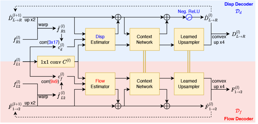
We adopt the flow decoder from ARFlow [48] due to its simplicity and light weight. As shown in the lower part of Fig. 2(b), our flow decoder contains a warping and correlation module, a flow estimator network, a context network, as well as a learned upsampler network suggested by SemARFlow [93]. The decoder is applied recurrently to refine flow estimate starting from zero flow until 1/4 resolution . The upsampled is then used as the final output of the flow decoder. We refer readers to the original papers [48, 93] for more details.
The disparity decoder structure is shown in the upper part of Fig. 2(b). We copy the same structure from the flow decoder except for the following small changes.
-
•
We change the window size of the pairwise correlation module from to to make the disparity decoder focus more along the horizontal direction.
-
•
We use a new disparity estimator to replace the flow estimator network since the number of input channels has changed as we change the correlation module.
-
•
We apply negative ReLU, which filters only negative values, before upsampling to make sure our left-to-right disparity output is negative.
-
•
We add a redundant -channel of all zeros to the estimated 1D disparity to make it 2D so that we can reuse the same context network and learned upsampler.
Loss
We apply the same photometric and augmentation loss as in [93] for both flow and disparity, which are then linearly combined with weights .
3.4 Stage 2: Pixel-Level Rigid Motion Estimation
Many previous methods have shown successful examples of reconstructing optical flow using depth maps and the 6-DoF rigid motion [33, 53, 83, 47, 10]. Nevertheless, most methods only estimate the rigid motion of the camera, assuming that the whole scene is stationary. This is problematic for dynamic objects such as moving vehicles.
Pixel-Level Rigid Motion Map
In contrast, we explore estimating rigid motion for every rigid body in the view to enhance flow reconstruction. Since the number of objects in each frame is variable, inspired by RAFT-3D [73], we represent rigid motion at the pixel-level as a dense map , where is the 3D Special Euclidean group for rigid motions [22]. The rigid motion of each pixel is defined as the rigid motion of the object to which that pixel belongs. This map not only contains full rigid motion information of the scene, but also implies a segmentation of rigid bodies.
Reconstructing Flow from Disparity and Rigid Motion
Suppose is a point from the reference frame , and its disparity has been estimated as . We can compute its depth and its 3D coordinates by
| (1) |
where is the camera intrinsics matrix, is the horizontal focal distance of the camera, and is the baseline distance between left and right cameras [15].
Suppose the point belongs to a rigid body that has rigid motion . The coordinates of that point in the next camera coordinates system will be , which can be projected back to the frame by
| (2) |
where is the corresponding position and is its new depth in the new frame. The reconstructed optical flow is then . Note that we only update the optical flow in Stage 2 with no refinement on disparities.
Network
We borrow RAFT-3D [73] as our network structure. RAFT-3D is a supervised scene flow network that takes RGBD inputs and estimates rigid motion maps using a Dense-SE3 layer [73]. The rigid motion maps are recurrently refined and used to reconstruct scene flow, which is then supervised by labels in an end-to-end manner.
Different from RAFT-3D, our system only takes RGB inputs without depths, as defined in Sec. 3.1. We also do not have the scene flow labels for supervision. Therefore, we use our Stage-1 model to generate depth inputs and flow pseudo-labels to train the model.
Since our Stage-1 outputs may not be reliable in occlusion regions, we also estimate their occlusion masks through forward-backward consistency check [55]. The occlusion regions for both disparities and flows are masked out in the loss, so we only penalize at places where both our predictions and pseudo-labels are reliable. More details are included in Appendix A.2.
Loss
RAFT-3D [73] is originally trained with a supervised scene flow loss, which can be computed using our pseudo-labels from Stage-1 model inference. In addition, we add a smoothness loss to better constrain our rigid motion map. Specifically, we compute the first-order gradient of the 6D rigid motion map and take its L1 norm as our smoothness loss, which is applied to estimates at all decoder iterations in accordance with the original RAFT-3D loss. We expect that the rigid motion for occlusion regions can be imputed based on local smoothness, which allows us to reconstruct occluded flow accurately.
| Methods | Joint? | Stereo? | KITTI-2012 | KITTI-2015 | |||||
| train | test | train | test | ||||||
| EPE | EPE | EPE-all | EPE-noc | EPE-occ | Fl-all | Fl-all | |||
| SelFlow [51] | 1.69 | 2.2 | 4.84 | - | - | - | 14.19 | ||
| ARFlow [48] | 1.44 | 1.8 | 2.85 | - | - | - | 11.80 | ||
| UPFlow [54] | 1.27 | 1.4 | 2.45 | - | - | - | 9.38 | ||
| DF-Net [99] | ✔ | 3.54 | 4.4 | 8.98 | - | - | 26.01 | 25.70 | |
| CC-uft [60] | ✔ | - | - | 5.66 | - | - | 20.93 | 25.27 | |
| EPC++ (mono) [53] | ✔ | 2.30 | 2.6 | 5.84 | - | - | - | 21.56 | |
| EPC++ (stereo) [53] | ✔ | ✔ | 1.91 | 2.2 | 5.43 | - | - | - | 20.52 |
| UnOS [83] | ✔ | ✔ | 1.92 | - | 5.58 | - | - | - | 18.00 |
| UnRigidFlow [47] | ✔ | ✔ | 1.64 | 1.8 | 5.19 | - | - | - | 11.66 |
| Flow2Stereo [50] | ✔ | ✔ | 1.45 | 1.7 | 3.54 | 2.12 | - | - | 11.10 |
| EffiScene [33] | ✔ | ✔ | 1.68 | - | 4.20 | - | - | 14.31 | 13.08 |
| FLC [10] | ✔ | ✔ | 1.25 | 1.5 | 2.35 | 1.57 | 6.68 | 9.09 | 9.70 |
| Ours (Stage 1) | ✔ | ✔ | 1.26 | 1.5 | 2.31 | 1.70 | 5.31 | 7.93 | 9.01 |
| Ours (Stage 2) | ✔ | ✔ | 1.04 | 1.2 | 2.04 | 1.49 | 4.78 | 6.87 | 7.63 |
| Ours (Stage 3) | ✔ | ✔ | 1.02 | 1.2 | 1.99 | 1.42 | 4.87 | 6.65 | 7.36 |
| Methods | Error (Lower is Better) | Accuracy (Higher is Better) | |||||
| Abs Rel | Sq Rel | RMSE | RMSE-log | ||||
| Godard et al. [19] | 0.068 | 0.835 | 4.392 | 0.146 | 0.942 | 0.978 | 0.989 |
| UnOS [83] | 0.049 | 0.515 | 3.404 | 0.121 | 0.965 | 0.984 | 0.992 |
| UnRigidFlow [47] | 0.051 | 0.532 | 3.780 | 0.126 | 0.957 | 0.982 | 0.991 |
| EffiScene [33] | 0.049 | 0.522 | 3.461 | 0.120 | 0.961 | 0.984 | 0.992 |
| FLC [10] | 0.047 | 0.394 | 3.358 | 0.119 | - | - | - |
| Ours (Stage 1 & Stage 2) | 0.048 | 0.574 | 3.616 | 0.118 | 0.970 | 0.986 | 0.992 |
| Ours (Stage 3) | 0.047 | 0.565 | 3.588 | 0.118 | 0.971 | 0.986 | 0.992 |
3.5 Stage 3: Fusion and Post-Processing
We now have two different optical flow estimates based on photometric (Stage 1) and geometric (Stage 2) constraints, so we find a way to fuse them. Also, our disparity is not refined in Stage 2, so we refine it here based on the dense rigid motion maps.
Flow Fusion
The previous stages estimate flow in two different ways, namely 2D photometric matching (Stage 1) and 3D motion reconstruction (Stage 2). These flows are reliable in different regions, so we fuse them in light of that.
We reuse the occlusion masks computed in Stage 2 to define reliable pixels for both flows. For Stage-1 flow , we define flow on non-occluded pixels as reliable. For Stage-2 flow, since it is reconstructed from the disparity map, we adopt the disparity occlusion mask and define its non-occluded pixels as reliable. Note that the flow occlusion regions are usually larger than disparity occlusions, unless the motion is very small. This indicates that our Stage-2 flow is generally more reliable than Stage 1 in typical scenarios.
To fuse the two flows, we examine their reliabilities at each pixel. If both flows are reliable, we take the average. If exactly one of them is reliable, we copy that reliable estimate. If none of them is reliable, we stick to Stage-2 flow due to its better overall performance.
Disparity Refinement
We aim to refine disparities given the rigid motion map and flow. For a pixel , its correspondence can be found using the fused flow above. Similar as shown in Eqs. 2 and 1, we can un-project the pixels to 3D camera coordinates and find their relationships from rigid motion as follows,
| (3) |
where are the disparities of the same point in . Our current estimates can be retrieved from Stage-1 model outputs (flow warping needed to compute ), and we optimize so that Eq. 3 holds. We can rewrite Eq. 3 as
| (4) |
where we denote constant vectors as
| (5) |
To linearize Eq. 4, we do first-order Taylor’s expansions for around zero and since , we get
| (6) |
which is an over-determined linear system in and can be solved in the least-squares sense in closed form [1].
4 Experiments

4.1 Datasets
We experiment on KITTI datasets [16, 56]. For all stages, our models are first trained on KITTI raw frames (25.2k samples) and then fine-tuned on KITTI multi-view extensions (6.7k samples), as suggested by ARFlow [48]. We validate our model using KITTI-2015 [56] and 2012 [16] training sets (around 200 samples for each).
4.2 Implementation Details
We train our Stage 1 and 2 PyTorch [58] models (see code in the supplementary material) with the Adam optimizer [38] with batch size 4. Stage 3 requires no training.
In Stage 1, we adopt the refined schedule from SemARFlow [93] and train on raw frames for 100k iterations with a fixed learning rate 2e-4 and then on the multi-view extension set for another 100k iterations with the OneCycleLR scheduler [69] (max learning rate 4e-4). In Stage 2, we apply the same scheduler but adjust the iterations as in RAFT-3D [73]. We first train on raw for 200k iterations and then on multi-view for 50k iterations. All other implementation details are the same as in the originals (ARFlow [48] for Stage 1 and RAFT-3D [73] for Stage 2).
We augment training data with appearance transformations (brightness, contrast, saturation, hue, gaussian blur, etc.) and randomly swap the input images both in time ( and ) and space ( and ). With spatial swaps we also flip the images horizontally to ensure negative disparity. The inputs are resized to in Stage 1 but cropped to in Stage 2 to save memory.
| Methods | Disparity 1 | Disparity 2 | Optical Flow | Scene Flow | ||||||||
|---|---|---|---|---|---|---|---|---|---|---|---|---|
| bg | fg | all | bg | fg | all | bg | fg | all | bg | fg | all | |
| UnOS [83] | 5.10 | 14.55 | 6.67 | 9.61 | 24.28 | 12.05 | 16.93 | 23.34 | 18.00 | 19.70 | 35.43 | 22.32 |
| Ours (Stage 1) | 3.65 | 15.04 | 5.55 | 14.59 | 20.09 | 15.50 | 7.91 | 14.52 | 9.01 | 18.13 | 28.26 | 19.82 |
| Ours (Stage 2) | 3.65 | 15.04 | 5.55 | 5.30 | 20.50 | 7.83 | 5.96 | 15.96 | 7.63 | 7.64 | 26.25 | 10.74 |
| Optical Flow Error | Depth Error | ||||||||
| EPE-all | EPE-noc | EPE-occ | Fl-all | Abs Rel | Sq Rel | RMSE | RMSE-log | ||
| 1 | 0 | 2.38 | 1.73 | 5.56 | 8.02 | - | - | - | - |
| 0.9 | 0.1 | 2.38 | 1.74 | 5.52 | 8.07 | 0.049 | 0.618 | 3.692 | 0.120 |
| 0.7* | 0.3* | 2.31 | 1.71 | 5.31 | 7.93 | 0.048 | 0.574 | 3.616 | 0.118 |
| 0.5 | 0.5 | 2.34 | 1.73 | 5.30 | 7.94 | 0.048 | 0.593 | 3.628 | 0.118 |
| 0.3 | 0.7 | 2.38 | 1.77 | 5.32 | 8.10 | 0.050 | 0.695 | 3.672 | 0.119 |
| 0.1 | 0.9 | 36.92 | 27.95 | 73.69 | 83.96 | 0.050 | 0.596 | 3.658 | 0.120 |
| 0 | 1 | - | - | - | - | 0.050 | 0.586 | 3.646 | 0.120 |
| Shared? | Disp. corr. | Optical Flow Error | Depth Error | ||||||||
|---|---|---|---|---|---|---|---|---|---|---|---|
| Flow | Context | Up | EPE-all | EPE-noc | EPE-occ | Fl-all | Abs Rel | Sq Rel | RMSE | RMSE-log | |
| ✔ | ✔ | ✔ | 2.37 | 1.71 | 5.51 | 8.06 | 0.051 | 0.754 | 3.785 | 0.122 | |
| ✔ | ✔ | 2.34 | 1.71 | 5.32 | 7.96 | 0.048 | 0.588 | 3.613 | 0.118 | ||
| ✔* | ✔* | * | 2.31 | 1.70 | 5.31 | 7.93 | 0.048 | 0.574 | 3.616 | 0.118 | |
| ✔ | 2.34 | 1.71 | 5.32 | 8.03 | 0.048 | 0.593 | 3.625 | 0.118 | |||
| 2.36 | 1.72 | 5.39 | 8.02 | 0.047 | 0.555 | 3.565 | 0.117 | ||||
| Options | Train | Test | ||||
|---|---|---|---|---|---|---|
| Mask | Smooth | Fl-all | Fl-all | Fl-noc | Fl-bg | Fl-fg |
| 8.47 | 9.53 | 6.93 | 8.38 | 15.25 | ||
| ✔ | 7.19 | 7.87 | 6.42 | 6.56 | 14.42 | |
| ✔* | ✔* | 6.87 | 7.63 | 6.29 | 5.96 | 15.96 |

4.3 Benchmark Test Results
Optical Flow
As shown in Tab. 1, even our Stage 1 results outperform all previous state-of-the-art unsupervised methods including FLC[10] and UPFlow [54] on all metrics on KITTI-2015 [56] and 2012 [16]. Through rigid motion estimation in Stage 2, our reconstructed flow results improve even further. After leveraging and fusing flows in the first two stages, our Stage 3 finally achieves the best test errors (7.36%) on KITTI-2015, a 20%+ decrease compared with the state-of-the-art UPFlow [54] (9.38%). These results strongly indicate that all our stages contribute significantly to improving flow results.
Stereo Depth
Since we do not refine disparity in Stage 2, disparities from Stage 1 and 2 are the same. Tab. 2 shows that our Stage 1 and 2 results outperform the state of the art on most evaluation metrics (still comparable if not better). The Stage-3 refinement also improves the squared relative error and RMSE, indicating better depths on far-away objects. Stereo matching is known to be an easier problem than optical flow, so it has less margin for improvement.
4.4 Qualitative Examples
The examples in Fig. 3 illustrate how each stage works compared with UPFlow [54] (state-of-the-art) and ARFlow [48] (the backbone of our Stage-1 model).
Our Stage-1 results are visually comparable with the state-of-the-art methods. After applying pixel-level rigid motion estimation in Stage 2, our method handles occlusions around moving cars better, whether they are in the foreground (Row 1 and 3) or occluded by other objects like poles (Row 2). This is consistent with our claim that the occluded flow can be reconstructed based on stereo depth, which is generally more reliable.
Rows 3 and 4 in Fig. 3 show that our Stage-3 refinement can help sharpen thin foreground objects like traffic lights and poles. In this example, the traffic light is moving to the right. The Stage-1 flow is only sharp on the left side due to occlusions on the right, whereas the Stage-2 flow is only sharp on the right due to disparity occlusions on the left. By analyzing the reliable regions of each output, our fused Stage-3 output is sharp on both sides of the object. This illustrates a typical way in which Stage 3 improves, i.e. by combining the flow results from photometric (Stage 1) and geometric (Stage 2) constraints that are usually reliable in different regions.
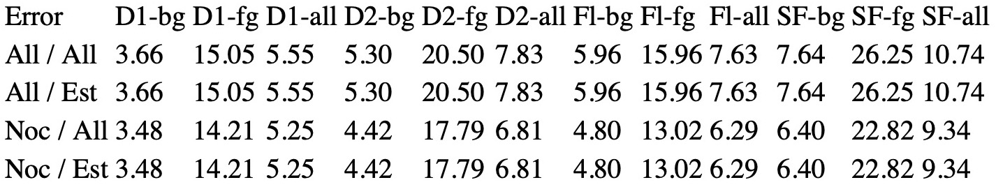
4.5 Scene Flow Evaluations
As in RAFT-3D [73], we evaluate our Stage-2 rigid motion estimates via scene flow due to lack of dense rigid-motion ground truth. Our Stage 1 does not output “Disparity 2” (the changed disparity of points from the first frame), so we approximate it by warping our first-pair disparity with flow. Tab. 3 shows that our Stage-2 rigid motion estimation very much improves scene flow results, suggesting that it captures dense 3D rigid motions well.
4.6 Ablation Studies
Balancing Optical Flow and Disparity in Stage 1
Tab. 4 shows that are the best balancing weights for flow and disparity losses in Stage 1. We also compare with settings where we train on either flow or disparity alone using the same network and show that our joint network benefits both tasks.
Different Options of Shared Decoders in Stage 1
We examine different options for how the two decoders in Stage 1 share model weights, from the most shared (Row 1) to the least shared setting (Row 5). Tab. 5 shows that our final setting has the best flow results while maintaining comparable depth evaluations.
Changes to RAFT-3D in Stage 2
Tab. 6 shows that our proposed changes in Stage 2 are necessary to optimize RAFT-3D [73] in the unsupervised setting. Moreover, Fig. 4 visualizes the 6 DoF rigid motion field in RGB colors after reducing dimensionality to 3 with PCA [59]. The added smoothness loss clearly helps separate all rigid bodies in the frame. This also implies that our dense rigid motion map can potentially be used to generate rigid body segmentation masks, which we discuss in Appendix B.3.
4.7 Time Efficiency
We time our stages and show that they run efficiently. We infer input samples of dimension on one NVIDIA GeForce RTX 2080 Ti GPU. Our Stage-1 model contains 3.2 million parameters and can infer both flow and disparity together in seconds. Our Stage-2 model contains 6.0 million parameters and can perform dense rigid motion estimation and flow reconstruction in seconds. Our Stage 3 is a simple post-processing stage and runs instantly on CPUs.
5 Conclusion
We propose UFD-PRiME, a system for the joint unsupervised training of optical flow and stereo depth using pixel-level rigid motion estimation. We first design a simple yet effective unsupervised network based on ARFlow [48] to train flow and disparity jointly, where we use separate decoders with partial weight-sharing modules to handle the two tasks. Then, we train a pixel-level rigid motion estimation network adapted from RAFT-3D [73] to estimate dense 3D rigid motion maps, which are then used to reconstruct flow once again given depth. Finally, we fuse and refine flow and disparities by reliability analysis and stereo geometry. Our method outperforms all previous methods significantly on optical flow errors on the KITTI benchmarks [16, 56], especially on occlusion regions and around dynamic objects, while maintaining marginally better stereo depth evaluations.
Limitations
Estimating rigid motion for each pixel alone can be sensitive. For each 2D motion vector observed in the image plane, there are many different 3D rigid motions that can generate the same 2D projected motion. In our system, we use a smoothness loss on the rigid motion map to alleviate this issue. A possibly better solution is to aggregate object and instance level information so that we can assign the same rigid motion to every pixel on the same rigid body. We leave this study for future work.
Appendix
Appendix A Method Details
A.1 Stage 1
Detailed Structures
The detailed network structure of our encoder, flow decoder, and disparity decoder are shown in Figs. 5(a), 5(b) and 5(c). The dimension of each intermediate tensor and the number of parameters are noted in the figures.


Redundant Dimension in Disparity
To reuse modules across flow and disparity decoders, we need to make sure their input sizes to the same module are equal. Therefore, in our implementation, our disparity is estimated as a 2D vector. In the disparity estimator module, which is not shared, the output dimension is set as 1, so we only change the -dimension of the disparity estimate. For other shared modules, we use 2D disparities as both input and output. In the end, we drop the -dimension of our 2D disparity estimate to make sure our final disparity is strictly 1D.
Augmentation as Self-Supervision
Our network is adapted from ARFlow [48], which has an “augmentation as self-supervision” module. In ARFlow, after each forward pass of the current sample, they apply some random transformations, including appearance transformations (brightness, contrast, hue, saturation, gaussian blur, etc.), spatial transformations (random affine), and occlusion transformations (random cropping), to generate an augmented sample as well as its pseudo-label. Then, they do a second forward pass using the augmented sample and self-supervise the output using the generated pseudo-label. This self-supervision module helps learn flow at occlusion regions and enhance the consistency of optical flow prediction.
We keep their augmentation as self-supervision module in training, and we apply the same transformations to all three input images, , at the same time to simulate a realistic transformation to the moving stereo camera rig. However, we have to turn off the random rotation part in the random affine transformation to ensure the left and right views are on the same horizontal line. We assume 1D horizontal search for disparities, and if rotations are applied, the true disparity will no longer be 1D, which affects the effectiveness of our disparity decoder.
A.2 Stage 2
Computing Occlusion Masks
We first use the Stage-1 model to generate all the flow and disparities needed for Stage-2 training. In addition to the regular outputs shown in the Stage-1 network, we also compute all other flows and disparities (including backward ones) among the four input images , as enumerated in Fig. 6. This can be done by switching different inputs to the Stage-1 network. For example, we can compute by feeding to the network. Note that if we swap the left and right view, we also need to do a horizontal flip to all input images to ensure the disparity is negative. We can then horizontally flip the disparity output again to recover the original disparity.

With all flows and disparities estimated, we compute all occlusion masks through forward-backward consistency check [55] as follows. Suppose and are the forward and backward pair of flows (or disparities) and is a point in the frame. We flag the forward occlusion mask as 1 on whenever the following constraint holds.
where we use hyper-parameters , as in [55]. We compute occlusion masks for every forward and backward flow and disparities computed and store them on the disk for later use.
Generating Scene Flow Pseudo-labels for RAFT-3D
The RAFT-3D [73] network also requires a disparity channel input to become RGBD inputs. We can simply use the disparities estimated by the Stage-1 model for that.
In loss computation, RAFT-3D requires scene flow pseudo-labels, which include the regular 2D optical flow, as well as a disparity change value to indicate the motion on the depth dimension. For the former, we can simply use the previous flow estimate. For the latter, we need to warp previous disparities. For example, to compute scene flow pseudo-label between and , for each point , we warp and compute the disparity change pseudo-label as follows.
We mask out the unreliable regions of both scene flow estimates and pseudo-labels when we compute loss. Since our flow in Stage 2 is reconstructed from disparity , the unreliable region of the flow estimate is simply the estimated occlusion region of . The unreliable region of pseudo-label is generated as a union of the occlusion regions of , , and the warped .
A Smaller Context Network
Our Stage-2 network is exactly the same as RAFT-3D [73] except for one change on the context network. The original RAFT-3D uses a very large context network copied from FPN [45] so that they can use semantically pre-trained weights to help better distinguish objects. In our experiment, we found empirically that using a much smaller context network such as the same structure of the feature encoder network still gives similar results. Therefore, we stick to the smaller context network to save memory.
A.3 Stage 3
Depth Refinement
Continuing the derivation in the main paper, we need to solve the following over-determined linear system
which can be rewritten as
Denoting , , , we then have
This over-determined linear system can be approximately solved based on least squared error criterion as
where .
We linearize this equation here instead of solving it in the depth domain (which could be more straightforward) because solving this type of linear systems could be very sensitive in the depth domain. For example, when the 3D motion is along the moving direction of the camera, we have the projection rays from the two consecutive frames almost in parallel, so the matrix here will be close to rank 1. To avoid this issue, we discard the refinement if is close to singular (decided by the opencv package automatically).
Appendix B Experiment Details
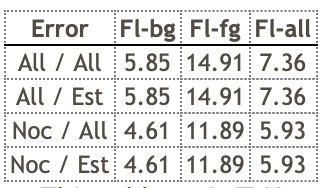
B.1 Screenshots of Benchmark Results
We show the benchmark test screenshots for all our three stages from the KITTI [56] website in Figs. 7, 8 and 9 to prove that our results are official. Our final-stage result entry (currently anonymous) is also shown on the official website now for your reference.

B.2 More Qualitative Examples

B.3 Visualizing Rigid Motions Segmentation
Our rigid motion also implies a soft segmentation of rigid bodies that we can refer to. This can be computed using traditional clustering algorithms based on our 6-DoF map. However, the selection of clustering method also makes a difference here. It may also be helpful if we could have object-level information to regularize our map segmentation. Thus, we leave this for future research.
Alternatively, we can also visualize the map in RGB through PCA. For cases with exactly 3 distinct rigid motions, we can see the segmentation very clearly after normalizing the first three principal component channel-wise to between 0 and 1, as shown in the last figure in the main paper. For most cases that do not have at least three distinct rigid motions, normalizing the top 3 principal components channel-wise may magnify the small changes represented by the second or third color channel. In that case, we suggest normalizing all three channels together. One example of that is shown in our Fig. 1 in the main paper.
References
- [1] Howard Anton and Chris Rorres. Elementary linear algebra: applications version. John Wiley & Sons, 2013.
- [2] Connelly Barnes, Eli Shechtman, Adam Finkelstein, and Dan B Goldman. Patchmatch: A randomized correspondence algorithm for structural image editing. ACM TOG, 28(3):24, 2009.
- [3] Ejder Bastug, Mehdi Bennis, Muriel Médard, and Mérouane Debbah. Toward interconnected virtual reality: Opportunities, challenges, and enablers. IEEE Communications Magazine, 55(6):110–117, 2017.
- [4] Bayram Bayramli, Junhwa Hur, and Hongtao Lu. Raft-msf: Self-supervised monocular scene flow using recurrent optimizer. IJCV, pages 1–13, 2023.
- [5] Paul J Besl and Neil D McKay. Method for registration of 3-d shapes. In Sensor Fusion IV: Control Paradigms and Data Structures, volume 1611, pages 586–606. Spie, 1992.
- [6] Nicolas Carion, Francisco Massa, Gabriel Synnaeve, Nicolas Usunier, Alexander Kirillov, and Sergey Zagoruyko. End-to-end object detection with transformers. In ECCV, pages 213–229. Springer, 2020.
- [7] Jia-Ren Chang and Yong-Sheng Chen. Pyramid stereo matching network. In CVPR, pages 5410–5418, 2018.
- [8] Guanying Chen, Kai Han, Boxin Shi, Yasuyuki Matsushita, and Kwan-Yee K Wong. Deep photometric stereo for non-lambertian surfaces. IEEE TPAMI, 44(1):129–142, 2020.
- [9] Xinjing Cheng, Peng Wang, and Ruigang Yang. Learning depth with convolutional spatial propagation network. IEEE TPAMI, 42(10):2361–2379, 2019.
- [10] Cheng Chi, Qingjie Wang, Tianyu Hao, Peng Guo, and Xin Yang. Feature-level collaboration: Joint unsupervised learning of optical flow, stereo depth and camera motion. In CVPR, pages 2463–2473, 2021.
- [11] Xingshuai Dong, Matthew A Garratt, Sreenatha G Anavatti, and Hussein A Abbass. Towards real-time monocular depth estimation for robotics: A survey. IEEE Trans. Intell. Transport. Sys., 23(10):16940–16961, 2022.
- [12] Alexey Dosovitskiy, Lucas Beyer, Alexander Kolesnikov, Dirk Weissenborn, Xiaohua Zhai, Thomas Unterthiner, Mostafa Dehghani, Matthias Minderer, Georg Heigold, Sylvain Gelly, Jakob Uszkoreit, and Neil Houlsby. An image is worth 16x16 words: Transformers for image recognition at scale. In ICLR, 2021.
- [13] Alexey Dosovitskiy, Philipp Fischer, Eddy Ilg, Philip Hausser, Caner Hazirbas, Vladimir Golkov, Patrick Van Der Smagt, Daniel Cremers, and Thomas Brox. Flownet: Learning optical flow with convolutional networks. In ICCV, pages 2758–2766, 2015.
- [14] Martin A Fischler and Robert C Bolles. Random sample consensus: a paradigm for model fitting with applications to image analysis and automated cartography. ACM Communications, 24(6):381–395, 1981.
- [15] David A Forsyth and Jean Ponce. Computer vision: a modern approach. prentice hall professional technical reference, 2002.
- [16] Andreas Geiger, Philip Lenz, Christoph Stiller, and Raquel Urtasun. Vision meets robotics: The kitti dataset. IJRR, 32(11):1231–1237, 2013.
- [17] Andreas Geiger, Philip Lenz, and Raquel Urtasun. Are we ready for autonomous driving? the kitti vision benchmark suite. In CVPR, pages 3354–3361. IEEE, 2012.
- [18] Ross Girshick. Fast r-cnn. In ICCV, pages 1440–1448, 2015.
- [19] Clément Godard, Oisin Mac Aodha, and Gabriel J Brostow. Unsupervised monocular depth estimation with left-right consistency. In CVPR, pages 270–279, 2017.
- [20] Xiaoyang Guo, Kai Yang, Wukui Yang, Xiaogang Wang, and Hongsheng Li. Group-wise correlation stereo network. In CVPR, pages 3273–3282, 2019.
- [21] Marsha Jo Hannah. Computer matching of areas in stereo images. Stanford University, 1974.
- [22] Richard Hartley and Andrew Zisserman. Multiple view geometry in computer vision. Cambridge university press, 2003.
- [23] Kaiming He, Xiangyu Zhang, Shaoqing Ren, and Jian Sun. Identity mappings in deep residual networks. In ECCV, pages 630–645. Springer, 2016.
- [24] Heiko Hirschmuller. Stereo processing by semiglobal matching and mutual information. IEEE TPAMI, 30(2):328–341, 2007.
- [25] Jonathan Ho, Ajay Jain, and Pieter Abbeel. Denoising diffusion probabilistic models. NeurIPS, 33:6840–6851, 2020.
- [26] Berthold KP Horn and Brian G Schunck. Determining optical flow. Artificial Intelligence, 17(1-3):185–203, 1981.
- [27] Hsin-Ping Huang, Charles Herrmann, Junhwa Hur, Erika Lu, Kyle Sargent, Austin Stone, Ming-Hsuan Yang, and Deqing Sun. Self-supervised autoflow. In CVPR, pages 11412–11421, 2023.
- [28] Zhaoyang Huang, Xiaoyu Shi, Chao Zhang, Qiang Wang, Ka Chun Cheung, Hongwei Qin, Jifeng Dai, and Hongsheng Li. Flowformer: A transformer architecture for optical flow. In ECCV, pages 668–685. Springer, 2022.
- [29] Junhwa Hur and Stefan Roth. Iterative residual refinement for joint optical flow and occlusion estimation. In CVPR, pages 5754–5763, 2019.
- [30] Junhwa Hur and Stefan Roth. Self-supervised monocular scene flow estimation. In CVPR, pages 7396–7405, 2020.
- [31] Joel Janai, Fatma Guney, Anurag Ranjan, Michael Black, and Andreas Geiger. Unsupervised learning of multi-frame optical flow with occlusions. In ECCV, pages 690–706, 2018.
- [32] Shihao Jiang, Dylan Campbell, Yao Lu, Hongdong Li, and Richard Hartley. Learning to estimate hidden motions with global motion aggregation. In ICCV, pages 9772–9781, 2021.
- [33] Yang Jiao, Trac D Tran, and Guangming Shi. Effiscene: Efficient per-pixel rigidity inference for unsupervised joint learning of optical flow, depth, camera pose and motion segmentation. In CVPR, pages 5538–5547, 2021.
- [34] Sunghun Joung, Seungryong Kim, Kihong Park, and Kwanghoon Sohn. Unsupervised stereo matching using confidential correspondence consistency. IEEE Trans. Intell. Transport. Sys., 21(5):2190–2203, 2019.
- [35] Hyunyoung Jung, Zhuo Hui, Lei Luo, Haitao Yang, Feng Liu, Sungjoo Yoo, Rakesh Ranjan, and Denis Demandolx. Anyflow: Arbitrary scale optical flow with implicit neural representation. In CVPR, pages 5455–5465, 2023.
- [36] Alex Kendall, Hayk Martirosyan, Saumitro Dasgupta, Peter Henry, Ryan Kennedy, Abraham Bachrach, and Adam Bry. End-to-end learning of geometry and context for deep stereo regression. In ICCV, pages 66–75, 2017.
- [37] Hannah Halin Kim, Shuzhi Yu, Shuai Yuan, and Carlo Tomasi. Cross-attention transformer for video interpolation. In ACCVW, pages 320–337, 2022.
- [38] Diederik P Kingma and Jimmy Ba. Adam: A method for stochastic optimization. ICLR, 2014.
- [39] Vladimir Kolmogorov. Convergent tree-reweighted message passing for energy minimization. In International Workshop on Artificial Intelligence and Statistics, pages 182–189. PMLR, 2005.
- [40] Fanjie Kong, Shuai Yuan, Weituo Hao, and Ricardo Henao. Mitigating test-time bias for fair image retrieval. In NeurIPS, 2023.
- [41] Alex Krizhevsky, Ilya Sutskever, and Geoffrey E Hinton. Imagenet classification with deep convolutional neural networks. NeurIPS, 25, 2012.
- [42] Hsueh-Ying Lai, Yi-Hsuan Tsai, and Wei-Chen Chiu. Bridging stereo matching and optical flow via spatiotemporal correspondence. In CVPR, pages 1890–1899, 2019.
- [43] Vincent Lepetit, Francesc Moreno-Noguer, and Pascal Fua. Epnp: An accurate o(n) solution to the pnp problem. IJCV, 81:155–166, 2009.
- [44] Ang Li, Zejian Yuan, Yonggen Ling, Wanchao Chi, Shenghao Zhang, and Chong Zhang. Unsupervised occlusion-aware stereo matching with directed disparity smoothing. IEEE Trans. Intell. Transport. Sys., 23(7):7457–7468, 2021.
- [45] Tsung-Yi Lin, Piotr Dollár, Ross Girshick, Kaiming He, Bharath Hariharan, and Serge Belongie. Feature pyramid networks for object detection. In CVPR, pages 2117–2125, 2017.
- [46] Lahav Lipson, Zachary Teed, and Jia Deng. Raft-stereo: Multilevel recurrent field transforms for stereo matching. In 3DV, pages 218–227. IEEE, 2021.
- [47] Liang Liu, Guangyao Zhai, Wenlong Ye, and Yong Liu. Unsupervised learning of scene flow estimation fusing with local rigidity. In IJCAI, pages 876–882, 2019.
- [48] Liang Liu, Jiangning Zhang, Ruifei He, Yong Liu, Yabiao Wang, Ying Tai, Donghao Luo, Chengjie Wang, Jilin Li, and Feiyue Huang. Learning by analogy: Reliable supervision from transformations for unsupervised optical flow estimation. In CVPR, pages 6489–6498, 2020.
- [49] Pengpeng Liu, Irwin King, Michael R Lyu, and Jia Xu. Ddflow: Learning optical flow with unlabeled data distillation. In AAAI, volume 33, pages 8770–8777, 2019.
- [50] Pengpeng Liu, Irwin King, Michael R Lyu, and Jia Xu. Flow2stereo: Effective self-supervised learning of optical flow and stereo matching. In CVPR, pages 6648–6657, 2020.
- [51] Pengpeng Liu, Michael Lyu, Irwin King, and Jia Xu. Selflow: Self-supervised learning of optical flow. In CVPR, pages 4571–4580, 2019.
- [52] Bruce D Lucas and Takeo Kanade. An iterative image registration technique with an application to stereo vision. In IJCAI, volume 2, pages 674–679, 1981.
- [53] Chenxu Luo, Zhenheng Yang, Peng Wang, Yang Wang, Wei Xu, Ram Nevatia, and Alan Yuille. Every pixel counts++: Joint learning of geometry and motion with 3d holistic understanding. IEEE TPAMI, 42(10):2624–2641, 2019.
- [54] Kunming Luo, Chuan Wang, Shuaicheng Liu, Haoqiang Fan, Jue Wang, and Jian Sun. Upflow: Upsampling pyramid for unsupervised optical flow learning. In CVPR, pages 1045–1054, 2021.
- [55] Simon Meister, Junhwa Hur, and Stefan Roth. Unflow: Unsupervised learning of optical flow with a bidirectional census loss. In AAAI, volume 32, 2018.
- [56] Moritz Menze and Andreas Geiger. Object scene flow for autonomous vehicles. In CVPR, 2015.
- [57] Mahmoud A Mohamed, Hatem A Rashwan, Bärbel Mertsching, Miguel Angel García, and Domenec Puig. Illumination-robust optical flow using a local directional pattern. IEEE TCSVT, 24(9):1499–1508, 2014.
- [58] Adam Paszke, Sam Gross, Francisco Massa, Adam Lerer, James Bradbury, Gregory Chanan, Trevor Killeen, Zeming Lin, Natalia Gimelshein, Luca Antiga, Alban Desmaison, Andreas Kopf, Edward Yang, Zachary DeVito, Martin Raison, Alykhan Tejani, Sasank Chilamkurthy, Benoit Steiner, Lu Fang, Junjie Bai, and Soumith Chintala. Pytorch: An imperative style, high-performance deep learning library. In NeurIPS, pages 8024–8035. Curran Associates, Inc., 2019.
- [59] Karl Pearson. Liii. on lines and planes of closest fit to systems of points in space. The London, Edinburgh, and Dublin Philosophical Magazine and Journal of Science, 2(11):559–572, 1901.
- [60] Anurag Ranjan, Varun Jampani, Lukas Balles, Kihwan Kim, Deqing Sun, Jonas Wulff, and Michael J Black. Competitive collaboration: Joint unsupervised learning of depth, camera motion, optical flow and motion segmentation. In CVPR, pages 12240–12249, 2019.
- [61] Zhe Ren, Junchi Yan, Bingbing Ni, Bin Liu, Xiaokang Yang, and Hongyuan Zha. Unsupervised deep learning for optical flow estimation. In AAAI, 2017.
- [62] Zhile Ren, Orazio Gallo, Deqing Sun, Ming-Hsuan Yang, Erik B Sudderth, and Jan Kautz. A fusion approach for multi-frame optical flow estimation. In WACV, pages 2077–2086. IEEE, 2019.
- [63] Jerome Revaud, Philippe Weinzaepfel, Zaid Harchaoui, and Cordelia Schmid. Epicflow: Edge-preserving interpolation of correspondences for optical flow. In CVPR, pages 1164–1172, 2015.
- [64] Sebastian Ruder. An overview of multi-task learning in deep neural networks. arXiv preprint arXiv:1706.05098, 2017.
- [65] Sawhney. 3d geometry from planar parallax. In CVPR, pages 929–934. IEEE, 1994.
- [66] Johannes L Schonberger and Jan-Michael Frahm. Structure-from-motion revisited. In CVPR, pages 4104–4113, 2016.
- [67] Jianbo Shi et al. Good features to track. In CVPR, pages 593–600. IEEE, 1994.
- [68] Xiaoyu Shi, Zhaoyang Huang, Dasong Li, Manyuan Zhang, Ka Chun Cheung, Simon See, Hongwei Qin, Jifeng Dai, and Hongsheng Li. Flowformer++: Masked cost volume autoencoding for pretraining optical flow estimation. In CVPR, pages 1599–1610, 2023.
- [69] Leslie N Smith and Nicholay Topin. Super-convergence: Very fast training of neural networks using large learning rates. In Artificial Intelligence and Machine Learning for Multi-Domain Operations Applications, volume 11006, pages 369–386. SPIE, 2019.
- [70] Austin Stone, Daniel Maurer, Alper Ayvaci, Anelia Angelova, and Rico Jonschkowski. Smurf: Self-teaching multi-frame unsupervised raft with full-image warping. In CVPR, pages 3887–3896, 2021.
- [71] Deqing Sun, Xiaodong Yang, Ming-Yu Liu, and Jan Kautz. Pwc-net: Cnns for optical flow using pyramid, warping, and cost volume. In CVPR, pages 8934–8943, 2018.
- [72] Zachary Teed and Jia Deng. Raft: Recurrent all-pairs field transforms for optical flow. In ECCV, pages 402–419. Springer, 2020.
- [73] Zachary Teed and Jia Deng. Raft-3d: Scene flow using rigid-motion embeddings. In CVPR, pages 8375–8384, 2021.
- [74] Zachary Teed and Jia Deng. Tangent space backpropagation for 3d transformation groups. In Proceedings of the IEEE/CVF Conference on Computer Vision and Pattern Recognition (CVPR), 2021.
- [75] William P HG Thurston. Three-Dimensional Geometry and Topology, Volume 1: Volume 1. Princeton university press, 1997.
- [76] Philip HS Torr. Geometric motion segmentation and model selection. Philosophical Transactions of the Royal Society of London. Series A: Mathematical, Physical and Engineering Sciences, 356(1740):1321–1340, 1998.
- [77] Philip HS Torr, Andrew W Fitzgibbon, and Andrew Zisserman. The problem of degeneracy in structure and motion recovery from uncalibrated image sequences. IJCV, 32:27–44, 1999.
- [78] Shimon Ullman. The interpretation of structure from motion. Proceedings of the Royal Society of London. Series B. Biological Sciences, 203(1153):405–426, 1979.
- [79] René Vidal, Yi Ma, Stefano Soatto, and Shankar Sastry. Two-view multibody structure from motion. IJCV, 68(1):7–25, 2006.
- [80] René Vidal and Shankar Sastry. Optimal segmentation of dynamic scenes from two perspective views. In CVPR, volume 2, pages II–II. IEEE, 2003.
- [81] Sudheendra Vijayanarasimhan, Susanna Ricco, Cordelia Schmid, Rahul Sukthankar, and Katerina Fragkiadaki. Sfm-net: Learning of structure and motion from video. arXiv preprint arXiv:1704.07804, 2017.
- [82] Guangming Wang, Chi Zhang, Hesheng Wang, Jingchuan Wang, Yong Wang, and Xinlei Wang. Unsupervised learning of depth, optical flow and pose with occlusion from 3d geometry. IEEE Trans. Intell. Transport. Sys., 23(1):308–320, 2020.
- [83] Yang Wang, Peng Wang, Zhenheng Yang, Chenxu Luo, Yi Yang, and Wei Xu. Unos: Unified unsupervised optical-flow and stereo-depth estimation by watching videos. In CVPR, pages 8071–8081, 2019.
- [84] Yang Wang, Yi Yang, Zhenheng Yang, Liang Zhao, Peng Wang, and Wei Xu. Occlusion aware unsupervised learning of optical flow. In CVPR, pages 4884–4893, 2018.
- [85] Haofei Xu, Jing Zhang, Jianfei Cai, Hamid Rezatofighi, Fisher Yu, Dacheng Tao, and Andreas Geiger. Unifying flow, stereo and depth estimation. IEEE TPAMI, 2023.
- [86] Xun Xu, Loong-Fah Cheong, and Zhuwen Li. 3d rigid motion segmentation with mixed and unknown number of models. IEEE TPAMI, 43(1):1–16, 2019.
- [87] Gengshan Yang and Deva Ramanan. Learning to segment rigid motions from two frames. In CVPR, pages 1266–1275, 2021.
- [88] Zhichao Yin and Jianping Shi. Geonet: Unsupervised learning of dense depth, optical flow and camera pose. In CVPR, pages 1983–1992, 2018.
- [89] Jason J. Yu, Adam W. Harley, and Konstantinos G. Derpanis. Back to basics: Unsupervised learning of optical flow via brightness constancy and motion smoothness. In Gang Hua and Hervé Jégou, editors, ECCVW, pages 3–10, Cham, 2016. Springer International Publishing.
- [90] Shuzhi Yu, Hannah H Kim, Shuai Yuan, and Carlo Tomasi. Unsupervised flow refinement near motion boundaries. In BMVC. BMVA Press, 2022.
- [91] Chang Yuan, Gerard Medioni, Jinman Kang, and Isaac Cohen. Detecting motion regions in the presence of a strong parallax from a moving camera by multiview geometric constraints. IEEE TPAMI, 29(9):1627–1641, 2007.
- [92] Shuai Yuan, Xian Sun, Hannah Kim, Shuzhi Yu, and Carlo Tomasi. Optical flow training under limited label budget via active learning. In ECCV, pages 410–427, 2022.
- [93] Shuai Yuan, Shuzhi Yu, Hannah Kim, and Carlo Tomasi. Semarflow: Injecting semantics into unsupervised optical flow estimation for autonomous driving. In ICCV, pages 9566–9577, October 2023.
- [94] Ramin Zabih and John Woodfill. Non-parametric local transforms for computing visual correspondence. In ECCV, pages 151–158. Springer, 1994.
- [95] Feihu Zhang, Victor Prisacariu, Ruigang Yang, and Philip HS Torr. Ga-net: Guided aggregation net for end-to-end stereo matching. In CVPR, pages 185–194, 2019.
- [96] Feihu Zhang, Oliver J Woodford, Victor Adrian Prisacariu, and Philip HS Torr. Separable flow: Learning motion cost volumes for optical flow estimation. In ICCV, pages 10807–10817, 2021.
- [97] Chao Zhou, Hong Zhang, Xiaoyong Shen, and Jiaya Jia. Unsupervised learning of stereo matching. In ICCV, pages 1567–1575, 2017.
- [98] Tinghui Zhou, Matthew Brown, Noah Snavely, and David G Lowe. Unsupervised learning of depth and ego-motion from video. In CVPR, pages 1851–1858, 2017.
- [99] Yuliang Zou, Zelun Luo, and Jia-Bin Huang. Df-net: Unsupervised joint learning of depth and flow using cross-task consistency. In ECCV, pages 36–53, 2018.