Type-II Dirac photonic lattices
Abstract
Different from the Fermi surface of the type-I Dirac semimetal being a point, that of the type-II Dirac semimetal is a pair of crossing lines because the Dirac cone is tilted with open and hyperbolic isofrequency contours. As an optical analogy, type-II Dirac photonic lattices have been also designed. Here, we report type-II Dirac cones in Lieb-like photonic lattices composed of identical waveguide channels, and the anisotropy of the band structure is due to neither the refractive index change nor the environment, but only the spatial symmetry of the lattice; therefore, the proposal is advantage and benefits experimental observation. Conical diffractions and Klein tunneling in the parametric type-II photonic lattice are investigated in detail. Our results provide a simple and experimental feasible platform to study two-dimensional topological photonic and other nonrelativistic phenomena around type-II Dirac cones.
I Introduction
If a photonic lattice possesses Dirac cones Leykam and Desyatnikov (2016) in its band structure, it can be called a Dirac photonic lattice. One of the most famous Dirac photonic lattices is the photonic graphene Zandbergen and de Dood (2010); Rechtsman et al. (2013a, b); Crespi et al. (2013); Zeuner et al. (2014); Plotnik et al. (2014); Song et al. (2015); Nalitov et al. (2015), which is also known as the honeycomb lattice. In addition, the Lieb lattice Taie et al. (2015); Vicencio et al. (2015); Mukherjee et al. (2015); Diebel et al. (2016); Ozawa et al. (2017); Xia et al. (2018), the kagome lattice El Hassan et al. (2019); Li et al. (2019a), the superhoneycomb lattices Zhong et al. (2017); Kang et al. (2019), and some others Zhong et al. (2019) can be also classified into Dirac photonic lattices. It is worth mentioning that the Dirac cones of these photonic lattices aforementioned are mostly type-I, even though some of them are tilted. Actually, there are also type-II and type-III Dirac cones Milićević et al. (2019). The main difference between them is that the Fermi surface of the type-I Dirac cone is a point, that of the type-II Dirac cone is a pair of crossing lines, and that of the type-III Dirac cone is a line. In other words, the isofrequency contours of the type-I Dirac cones are closed, while those of the type-II counterparts are open and have hyperbolic profiles (e.g., on both and directions). The isofrequency contours of the type-III ones are also open, but only have hyperbolic profiles on one side (e.g., on either or direction). Note that there is also a different definition on the type-III degeneracy Li et al. (2019b). As a plethora of efforts being implemented to explore the type-II Weyl-like features Soluyanov et al. (2015); Xu et al. (2015); Chen et al. (2016); Autès et al. (2016); Noh et al. (2017a); Chen et al. (2018); Xie et al. (2019) both in condensed matter physics and photonics, type-II Dirac objects attract ongoing attentions too Yan et al. (2017); Noh et al. (2017b); Chang et al. (2017); Fei et al. (2018); Politano et al. (2018); Kim et al. (2018); Wang et al. (2018), especially in photonics Lin et al. (2017); Pyrialakos et al. (2017); Wang et al. (2017); Hu et al. (2018); Mann et al. (2018); Milićević et al. (2019). Different from ubiquitous type-I Dirac cones, appearance of type-II Dirac cones demands either high anisotropic lattice arrangement or accurate manipulation of the lattice environment. Despite the difference, quasiparticles corresponding to both the two types of Dirac cones are massless, and can be described by the massless Dirac Hamiltonian Li et al. (2017), thereby Dirac materials become unique paradigms to explore relativistic Dirac-related phenomena, such as Klein tunneling Katsnelson et al. (2006).
Being a relativistic phenomenon, Klein tunneling means that a massless particle can overpass a barrier higher than its energy freely. Surprisingly, this nonintuitive prediction was also explained successfully in the frame of classical electromagnetic theory and simulated and observed in classical systems, such as deformed honeycomb lattice Bahat-Treidel et al. (2010); Bahat-Treidel and Segev (2011), waveguide superlattices Longhi (2010); Dreisow et al. (2012), matamaterials Sun et al. (2017), and pseudospin-1 photonic crystals Fang et al. (2019). As far as we know, Klein tunneling in type-II Dirac photonic lattices is still open to be explored.
In this work, we unveil type-II Dirac cones in novel but simple lattice waveguide arrays constructed by identical waveguide channels that are transversely arranged in morphable lattice profiles with three sites in one unit cell, via a controllable angle parameter in the range (see Figure 1). When the angle reaches its supreme value, a dislocated Lieb lattice Li et al. (2018) that has both type-I and type-III Dirac cones Milićević et al. (2019) is created. With the angle value decreases, the lattice deforms with the type-III Dirac cones reducing into tilted type-I Dirac cones. Further deformation of the lattice by minishing the angle value, the type-I Dirac cones tilt even further and evolve into the type-II Dirac cones gradually. Light modulation and manipulation based on these various Dirac cones are elucidated by the corresponding conical diffractions, and for the first time, the Klein tunneling is demonstrated in the type-II Dirac photonic lattice. Our results provide a new design for type-II Dirac photonic lattices, which has advantage of simplicity since the appearance of the type-II Dirac cones is only dependent on the spatial symmetry of the lattice.

II Theoretical Modelling
Propagation of a light beam in a photonic lattice can be faithfully described by the Schrödinger-like paraxial wave equation:
| (1) |
where the transverse and longitudinal coordinates are normalized to the characteristic transverse scale and the diffraction length , respectively; is the wavenumber with being the background refractive index and the wavelength. The lattice potential is composed of Gaussian waveguides with being the depths of two sublattices, waveguide widths, and the transverse location of each waveguide channel. The lattice constant is labeled as which is the distance between two nearest-neighbor sites. The photonic lattice can be prepared by using, for instance, the femtosecond laser writing technique in fused silica material Rechtsman et al. (2013c); Stützer et al. (2018); Lustig et al. (2019) and the optically induced technique in photorefractive crystals Song et al. (2015); Xia et al. (2018); Wang et al. (2020). Taking the former technique as an example, one can use the following parameters: , , . If we choose the transverse scale , the diffraction length . The lattice depth corresponds to refractive index change of in a real physical system.

The solution of Equation (1) can be written as with being the propagation constant (or “energy” of the quasiparticle) and the Bloch mode. Plugging this solution into Equation (1), one obtains
| (2) |
which can be solved numerically by using the plane-wave expansion method. As a periodic function of Bloch momenta , is the band structure of the photonic lattice . Clearly, photonic lattices with different geometries possess different band structures Tarruell et al. (2012). One may see the lattice transverse profile shown in Figure 1(a), which possesses three sites (labeled as A, B and C) in one unit cell. Now, we introduce another controlling parameter, the angle between sites B and C along vertical direction, as shown by the zigzag line. Here in Figure 1(a), the angle . If the angle , one obtains the dislocated Lieb lattice Li et al. (2018), as shown in Figure 1(b), which is different from the traditional Lieb lattice Vicencio et al. (2015); Mukherjee et al. (2015). One can change the angle continuously to deform the lattice, and in Figure 1(c), the lattice with is shown. It is convenient to check the far-field diffraction patterns Bartal et al. (2005) of the lattices, which can show the corresponding Brillouin zones directly. According to numerical simulations, one may find that the first Brillouin zones are deformed hexagons, and the smaller the angle, the larger the deformation of the hexagons. In Figure 1(d), we only show the far-field diffraction pattern of the lattice shown in Figure 1(c). Since the first Brillouin zone is always a hexagon, there must be always three sites in one unit cell no matter what the value of the angle. Even though there are still three sites in one unit cell in the lattice with , the property may change greatly in comparison with those with and . An explicit fact is that under the tight-binding approximation, there are 2, 3 and 3 nearest-neighbor sites for sites A, B and C, respectively, both in Figure 1(a) and 1(b). However in Figure 1(c), the numbers are 4, 5 and 5. According to the geometry of the lattice in Figure 1(c), the locations of the six corners of the first Brillouin zone can be obtained theoretically
which are in accordance with the numerical results in Figure 1(d).
By solving Equation (2) numerically, we obtain the band structures for the lattices in Figure 1, which are displayed in Figure 2. In Figure 2(a) that corresponds to the lattice with in Figure 1(a), all the Dirac cones are tilted type-I. While in Figure 2(b) that corresponds to Figure 1(b), the Dirac cones between the top and bottom bands are tilted type-I, but those between the middle and bottom bands are type-III. When the angle decreases successively to , as shown in Figure 2(c), all the Dirac cones become type-II, because the group velocity along (i.e., ) of the mode around the Dirac points does not change sign.
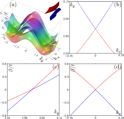
To understand the emergence of the type-II Dirac cones, we theoretically analyze the couplings among sites in Figure 1(c) by adopting the tight-binding approximation method and only considering the nearest-neighbor interaction. The corresponding Hamiltonian can be written as
| (3) |
in which , , , , , and the coupling strength. The eigenvalues of Equation (3) are the band structure, but the analytical solution is hard to obtain. Even so, one still can obtain the locations of the Dirac points, which are and between the top and middle bands, and and between the middle and bottom bands. Numerical band structure is displayed in Figure 3(a), which looks visually the same with that in Figure 2(c) although quantitatively there are difference in the value of . Since all the Dirac cones are type-II for this case, we take the Dirac point at as an example without loss of generality, and this Dirac cone is shown in the inset of Figure 3(a). Before going into a subtle theoretical analysis on this type-II Dirac cone, it is necessary to have a look at the corresponding cross sections in the plane with [Figure 3(b)], the plane with [Figure 3(c)], and the plane with [Figure 3(d)]. In the plane, the intersection of the top and middle bands, as shown in Figure 3(b), exhibits two crossing lines Soluyanov et al. (2015); Milićević et al. (2019). In Figure 3(c), the red and blue lines show the profile of the Dirac cone in the cross section which clearly elucidates that the sign of the slope does not change along direction. While in Figure 3(d), the profile of the Dirac cone in the cross section is symmetric about (i.e., sign of changes), which is similar to that for a (tilted) type-I Dirac points. To this regard, if we expand the Hamiltonian in the infinitesimal region around the Dirac point , we can only consider the component along direction and let safely. As a result, the corresponding Hamiltonian can be written as
| (4) |
The eigenvalues of this Hamiltonian are
| (5) |
Clearly, one may find the relation , which indicates that the two bands are degenerated at the point — the location of the Dirac point. One also finds that and always have the same sign, therefore the velocity does not change its sign around the Dirac point, and the Dirac cone is type-II definitely.

III Results
III.1 Conical diffraction
If the incident beam can excite the Dirac cone states properly, the beam will undergo conical diffraction during propagation Peleg et al. (2007); Ablowitz et al. (2009); Diebel et al. (2016); Leykam and Desyatnikov (2016); Zhong et al. (2017, 2019); Kang et al. (2019). Since there are type-I, type-II and type-III Dirac cones in Figure 2(b) and 2(c), we do not consider the Dirac cones in Figure 2(a) and only excite these Dirac cone states indicated by green and red circles, which can be achieved via the method developed in Refs. Zhong et al. (2019); Kang et al. (2019). After propagating a distance of , the output intensity profiles of these excited Dirac cone states are displayed in Figure 4, in which the dotted circles represent the location and size of the input Dirac cone states, and the vertical and horizontal dashed yellow lines are the and axes, respectively.
Corresponding to the tilted type-I Dirac cone surrounded by the green circle in Figure 2(b), the conical diffraction is displayed in Figure 4(a). Due to the tilt of the Dirac cone, the diffraction speed along and directions are different, so the diffraction ring exhibits an elliptic profile. If the type-III Dirac cone state is excited, as indicated by the red circle in Figure 2(b), the conical diffraction may only happen along direction, because the group velocity along direction . The numerical result is shown in Figure 4(b), and indeed, the diffraction ring only appears in the region with the location of the upper edge of the ring nearly being invariant. Different from the type-I and type-III Dirac cones, the sign of speed of the type-II Dirac cone does not change along coordinate, so the whole conical diffraction ring will move along either or direction. As to the type-II Dirac cones marked with green and red circles in Figure 2(c), conical diffraction rings will move along direction because of , and the corresponding numerical simulations are displayed in Figure 4(c) and 4(d). Considering that all the Dirac cones are tilted along coordinate only, the conical diffractions in Figure 4 are symmetric about . Note that the diameter of the diffraction ring along coordinate in Figure 4(d) is much bigger than that in Figure 4(c), and the reason is that the absolute value of of the Dirac cone surrounded by the green circle is smaller than that of the Dirac cone surrounded by the red circle. In short, the spatial conical diffraction patterns can be predicted from the profiles of the Dirac cones, and vice versa, the properties of the Dirac cones are manifested into the conical diffraction patterns.
III.2 Klein tunneling
Different from ordinary quantum mechanical tunneling, the term Klein tunneling refers to a counterintuitive relativistic process in which an electron can penetrate through a potential barrier higher than the electron’s rest energy Katsnelson et al. (2006). Since conical diffraction due to the type-II Dirac cones moves along direction spontaneously even with zero incident angle, it becomes an ideal paradigm to investigate the Klein tunneling. This is indeed more advantage than that in type-I Dirac photonic lattices, where the movement of the incident beam is required through tunning the angle of incidence. What one is required to do is setting up a barrier in the type-II Dirac photonic lattice at a proper place where the conical diffraction will move toward. Generally, the lattice potential superimposed with a barrier can be written as
| (6) |
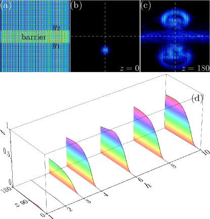
in which is the height and is the width of the barrier. The type-II Dirac photonic lattice with a barrier is shown in Figure 5(a), and the incident type-II Dirac cone state [corresponding to the Dirac cone marked with the green circle in Figure 2(c)] superimposed with a wide Gaussian that is placed below the barrier is displayed in Figure 5(b). The incident state will exhibit conical diffraction during propagation, and meanwhile, the conical diffraction pattern moves upward along direction, as in Figure 4(c). Inevitably, the conical diffraction pattern will hit on the barrier, and it will be reflected by the barrier by intuition. Nevertheless, transmission of the conical diffraction pattern over the barrier is completely possible if the barrier height is bigger than 3 – a requirement of Klein tunneling, because the “energy” of the state at the Dirac point marked with the green circle in Figure 2(c) is about . To track the Klein tunneling process, we define a physical quantity named the transmission ratio, as
with
and
The transmission ratio as a function of propagation distance for barriers with different height is shown in Figure 5(d). Distinctly, the conical diffraction is almost reflected by the barrier when the height is smaller than the “energy”; see the curves corresponding to and in Figure 5(d). Klein tunneling starts to happen if the barrier height is close to the “energy”, and this is demonstrated by the curve with . Increasing the barrier height further, the transmission ratio also grows, but numerical simulations indicate that there is seemingly a saturable value for the transmission ratio, which is . The reason for not reaching the perfect Klein tunneling is due to that the incident beam in Figure 5(b) is not really “massless”. On one hand, the Dirac cone state is approximately obtained and its corresponding Bloch momentum is not exactly in the infinitesimal region around the critical point. On the other hand, the superimposed wide Gaussian beam is a “massive” object. The output amplitude profile with is displayed in Figure 5(c), which clearly manifests the Klein tunneling of the conical diffraction. Since the conical diffraction is still hold after penetrating the barrier, excitation of the type-II Dirac cone mode is conserved.
Note that the steps of the barrier given by Equation (6) are sharp. If this barrier is replace by a barrier with smooth steps, e.g., a super-Gaussian, which transforms the potential into
with , one will not miss out on the finding that the Klein tunneling is completely inhibited, which also demonstrates that the phenomenon reported in Figure 5 is truly Klein tunneling. The explanation of this inhibition is that the barrier with smooth steps can be regarded as a combination of sub-barriers with sharp steps, infinitesimal width, and different height. The conical diffraction will first encounter the sub-barrier with very small height upon its movement along direction, and this height is always smaller than the “energy” of the conical diffraction beam which dissatisfies the requirement of appearance of the Klein tunneling.
IV Conclusion
Summarizing, we have constructed a type-II Dirac photonic lattice from the Lieb-like lattice by simply adjusting a angle parameter which only changes the spatial symmetry of the lattice. Conical diffraction and Klein tunneling in this novel type-II Dirac photonic lattice are discussed in detail. We believe that our results may not only provide a feasible avenue on light manipulation, but also help realize other topological photonic and analogize nonrelativistic phenomena in photonic lattices. In addition to photonics, we believe that the developed type-II Dirac lattice in this work may also provide a completely new flatform for cold atoms and acoustics.
Note added: A paper Wu et al. (2020) on constructing type-II Dirac points by proposing a band-folding scheme, and a paper Pyrialakos et al. (2020) on symmetry-controlled edge states in the type-II phase of Dirac photonic lattices, were published after submission of this paper. We would like to emphasize that, in our work for the first time, we find the simplest way to construct type-II Dirac points which only depends on the spatial geometry of the photonic lattice.
Acknowledgements
This work was supported by Guangdong Basic and Applied Basic Research Foundation (2018A0303130057), National Natural Science Foundation of China (U1537210, 11534008), and Fundamental Research Funds for the Central Universities (xzy012019038, xzy022019076). The authors acknowledge the computational resources provided by the HPC platform of Xi an Jiaotong University.
References
- Leykam and Desyatnikov (2016) D. Leykam and A. S. Desyatnikov, Conical intersections for light and matter waves, Adv. Phys. X 1, 101 (2016).
- Zandbergen and de Dood (2010) S. R. Zandbergen and M. J. A. de Dood, Experimental Observation of Strong Edge Effects on the Pseudodiffusive Transport of Light in Photonic Graphene, Phys. Rev. Lett. 104, 043903 (2010).
- Rechtsman et al. (2013a) M. C. Rechtsman, Y. Plotnik, J. M. Zeuner, D. Song, Z. Chen, A. Szameit, and M. Segev, Topological Creation and Destruction of Edge States in Photonic Graphene, Phys. Rev. Lett. 111, 103901 (2013a).
- Rechtsman et al. (2013b) M. C. Rechtsman, J. M. Zeuner, A. Tünnermann, S. Nolte, M. Segev, and A. Szameit, Strain-induced pseudomagnetic field and photonic Landau levels in dielectric structures, Nat. Photon. 7, 153 (2013b).
- Crespi et al. (2013) A. Crespi, G. Corrielli, G. D. Valle, R. Osellame, and S. Longhi, Dynamic band collapse in photonic graphene, New J. Phys. 15, 013012 (2013).
- Zeuner et al. (2014) J. M. Zeuner, M. C. Rechtsman, S. Nolte, and A. Szameit, Edge states in disordered photonic graphene, Opt. Lett. 39, 602 (2014).
- Plotnik et al. (2014) Y. Plotnik, M. C. Rechtsman, D. Song, M. Heinrich, J. M. Zeuner, S. Nolte, Y. Lumer, N. Malkova, J. Xu, A. Szameit, Z. Chen, and M. Segev, Observation of unconventional edge states in ‘photonic graphene’, Nat. Mater. 13, 57 (2014).
- Song et al. (2015) D. Song, V. Paltoglou, S. Liu, Y. Zhu, D. Gallardo, L. Tang, J. Xu, M. Ablowitz, N. K. Efremidis, and Z. Chen, Unveiling pseudospin and angular momentum in photonic graphene., Nat. Commun. 6, 6272 (2015).
- Nalitov et al. (2015) A. V. Nalitov, G. Malpuech, H. Terças, and D. D. Solnyshkov, Spin-Orbit Coupling and the Optical Spin Hall Effect in Photonic Graphene, Phys. Rev. Lett. 114, 026803 (2015).
- Taie et al. (2015) S. Taie, H. Ozawa, T. Ichinose, T. Nishio, S. Nakajima, and Y. Takahashi, Coherent driving and freezing of bosonic matter wave in an optical Lieb lattice, Sci. Adv. 1, 1500854 (2015).
- Vicencio et al. (2015) R. A. Vicencio, C. Cantillano, L. Morales-Inostroza, B. Real, C. Mejía-Cortés, S. Weimann, A. Szameit, and M. I. Molina, Observation of Localized States in Lieb Photonic Lattices, Phys. Rev. Lett. 114, 245503 (2015).
- Mukherjee et al. (2015) S. Mukherjee, A. Spracklen, D. Choudhury, N. Goldman, P. Öhberg, E. Andersson, and R. R. Thomson, Observation of a Localized Flat-Band State in a Photonic Lieb Lattice, Phys. Rev. Lett. 114, 245504 (2015).
- Diebel et al. (2016) F. Diebel, D. Leykam, S. Kroesen, C. Denz, and A. S. Desyatnikov, Conical Diffraction and Composite Lieb Bosons in Photonic Lattices, Phys. Rev. Lett. 116, 183902 (2016).
- Ozawa et al. (2017) H. Ozawa, S. Taie, T. Ichinose, and Y. Takahashi, Interaction-Driven Shift and Distortion of a Flat Band in an Optical Lieb Lattice, Phys. Rev. Lett. 118, 175301 (2017).
- Xia et al. (2018) S. Xia, A. Ramachandran, S. Xia, D. Li, X. Liu, L. Tang, Y. Hu, D. Song, J. Xu, D. Leykam, S. Flach, and Z. Chen, Unconventional Flatband Line States in Photonic Lieb Lattices, Phys. Rev. Lett. 121, 263902 (2018).
- El Hassan et al. (2019) A. El Hassan, F. K. Kunst, A. Moritz, G. Andler, E. J. Bergholtz, and M. Bourennane, Corner states of light in photonic waveguides, Nat. Photon. 13, 697 (2019).
- Li et al. (2019a) M. Li, D. Zhirihin, M. Gorlach, X. Ni, D. Filonov, A. Slobozhanyuk, A. Alù, and A. B. Khanikaev, Higher-order topological states in photonic kagome crystals with long-range interactions, Nat. Photon. (2019a), 10.1038/s41566-019-0561-9.
- Zhong et al. (2017) H. Zhong, Y. Q. Zhang, Y. Zhu, D. Zhang, C. B. Li, Y. P. Zhang, F. L. Li, M. R. Belić, and M. Xiao, Transport properties in the photonic super-honeycomb lattice – a hybrid fermionic and bosonic system, Ann. Phys. (Berlin) 529, 1600258 (2017).
- Kang et al. (2019) Y. F. Kang, H. Zhong, M. R. Belić, Y. Q. Tian, K. C. Jin, Y. P. Zhang, F. L. Li, and Y. Q. Zhang, Conical Diffraction from Approximate Dirac Cone States in a Superhoneycomb Lattice, Ann. Phys. (Berlin) 531, 1900295 (2019).
- Zhong et al. (2019) H. Zhong, R. Wang, M. R. Belić, Y. P. Zhang, and Y. Q. Zhang, Asymmetric conical diffraction in dislocated edge-centered square lattices, Opt. Express 27, 6300 (2019).
- Milićević et al. (2019) M. Milićević, G. Montambaux, T. Ozawa, O. Jamadi, B. Real, I. Sagnes, A. Lemaître, L. Le Gratiet, A. Harouri, J. Bloch, and A. Amo, Type-III and Tilted Dirac Cones Emerging from Flat Bands in Photonic Orbital Graphene, Phys. Rev. X 9, 031010 (2019).
- Li et al. (2019b) X.-P. Li, K. Deng, B. Fu, Y. Li, D. Ma, J. Han, J. Zhou, S. Zhou, and Y. Yao, Type-III Weyl Semimetals and its Materialization, arXiv:1909.12178 (2019b).
- Soluyanov et al. (2015) A. A. Soluyanov, D. Gresch, Z. Wang, Q. Wu, M. Troyer, X. Dai, and B. A. Bernevig, Type-II Weyl semimetals, Nature 527, 495 (2015).
- Xu et al. (2015) Y. Xu, F. Zhang, and C. Zhang, Structured Weyl Points in Spin-Orbit Coupled Fermionic Superfluids, Phys. Rev. Lett. 115, 265304 (2015).
- Chen et al. (2016) W.-J. Chen, M. Xiao, and C. T. Chan, Photonic crystals possessing multiple Weyl points and the experimental observation of robust surface states, Nat. Commun. 7, 13038 (2016).
- Autès et al. (2016) G. Autès, D. Gresch, M. Troyer, A. A. Soluyanov, and O. V. Yazyev, Robust Type-II Weyl Semimetal Phase in Transition Metal Diphosphides (, W), Phys. Rev. Lett. 117, 066402 (2016).
- Noh et al. (2017a) J. Noh, S. Huang, D. Leykam, Y. Chong, K. P. Chen, and M. Rechtsman, Experimental observation of optical Weyl points and Fermi arc-like surface states, Nat. Phys. 13, 611 (2017a).
- Chen et al. (2018) R. Chen, B. Zhou, and D.-H. Xu, Floquet Weyl semimetals in light-irradiated type-II and hybrid line-node semimetals, Phys. Rev. B 97, 155152 (2018).
- Xie et al. (2019) B. Xie, H. Liu, H. Cheng, Z. Liu, S. Chen, and J. Tian, Experimental Realization of Type-II Weyl Points and Fermi Arcs in Phononic Crystal, Phys. Rev. Lett. 122, 104302 (2019).
- Yan et al. (2017) M. Yan, H. Huang, K. Zhang, E. Wang, W. Yao, K. Deng, G. Wan, H. Zhang, M. Arita, H. Yang, Z. Sun, H. Yao, Y. Wu, S. Fan, W. Duan, and S. Zhou, Lorentz-violating type-II Dirac fermions in transition metal dichalcogenide PtTe2, Nat. Commun. 8, 257 (2017).
- Noh et al. (2017b) H.-J. Noh, J. Jeong, E.-J. Cho, K. Kim, B. I. Min, and B.-G. Park, Experimental Realization of Type-II Dirac Fermions in a Superconductor, Phys. Rev. Lett. 119, 016401 (2017b).
- Chang et al. (2017) T.-R. Chang, S.-Y. Xu, D. S. Sanchez, W.-F. Tsai, S.-M. Huang, G. Chang, C.-H. Hsu, G. Bian, I. Belopolski, Z.-M. Yu, S. A. Yang, T. Neupert, H.-T. Jeng, H. Lin, and M. Z. Hasan, Type-II Symmetry-Protected Topological Dirac Semimetals, Phys. Rev. Lett. 119, 026404 (2017).
- Fei et al. (2018) F. Fei, X. Bo, P. Wang, J. Ying, J. Li, K. Chen, Q. Dai, B. Chen, Z. Sun, M. Zhang, F. Qu, Y. Zhang, Q. Wang, X. Wang, L. Cao, H. Bu, F. Song, X. Wan, and B. Wang, Band Structure Perfection and Superconductivity in Type-II Dirac Semimetal Ir1-xPtxTe2, Adv. Mater. 30, 1801556 (2018).
- Politano et al. (2018) A. Politano, G. Chiarello, B. Ghosh, K. Sadhukhan, C.-N. Kuo, C. S. Lue, V. Pellegrini, and A. Agarwal, 3D Dirac Plasmons in the Type-II Dirac Semimetal , Phys. Rev. Lett. 121, 086804 (2018).
- Kim et al. (2018) D. Kim, S. Ahn, J. H. Jung, H. Min, J. Ihm, J. H. Han, and Y. Kim, Type-II Dirac line node in strained , Phys. Rev. Mater. 2, 104203 (2018).
- Wang et al. (2018) B. Wang, H. Gao, Q. Lu, W. Xie, Y. Ge, Y.-H. Zhao, K. Zhang, and Y. Liu, Type-I and type-II nodal lines coexistence in the antiferromagnetic monolayer , Phys. Rev. B 98, 115164 (2018).
- Lin et al. (2017) J. Y. Lin, N. C. Hu, Y. J. Chen, C. H. Lee, and X. Zhang, Line nodes, Dirac points, and Lifshitz transition in two-dimensional nonsymmorphic photonic crystals, Phys. Rev. B 96, 075438 (2017).
- Pyrialakos et al. (2017) G. G. Pyrialakos, N. S. Nye, N. V. Kantartzis, and D. N. Christodoulides, Emergence of Type-II Dirac Points in Graphynelike Photonic Lattices, Phys. Rev. Lett. 119, 113901 (2017).
- Wang et al. (2017) H.-X. Wang, Y. Chen, Z. H. Hang, H.-Y. Kee, and J.-H. Jiang, Type-II Dirac photons, npj Quant. Mater. 2, 54 (2017).
- Hu et al. (2018) C. Hu, Z. Li, R. Tong, X. Wu, Z. Xia, L. Wang, S. Li, Y. Huang, S. Wang, B. Hou, C. T. Chan, and W. Wen, Type-II Dirac Photons at Metasurfaces, Phys. Rev. Lett. 121, 024301 (2018).
- Mann et al. (2018) C.-R. Mann, T. J. Sturges, G. Weick, W. L. Barnes, and E. Mariani, Manipulating type-I and type-II Dirac polaritons in cavity-embedded honeycomb metasurfaces, Nat. Commun. 9, 2194 (2018).
- Li et al. (2017) S. Li, Z.-M. Yu, Y. Liu, S. Guan, S.-S. Wang, X. Zhang, Y. Yao, and S. A. Yang, Type-II nodal loops: Theory and material realization, Phys. Rev. B 96, 081106 (2017).
- Katsnelson et al. (2006) M. I. Katsnelson, K. S. Novoselov, and A. K. Geim, Chiral tunnelling and the Klein paradox in graphene, Nat. Phys. 2, 620 (2006).
- Bahat-Treidel et al. (2010) O. Bahat-Treidel, O. Peleg, M. Grobman, N. Shapira, M. Segev, and T. Pereg-Barnea, Klein Tunneling in Deformed Honeycomb Lattices, Phys. Rev. Lett. 104, 063901 (2010).
- Bahat-Treidel and Segev (2011) O. Bahat-Treidel and M. Segev, Nonlinear wave dynamics in honeycomb lattices, Phys. Rev. A 84, 021802 (2011).
- Longhi (2010) S. Longhi, Klein tunneling in binary photonic superlattices, Phys. Rev. B 81, 075102 (2010).
- Dreisow et al. (2012) F. Dreisow, R. Keil, A. Tünnermann, S. Nolte, S. Longhi, and A. Szameit, Klein tunneling of light in waveguide superlattices, EPL 97, 10008 (2012).
- Sun et al. (2017) L. Sun, J. Gao, and X. Yang, Klein tunneling near the Dirac points in metal-dielectric multilayer metamaterials, Sci. Rep. 7, 9678 (2017).
- Fang et al. (2019) A. Fang, Z. Q. Zhang, S. G. Louie, and C. T. Chan, Pseudospin-1 Physics of Photonic Crystals, Research 2019, 3054062 (2019).
- Li et al. (2018) C. Li, F. Ye, X. Chen, Y. V. Kartashov, A. Ferrando, L. Torner, and D. V. Skryabin, Lieb polariton topological insulators, Phys. Rev. B 97, 081103 (2018).
- Rechtsman et al. (2013c) M. C. Rechtsman, J. M. Zeuner, Y. Plotnik, Y. Lumer, D. Podolsky, F. Dreisow, S. Nolte, M. Segev, and A. Szameit, Photonic Floquet topological insulators, Nature 496, 196 (2013c).
- Stützer et al. (2018) S. Stützer, Y. Plotnik, Y. Lumer, P. Titum, N. H. Lindner, M. Segev, M. C. Rechtsman, and A. Szameit, Photonic topological Anderson insulators, Nature 560, 461 (2018).
- Lustig et al. (2019) E. Lustig, S. Weimann, Y. Plotnik, Y. Lumer, M. A. Bandres, A. Szameit, and M. Segev, Photonic topological insulator in synthetic dimensions, Nature 567, 356 (2019).
- Wang et al. (2020) P. Wang, Y. Zheng, X. Chen, C. Huang, Y. V. Kartashov, L. Torner, V. V. Konotop, and F. Ye, Localization and delocalization of light in photonic moiré lattices, Nature 577, 42 (2020).
- Tarruell et al. (2012) L. Tarruell, D. Greif, T. Uehlinger, G. Jotzu, and T. Esslinger, Creating, moving and merging Dirac points with a Fermi gas in a tunable honeycomb lattice, Nature 483, 302 (2012).
- Bartal et al. (2005) G. Bartal, O. Cohen, H. Buljan, J. W. Fleischer, O. Manela, and M. Segev, Brillouin Zone Spectroscopy of Nonlinear Photonic Lattices, Phys. Rev. Lett. 94, 163902 (2005).
- Peleg et al. (2007) O. Peleg, G. Bartal, B. Freedman, O. Manela, M. Segev, and D. N. Christodoulides, Conical Diffraction and Gap Solitons in Honeycomb Photonic Lattices, Phys. Rev. Lett. 98, 103901 (2007).
- Ablowitz et al. (2009) M. J. Ablowitz, S. D. Nixon, and Y. Zhu, Conical diffraction in honeycomb lattices, Phys. Rev. A 79, 053830 (2009).
- Wu et al. (2020) X. Wu, X. Li, R.-Y. Zhang, X. Xiang, J. Tian, Y. Huang, S. Wang, B. Hou, C. T. Chan, and W. Wen, Deterministic Scheme for Two-Dimensional Type-II Dirac Points and Experimental Realization in Acoustics, Phys. Rev. Lett. 124, 075501 (2020).
- Pyrialakos et al. (2020) G. G. Pyrialakos, N. Schmitt, N. S. Nye, M. Heinrich, N. V. Kantartzis, A. Szameit, and D. N. Christodoulides, Symmetry-controlled edge states in the type-II phase of Dirac photonic lattices, Nat. Commun. 11, 2074 (2020).