This paper was converted on www.awesomepapers.org from LaTeX by an anonymous user.
Want to know more? Visit the Converter page.

Two-Stage Channel Estimation Approach for Cell-Free IoT With Massive Random Access

Xinhua Wang, Member, IEEE, Alexei Ashikhmin, Fellow, IEEE, Zhicheng Dong, Member, IEEE, and Chao Zhai, Member, IEEE Copyright (c) 2015 IEEE. Personal use of this material is permitted. However, permission to use this material for any other purposes must be obtained from the IEEE by sending a request to [email protected]. X. Wang is with the College of Electrical Engineering, Qingdao University, Qingdao, 266071 China (e-mail: [email protected]). A. Ashikhmin is with the Nokia Bell Labs, Murray Hill, NJ 07974 USA (e-mail: [email protected]). Z. Dong is with the School of Engineering, Tibet University, Lhasa, 850000 China (e-mail: [email protected]). C. Zhai is with the School of Information Science and Engineering, Shandong University, Qingdao, 266237 China (e-mail: [email protected]).
Abstract

We investigate the activity detection and channel estimation issues for cell-free Internet of Things (IoT) networks with massive random access. In each time slot, only partial devices are active and communicate with neighboring access points (APs) using non-orthogonal random pilot sequences. Different from the centralized processing in cellular networks, the activity detection and channel estimation in cell-free IoT is more challenging due to the distributed and user-centric architecture. We propose a two-stage approach to detect the random activities of devices and estimate their channel states. In the first stage, the activity of each device is jointly detected by its adjacent APs based on the vector approximate message passing (Vector AMP) algorithm. In the second stage, each AP re-estimates the channel using the linear minimum mean square error (LMMSE) method based on the detected activities to improve the channel estimation accuracy. We derive closed-form expressions for the activity detection error probability and the mean-squared channel estimation errors for a typical device. Finally, we analyze the performance of the entire cell-free IoT network in terms of coverage probability. Simulation results validate the derived closed-form expressions and show that the cell-free IoT significantly outperforms the collocated massive MIMO and small-cell schemes in terms of coverage probability.

Index Terms:
Approximate message passing, cell-free IoT networks, joint activity detection and channel estimation, massive random access, two-stage channel estimation.

I Introduction

Internet of Things (IoT) is a promising technology to enable massively connected intelligent objects to make decisions cooperatively. IoT has been wildly exploited in many fields, such as smart healthcare and intelligent transportation, which can bring revolutionary changes to our daily life [1]. With the increasing development of IoT, the number of machine-type connections has grown exponentially with a rate of tens of billions a year [2]. Different with human-driven communications, the data traffic of machine-type communications (MTC) is often light, but requires random access to the network. Typically, in each given time slot, only a small fraction of devices are active, which shows the nature of sparsity [3].

In order to support the massive connectivity, a number of coordinated access and user scheduling schemes have been proposed [4, 5]. Hasan et al. proposed a random access mechanism similarly as the classic ALOHA, wherein each active device first randomly selects a pilot sequence from a finite set and transmits it to notify the base station (BS) about its status [4]. After receiving the response from a BS, the active device sends a data transmission request, which may be denied if it picks the same pilot sequence with another active device. With the help of Lyapunov optimization, Zhai et al. designed an energy-efficient user scheduling and power allocation scheme for the NOMA based IoT, which aims to minimize the network power consumption while meeting the long-term rate requirements of all the devices [5]. Unfortunately, the extra control signaling significantly increases the overhead of IoT networks, which may be even heaver than the data traffic.

Apart from the grant-based access schemes mentioned above, the grant-free IoT with random pilots has also been attracting intensive research interests, as each device can directly transmit its pilot and data to the BS without waiting for any permission [6]. Thanks to the sparsity of active users, the compressed sensing (CS) techniques can be adopted for the activity detection. With perfect channel state information (CSI) available, a block-wise orthogonal least-squares detection was proposed in [7] to jointly detect user activity and data. Leveraging the Gaussian distribution of random pilots, the approximate message passing (AMP) algorithm can be used to jointly detect the user activity and estimate the CSI. For a single BS with single antenna, the joint activity and channel estimation problem becomes a CS single measurement vector problem, which can be efficiently solved using the AMP algorithm [8]. For a single BS with multiple antennas, a CS multiple measurement vector problem can be formulated as in [9], which can be solved using the similar arguments. Through asymptotic analysis, the detection error probability of the AMP-based algorithm were derived for a single-cell massive MIMO system in [10]. Due to the severe path-loss, cell-boundary devices often suffer from very poor detection probability.

Recently, cell-free massive MIMO has been proposed as a promising technique for the next-generation wireless systems with many distributed APs cooperatively transmitting data [11]. In contrast to cellular networks, each user is served jointly by neighboring APs [12]. As a result, the severe path-loss effect can be alleviated in the distributed and user-centric architecture [13]. In order to acquire the CSI, each AP can locally estimate the CSI using the linear minimum mean square error (LMMSE) technique. Considering the massive connectivity in IoT networks, the optimal LMMSE channel estimation with non-orthogonal random pilots were studied in [14] and [15] for single and multiple antenna cases, respectively. Using the local CSI, each AP pre-processes the received signals separately, and then delivers the generated scalars to the CPU for the combination and decoding. In all of these works, it is assumed that the active users are all correctly identified, thus APs need to estimate the channel coefficients of all the active users. This assumption is not suitable for the grant-free IoT networks with massive connectivity.

In this work, we consider a user-centric and distributed cell-free network, wherein each device is served by all the APs located in a circular area with a given radius around the device. Activity detection in cell-free networks is a challenging problem, because the previously used CS techniques require centralized processing at the cellular BS, which is not suitable for the user-centric cell-free network [16]. Inspired by this fact, we propose a two-stage approach to detect active users and estimate their channel coefficients, and further analyze the system performance. Our main contributions are three-fold:

  • We properly model the stochastic cell-free IoT network with massive random access in the 2\mathbb{R}^{2} regime. We propose a two-stage approach to detect active users and estimate their channel coefficients. In the first stage, the activity of each device is jointly determined by its adjacent APs based on the vector AMP algorithm. In the second stage, the APs re-estimate the CSI using the low-complexity LMMSE method to improve the accuracy of CSI estimation for the active users.

  • For each device, we derive closed-form expressions for the activity detection error probability and the mean-squared channel estimation error through asymptotic analysis. Furthermore, we study the impact of the number of antennas applied at each AP, and the density of APs.

  • For the entire stochastic network, we analyze the coverage probability and make comparisons with the cellular massive MIMO and small-cells. Simulation results verify the accuracy of the derived closed-form expressions and show that the user-centric approach can significantly improve the accuracy of channel estimation.

The rest of this paper is organized as follows. In Section II, we describe the system model and outline our results. In Section III, we illustrate the proposed two-stage approach. Section IV and V analyze the performance of device and network, respectively. Simulation results are provided in Section VI. Finally, Section VII concludes this paper.

Notation: Throughout this paper, scalars and vectors are denoted by lowercase letters and boldface lowercase letters, respectively. ||\left|\cdot\right| and \left\|\cdot\right\| represent the absolute value and the 2\ell_{2} norm, respectively. ()H(\cdot)^{H} and ()1(\cdot)^{-1} denote the conjugate transpose and the inverse operation, respectively. 𝒞𝒩(m,R)\mathcal{CN}\left(\textbf{m},\textbf{R}\right) denotes the circularly symmetric complex Gaussian (CSCG) distribution with mean vector m and covariance matrix R. 𝔼[]\mathbb{E}[\cdot] and var{}\{\cdot\} stand for expectation and variance operations, respectively. Γ()\Gamma(\cdot), γ(,)\gamma(\cdot,\cdot), Γ(,)\Gamma(\cdot,\cdot) denote the Gamma function, the lower incomplete Gamma function, and the upper incomplete Gamma function, respectively. xGamma(a,b)x\sim{\rm Gamma}(a,b) represents that a random variable xx is gamma-distributed with shape aa and scale bb.

II System Model and Outline of Results

Refer to caption
Figure 1: The stochastic cell-free IoT network with massive random access. The gray circle with radius R0R_{0} is the coverage area of the mm-th AP, and 𝒟m\mathcal{D}_{m} is the set of the devices within the gray circle. The red circle with radius R0R_{0} is the coverage area of the kk-th device, and 𝒜k\mathcal{A}_{k} is the set of the APs within the red circle. The activity of the kk-th device is jointly determined by the APs denoted as 𝒜~k\widetilde{\mathcal{A}}_{k} within the green circle with cooperation radius R1<R0R_{1}<R_{0}.

II-A System Model

As shown in Fig. 1, we consider a stochastic user-centric cell-free IoT network, which consists of randomly distributed APs and IoT devices. Each AP is equipped with NN antennas and connects to a central processing unit (CPU), via a back-haul network. We assume that the locations of APs follow a homogeneous Poisson point process (PPP) ΦA{\Phi}_{A} with density λA\lambda_{\rm A}, while the locations of devices follow another independent homogeneous PPP ΦD{\Phi}_{D} with higher density λD\lambda_{\rm D}\rightarrow\infty. In each time slot, each device independently transmit data to APs with probability ϵ\epsilon. Let rm,kr_{m,k} denote the distance between the mm-th AP and the kk-th device. Let 𝒈m,kN×1{\boldsymbol{g}}_{m,k}\in\mathbb{C}^{N\times 1} denote the corresponding channel coefficients. Unlike a cellular network, each device is served by its adjacent APs within its coverage area. Here, the coverage area of each AP or each device is a circular area with sufficient large radius R0R_{0}. The nn-th element of 𝒈m,k{\boldsymbol{g}}_{m,k} is modeled as

g(m,n),k={βm,kh(m,n),k,ifrm,kR0,0,otherwise,\displaystyle g_{(m,n),k}=\left\{\begin{array}[]{ll}\sqrt{\beta_{m,k}}h_{(m,n),k},&{\rm if}~{}r_{{m},k}\leq R_{0},\\ 0,&\mbox{otherwise},\end{array}\right.

where h(m,n),k𝒞𝒩(0,1)h_{(m,n),k}\sim\mathcal{CN}(0,1) is the small-scale fading, and βm,k\sqrt{\beta_{m,k}} denotes the path-loss which decreases monotonically with rm,kr_{m,k}. As shown in Fig. 1, the kk-th device is served by a set of APs denoted by 𝒜k\mathcal{A}_{k}, which are located within its coverage area denoted by a red circle. Let 𝒟m\mathcal{D}_{m} be the set of devices within the coverage area of the mm-th AP denoted by the gray circle.

Let αk\alpha_{k} be the activity indicator of the kk-th device, i.e.,

αk={1,ifk-th device is active,0,otherwise.\displaystyle{\alpha}_{k}=\left\{\begin{array}[]{ll}1,&{\rm if}~{}k\mbox{-th device is active},\\ 0,&\mbox{otherwise}.\end{array}\right. (3)

Let Pr(αk=1)=ϵ,k{\Pr}(\alpha_{k}=1)=\epsilon,\forall k. We assume that the activity detection for the kk-th device is conducted by APs located within the circular area of radius R1R0R_{1}\leq R_{0} (the green circle in Fig. 1). We call R1R_{1} the cooperative radius. We denote the cooperative APs by the set 𝒜~k={m:rm,kR1}\widetilde{\mathcal{A}}_{k}=\{m:r_{m,k}\leq R_{1}\}.

In the channel estimation phase, each active device transmits the pilot sequence 𝝍k𝒞𝒩(0,1τ𝑰τ)\boldsymbol{\psi}_{k}\sim\mathcal{CN}\left(0,\frac{1}{\tau}{\boldsymbol{I}}_{\tau}\right) with a normalized power ρ\rho, where τ\tau is the length of each pilot sequence. For the mm-th AP, we define 𝜶m=diag(,αk,){\boldsymbol{\alpha}}_{m}={\rm diag}(\cdots,\alpha_{k},\cdots), 𝜷m=diag(,βm,k,){\boldsymbol{\beta}}_{m}={\rm diag}(\cdots,\beta_{m,k},\cdots), and 𝚿m=[,𝝍k,]τ×|𝒟m|\boldsymbol{\Psi}_{m}=\left[\cdots,\boldsymbol{\psi}_{k},\cdots\right]\sim\mathbb{C}^{\tau\times|\mathcal{D}_{m}|} where k𝒟mk\in\mathcal{D}_{m}, and 𝚿m\boldsymbol{\Psi}_{m} and 𝜷m{\boldsymbol{\beta}}_{m} are assumed to be available for the mm-th AP. Let E=τρE=\tau\rho, the received signal at the nn-th antenna of the mm-th AP is given by

𝒚(m,n)\displaystyle\boldsymbol{y}_{(m,n)} =Ek𝒟mαkg(m,n),k𝝍k+𝒘(m,n)\displaystyle=\sqrt{E}\sum\nolimits_{k\in\mathcal{D}_{m}}\alpha_{k}{g}_{(m,n),k}\boldsymbol{\psi}_{k}+{\boldsymbol{w}}_{(m,n)}
=E𝚿m𝜶m𝒈(m,n)+𝒘(m,n),\displaystyle=\sqrt{E}\boldsymbol{\Psi}_{m}{\boldsymbol{\alpha}}_{m}\boldsymbol{g}_{(m,n)}+{\boldsymbol{w}}_{(m,n)}, (4)

where 𝒘(m,n)𝒞𝒩(0,𝑰τ){\boldsymbol{w}}_{(m,n)}\sim\mathcal{CN}(0,\boldsymbol{I}_{\tau}) is the normalized noise, and

𝒈(m,n)=[,g(m,n),k,]T|𝒟m|×1,k𝒟m\displaystyle\boldsymbol{g}_{(m,n)}=\left[\cdots,g_{(m,n),k},\cdots\right]^{T}~{}\in\mathbb{C}^{|\mathcal{D}_{m}|\times 1},~{}k\in\mathcal{D}_{m}

denotes the channel coefficients vector between the nn-th antenna of the mm-th AP and the devices in 𝒟m\mathcal{D}_{m}. The channel coefficients between the mm-th AP and the kk-th device are given by

𝒈m,k=[g(m,1),k,,g(m,N),k]TN×1,k𝒟m,\displaystyle\boldsymbol{g}_{m,k}=\left[g_{(m,1),k},\cdots,g_{(m,N),k}\right]^{T}~{}\in\mathbb{C}^{N\times 1},~{}k\in\mathcal{D}_{m}, (5)

with 𝒈m,k𝒞𝒩(0,βm,k𝑰N),k𝒟m\boldsymbol{g}_{m,k}\sim\mathcal{CN}(0,\beta_{m,k}{\boldsymbol{I}}_{N}),~{}k\in\mathcal{D}_{m}. We combine the channel coefficients between all the NN antennas of the mm-th AP and all the devices in 𝒟m\mathcal{D}_{m} into the matrix

𝑮m=[𝒈(m,1),,𝒈(m,N)]=[,𝒈m,k,]T,k𝒟m.{\boldsymbol{G}}_{m}=[{{\boldsymbol{g}}}_{(m,1)},\cdots,\boldsymbol{g}_{(m,N)}]=[\cdots,{{\boldsymbol{g}}}_{m,k},\cdots]^{T},~{}k\in\mathcal{D}_{m}.

According to (4), the received pilots at the mm-th AP can be expressed as

𝒀m\displaystyle\boldsymbol{Y}_{m} =E𝚿m𝜶m𝑮m+𝑾m=E𝚿m𝑿m+𝑾m,\displaystyle=\sqrt{E}\boldsymbol{\Psi}_{m}\boldsymbol{\alpha}_{m}\boldsymbol{G}_{m}+{\boldsymbol{W}}_{m}=\sqrt{E}\boldsymbol{\Psi}_{m}\boldsymbol{X}_{m}+{\boldsymbol{W}}_{m}, (6)

where

𝒀m=[𝒚(m,1),,𝒚(m,N)],\boldsymbol{Y}_{m}=[\boldsymbol{y}_{(m,1)},\cdots,\boldsymbol{y}_{(m,N)}],
𝑾m=[𝒘(m,1),,𝒘(m,N)],\boldsymbol{W}_{m}=[\boldsymbol{w}_{(m,1)},\cdots,\boldsymbol{w}_{(m,N)}],

and

𝑿m=𝜶m𝑮m=[,𝒙m,k,]T,k𝒟m,\boldsymbol{X}_{m}=\boldsymbol{\alpha}_{m}\boldsymbol{G}_{m}=[\cdots,\boldsymbol{x}_{m,k},\cdots]^{T},~{}k\in\mathcal{D}_{m},

with

𝒙m,k=αk𝒈m,k.\displaystyle{\boldsymbol{x}}_{m,k}=\alpha_{k}{\boldsymbol{g}}_{m,k}. (7)

According to (3), the distribution of 𝒙m,k{\boldsymbol{x}}_{m,k} is

p𝒙m,k=(1ϵ)δ𝟎+ϵp𝒈m,k,p_{{\boldsymbol{x}}_{m,k}}=(1-\epsilon)\delta_{\bf 0}+\epsilon p_{{\boldsymbol{g}}_{m,k}}, (8)

where δ𝟎\delta_{\bf 0} denotes the point mass measure at zero as the kk-th device is inactive, and p𝒈m,kp_{{\boldsymbol{g}}_{m,k}} is the probability density function (PDF) of 𝒈m,k\boldsymbol{g}_{m,k} defined in (5).

For the ease of understanding, some notations of this paper are summarized in Table I. To facilitate analysis, we have the following assumptions made throughout this paper:

  • We consider the cell-free IoT with massive connectivity, i.e., λD\lambda_{D}\rightarrow\infty, which implies the number of active devices within the coverage of mm-th AP |Ωm|/|𝒟m|ϵ|\Omega_{m}|/|\mathcal{D}_{m}|\rightarrow\epsilon,  m\forall m.

  • Similar to [10], we consider the asymptotic regime with T,τ,|𝒟m|T,\tau,|\mathcal{D}_{m}|\rightarrow\infty, while keeping the total transmit energy of pilot E=τρE=\tau\rho, and the ratios τ/T\tau/T and τ/|𝒟m|\tau/|\mathcal{D}_{m}| fixed.

TABLE I:
Notation Meaning
ΦA\Phi_{A} Poisson point process (PPP) of APs
λA\lambda_{A} Density of ΦA\Phi_{A}
ΦD\Phi_{D} PPP of devices
λD\lambda_{D} Density of ΦD\Phi_{D}
rm,kr_{m,k} Distance between the mm-th AP and the kk-th device
αk\alpha_{k} Activity indicator of the kk-th device
α^k\widehat{\alpha}_{k} estimate of αk\alpha_{k}
𝝍k{\boldsymbol{\psi}}_{k} Pilot sequence of the kk-th device
τ\tau Length of pilot
EE Total transmit energy of pilot, i.e., E=τρE=\tau\rho
ρ\rho Normalized pilot transmit power
R0R_{0} Coverage radius
R1R_{1} Cooperation radius
𝒜k\mathcal{A}_{k} Set of APs within the coverage radius of the kk-th device, i.e., 𝒜k={m:rm,kR0}\mathcal{A}_{k}=\{m:r_{m,k}\leq R_{0}\}.
𝒜~k\widetilde{\mathcal{A}}_{k} Set of APs to jointly determine αk\alpha_{k}, i.e., 𝒜~k={m:rm,kR1}\widetilde{\mathcal{A}}_{k}=\{m:r_{m,k}\leq R_{1}\}
𝒟m\mathcal{D}_{m} Set of devices within the coverage radius of the mm-th AP, i.e., 𝒟m={k:dm,kR0}{\mathcal{D}}_{m}=\{k:d_{m,k}\leq R_{0}\}
Ωm\Omega_{m} Active devices within the coverage radius of the mm-th AP, i.e., Ωm={k:αk=1,k𝒟m}\Omega_{m}=\{k:\alpha_{k}=1,k\in{\mathcal{D}}_{m}\}

For the mm-th AP, the path-loss coefficients βm,k,k𝒟m\beta_{m,k},k\in\mathcal{D}_{m} follow independent identical distribution for different geometry realizations, i.e., βm,kpβ,k𝒟m\beta_{m,k}\sim p_{\beta},\forall k\in\mathcal{D}_{m}. For a snap shot, each geometry realization of {βm,k:k𝒟m}\{\beta_{m,k}:k\in\mathcal{D}_{m}\} is equivalent to |𝒟m||\mathcal{D}_{m}| multiplied by the realization of any βm,k\beta_{m,k} with k𝒟mk\in\mathcal{D}_{m}. Thus, the PDF of each geometry realization of {βm,k:k𝒟m}\{\beta_{m,k}:k\in\mathcal{D}_{m}\} converges to pβp_{\beta} as λD\lambda_{D}\rightarrow\infty.

II-B Outline of Results

For the distributed and user-centric architecture, it is nontrivial to detect the user activity and estimate the CSI for cell-free IoT networks due to the following reasons: (1) The activity αk\alpha_{k} is jointly determined by its adjacent APs, which means the traditional centralized detection techniques [10] for cellular networks are unavailable. (2) Considering the overhead over back-haul, the distributed APs cannot fully cooperate to detect user activities. (3) Compared with [15], the performance analysis for LMMSE channel estimation is more challenging due to the possible errors of activity detection.

In Section III, we will propose a two-stage channel estimation approach based on the AMP algorithm and the LMMSE method.

  • Stage I: According to the signals 𝒀m\boldsymbol{Y}_{m} defined in (6), each AP first estimates 𝑿m\boldsymbol{X}_{m} using the AMP algorithm. Then, the activity α^k\widehat{\alpha}_{k} of the kk-th device is jointly determined by fusing the estimates {𝒙^m,k:m𝒜~k}\{\widehat{\boldsymbol{x}}_{m,k}:m\in\widetilde{\mathcal{A}}_{k}\} from the adjacent APs 𝒜~k\widetilde{\mathcal{A}}_{k}.

  • Stage II: The channel vectors {𝒈^m,k:k𝒟m}\{\widehat{\boldsymbol{g}}_{m,k}:k\in\mathcal{D}_{m}\} are re-estimated by the mm-th AP using the low-complexity LMMSE method based on 𝜶^m=diag(,αk,),k𝒟m\widehat{\boldsymbol{\alpha}}_{m}={\rm diag}(\cdots,\alpha_{k},\cdots),k\in\mathcal{D}_{m} and 𝒀m\boldsymbol{Y}_{m}.

In Section IV, the activity detection error probability and the mean-squared error of channel estimate are derived in closed-form using the asymptotic analysis. In addition, we investigate how the number of antennas and the density of APs affect the system performance.

In Section V, we define the coverage probability as a metric to evaluate the performance for the entire stochastic cell-free IoT network. Then, we compare our user-centric based channel estimation approach with the collocated massive MIMO and small-cell in terms of coverage probability .

III Two-stage Channel Estimation Approach

III-A Pre-processing at Each AP for Stage I

First, the mm-th AP independently estimates 𝑿m\boldsymbol{X}_{m} based on 𝒀m\boldsymbol{Y}_{m} using the vector AMP algorithm. Similarly to [10], the vector AMP algorithm is updated as follows with initialization 𝑿m,(0)=𝟎\boldsymbol{X}_{m,{(0)}}=\boldsymbol{0} and 𝑹m,(0)=𝒀m\boldsymbol{R}_{m,{(0)}}=\boldsymbol{Y}_{m},

𝒙m,k,(t+1)\displaystyle\boldsymbol{x}_{{m,k},{(t+1)}} =η(𝒙^m,k,(t)),k𝒟m,\displaystyle=\eta\left(\widehat{\boldsymbol{x}}_{{m,k},{(t)}}\right),k\in\mathcal{D}_{m}, (9)
𝑹m,(t+1)\displaystyle\boldsymbol{R}_{m,{(t+1)}} =𝒀m𝚿m𝑿m,(t+1)\displaystyle=\boldsymbol{Y}_{m}-\boldsymbol{\Psi}_{m}\boldsymbol{X}_{m,{(t+1)}}
+|𝒟m|τ𝑹m,(t)k𝒟mη(𝒙^m,k,(t))|𝒟m|,\displaystyle+\frac{|\mathcal{D}_{m}|}{\tau}\boldsymbol{R}_{m,{(t)}}\sum\nolimits_{k\in\mathcal{D}_{m}}\frac{\eta^{\prime}(\widehat{\boldsymbol{x}}_{{m,k},{(t)})}}{|\mathcal{D}_{m}|}, (10)

where t=0,1,t=0,1,\cdots is the index of iteration, and

𝒙^m,k,(t)=𝑹m,(t)H𝝍m,k+𝒙m,k,(t).\widehat{\boldsymbol{x}}_{{m,k},{(t)}}=\boldsymbol{R}_{m,{(t)}}^{H}\boldsymbol{\psi}_{m,k}+\boldsymbol{x}_{{m,k},{(t)}}.

𝑿m,(t)=[,𝒙m,k,(t),]T,k𝒟m\boldsymbol{X}_{m,{(t)}}=[\cdots,\boldsymbol{x}_{{m,k},{(t)}},\cdots]^{T},~{}k\in\mathcal{D}_{m} is the estimate of 𝑿m\boldsymbol{X}_{m} at the tt-th iteration, and 𝑹m,(t)=[,𝒓m,k,(t),]T,k𝒟m\boldsymbol{R}_{m,{(t)}}=[\cdots,\boldsymbol{r}_{{m,k},{(t)}},\cdots]^{T},~{}k\in\mathcal{D}_{m} represents the corresponding residual. η()\eta(\cdot) and η()\eta^{\prime}(\cdot) represent an appropriately designed denoiser and its first-order derivative, respectively. Using the state evolution [10], 𝒙^m,k,(t)\widehat{\boldsymbol{x}}_{{m,k},{(t)}} can be modeled as signal 𝒙m,k\boldsymbol{x}_{m,k} plus independent Gaussian noise 𝒗m,k𝒞𝒩(0,𝑰N)\boldsymbol{v}_{m,k}\sim\mathcal{CN}(\textbf{0},{\boldsymbol{I}}_{N}), i.e.,

𝒙^m,k,(t)=𝒙m,k+𝚯m,(t)12𝒗m,k,\displaystyle\widehat{\boldsymbol{x}}_{{m,k},{(t)}}=\boldsymbol{x}_{m,k}+\boldsymbol{\Theta}_{m,{(t)}}^{\frac{1}{2}}\boldsymbol{v}_{m,k}, (11)

where 𝒗m,k\boldsymbol{v}_{m,k} is independent of 𝒙m,k\boldsymbol{x}_{m,k}, and the state 𝚯m,(t)\boldsymbol{\Theta}_{m,{(t)}} can be predicted according to the state evolution. Starting from the initial state

𝚯m,(0)=𝑰E+|𝒟m|τ𝔼𝒟m[𝑿m,k𝑿m,kH],\displaystyle\boldsymbol{\Theta}_{m,{(0)}}=\frac{\boldsymbol{I}}{E}+\frac{|\mathcal{D}_{m}|}{\tau}\mathbb{E}_{\mathcal{D}_{m}}\bigg{[}\boldsymbol{X}_{m,k}\boldsymbol{X}_{m,k}^{H}\bigg{]}, (12)

the state evolution of the AMP algorithm at each iteration is updated as [10], i.e.,

𝚯m,(t+1)=𝑰E+\displaystyle\boldsymbol{\Theta}_{m,{(t+1)}}=\frac{\boldsymbol{I}}{E}+ |𝒟m|τ𝔼𝒟m{[η(𝑿^m,k,(t))𝑿m,k]\displaystyle\frac{|\mathcal{D}_{m}|}{\tau}\mathbb{E}_{\mathcal{D}_{m}}\left\{\left[\eta(\widehat{\boldsymbol{X}}_{{m,k},{(t)}})-\boldsymbol{X}_{m,k}\right]\right.
[η(𝑿^m,k,(t))𝑿m,k]H},\displaystyle\qquad\qquad\left.\left[\eta(\widehat{\boldsymbol{X}}_{{m,k},{(t)}})-\boldsymbol{X}_{m,k}\right]^{H}\right\}, (13)

where 𝑿m,k\boldsymbol{X}_{m,k}, 𝑽m,k\boldsymbol{V}_{m,k} and 𝑿^m,k,(t)=𝑿m,k+𝚯m,(t)12𝑽m,k\widehat{\boldsymbol{X}}_{{m,k},{(t)}}=\boldsymbol{X}_{m,k}+\boldsymbol{\Theta}_{m,{(t)}}^{\frac{1}{2}}\boldsymbol{V}_{m,k} are used to capture the distribution of 𝒙m,k\boldsymbol{x}_{m,k}, 𝒗m,k\boldsymbol{v}_{m,k}, and 𝒙^m,k,(t)\widehat{\boldsymbol{x}}_{{m,k},{(t)}}, respectively. The expectation is taken over all of the devices in 𝒟m\mathcal{D}_{m}.

For a given 𝒙^m,k,(t)\widehat{\boldsymbol{x}}_{{m,k},{(t)}}, the MMSE denoiser η()\eta(\cdot) is designed the same as in [10], given by

η(𝒙^m,k,(t))=𝔼[𝑿m,k|𝑿^m,k,(t)=𝒙^m,k,(t)]\displaystyle\eta(\widehat{\boldsymbol{x}}_{{m,k},{(t)}})=\mathbb{E}\left[{{\boldsymbol{X}}}_{m,k}|\widehat{{\boldsymbol{X}}}_{{m,k},{(t)}}=\widehat{{\boldsymbol{x}}}_{{m,k},{(t)}}\right]
=ϕm,k,(t)βm,k(βm,k𝑰+𝚯m,(t))1𝒙^m,k,(t),\displaystyle=\phi_{{m,k},{(t)}}\beta_{m,k}\left(\beta_{m,k}{\boldsymbol{I}}+{\boldsymbol{\Theta}}_{m,{(t)}}\right)^{-1}\widehat{{\boldsymbol{x}}}_{{m,k},{(t)}}, (14)

where

ϕm,k,(t)=11+1ϵϵexp[N(μm,k,(t)νm,k,(t))],\displaystyle\phi_{{m,k},{(t)}}=\frac{1}{{1+\frac{1-\epsilon}{\epsilon}{\rm exp}\left[-N(\mu_{{m,k},{(t)}}-\nu_{{m,k},{(t)}})\right]}}, (14a)
μm,k,(t)=1N𝒙^m,k,(t)H{𝚯m,(t)1[βm,k𝑰+𝚯m,(t)]1}𝒙^m,k,(t),\displaystyle\mu_{{m,k},{(t)}}=\frac{1}{N}{{\widehat{{\boldsymbol{x}}}_{{m,k},{(t)}}^{H}\left\{{\boldsymbol{\Theta}}_{m,{(t)}}^{-1}-[\beta_{m,k}{\boldsymbol{I}}+{\boldsymbol{\Theta}}_{m,{(t)}}]^{-1}\right\}\widehat{{\boldsymbol{x}}}_{{m,k},{(t)}}}}, (14b)
νm,k,(t)=1Nlogdet(𝑰+βm,k𝚯m,(t)1).\displaystyle\nu_{{m,k},{(t)}}=\frac{1}{N}\log\det\left({\boldsymbol{I}}+{\beta_{m,k}}{\boldsymbol{\Theta}}_{m,{(t)}}^{-1}\right). (14c)
Theorem 1

In the asymptotic regime, the state evolution given in (III-A) with the MMSE denoiser (14) can be simplified as

𝚯m,(t)=θm,(t)𝑰,\displaystyle{\boldsymbol{\Theta}}_{m,{(t)}}=\theta_{m,{(t)}}{\boldsymbol{I}}, (15)

with

θm,(0)=1E+ϵ|𝒟m|τ𝔼𝒟m[βm,k],\displaystyle\theta_{m,{(0)}}=\frac{1}{E}+\frac{\epsilon|\mathcal{D}_{m}|}{\tau}\mathbb{E}_{\mathcal{D}_{m}}[\beta_{m,k}], (15a)

and

θm,(t+1)=1E\displaystyle\theta_{m,{(t+1)}}=\frac{1}{E} +|𝒟m|Nτ𝔼𝒟m{(ξm,k,(t)1)2𝑿m,k2\displaystyle+\frac{|\mathcal{D}_{m}|}{N\tau}\mathbb{E}_{\mathcal{D}_{m}}\left\{\left({\xi}_{{m,k},{(t)}}-1\right)^{2}\left\|{{\boldsymbol{X}}}_{m,k}\right\|^{2}\right.
+(ξm,k,(t))2θm,(t)𝑽m,k2},\displaystyle\left.+\left(\xi_{{m,k},{(t)}}\right)^{2}\theta_{m,{(t)}}\left\|{{\boldsymbol{V}}}_{m,k}\right\|^{2}\right\}, (15b)

where the expectation is taken over all of the devices in 𝒟m\mathcal{D}_{m}, and

ξm,k,(t)=ϕm,k,(t)βm,kβm,k+θm,(t).\displaystyle\xi_{{m,k},{(t)}}=\frac{\phi_{{m,k},{(t)}}\beta_{m,k}}{\beta_{m,k}+\theta_{m,{(t)}}}. (15c)
Proof:

See Appendix C. ∎

Since 𝚯m,(t){\boldsymbol{\Theta}}_{m,(t)} is a weighted identity matrix in each iteration, by substituting (15) into (14), the MMSE denoiser can be simplified as

η(𝒙^m,k,(t))\displaystyle\eta(\widehat{{\boldsymbol{x}}}_{{m,k},{(t)}}) =ξm,k,(t)𝒙^m,k,(t),t,m,k,\displaystyle=\xi_{{m,k},{(t)}}\widehat{{\boldsymbol{x}}}_{{m,k},{(t)}},~{}~{}~{}\forall t,m,k, (16)

where ϕm,k,(t)\phi_{{m,k},{(t)}} in ξm,k(t)\xi_{m,k}^{(t)} is defined in (14) with

μm,k,(t)=1N(1θm,(t)1βm,k+θm,(t))𝒙^m,k,(t)2,\displaystyle\mu_{{m,k},{(t)}}=\frac{1}{N}\left(\frac{1}{\theta_{m,{(t)}}}-\frac{1}{\beta_{m,k}+\theta_{m,{(t)}}}\right){||\widehat{{\boldsymbol{x}}}_{{m,k},{(t)}}||^{2}}, (16a)
νm,k,(t)=log(1+βm,kθm,(t)).\displaystyle\nu_{{m,k},{(t)}}=\log\left(1+\frac{\beta_{m,k}}{\theta_{m,{(t)}}}\right). (16b)

III-B Joint User Activity Detection for Stage I

After the tt-th iteration, the mm-th AP obtains the output {𝒙^m,k,(t),k𝒟m}\{\widehat{\boldsymbol{x}}_{{m,k},{(t)}},k\in\mathcal{D}_{m}\}. According to the model (11), the entities of 𝒙^m,k,(t)\widehat{\boldsymbol{x}}_{{m,k},{(t)}} are i.i.d. zero-mean complex Gaussian variables with variances βm,k+θm,(t)\beta_{m,k}+\theta_{m,{(t)}} and θm,(t)\theta_{m,{(t)}}, and the corresponding PDFs f1(𝒙^m,k,(t))f_{1}(\widehat{\boldsymbol{x}}_{{m,k},{(t)}}) and f0(𝒙^m,k,(t))f_{0}(\widehat{\boldsymbol{x}}_{{m,k},{(t)}}), for αk=1\alpha_{k}=1 and αk=0\alpha_{k}=0, respectively. Similar to the cellular massive MIMO [10], each AP can separately solve the following hypothesis testing problem

{0:αk=0,1:αk=1,\displaystyle\left\{\begin{array}[]{ll}\mathcal{H}_{0}:&\alpha_{k}=0,\\ \mathcal{H}_{1}:&\alpha_{k}=1,\end{array}\right. (19)

whose optimal decision rule is the log-likelihood ratio given by

Pr(αk=1|𝑿^m,k,(t)=𝒙^m,k,(t))Pr(αk=0|𝑿^m,k,(t)=𝒙^m,k,(t))=f1(𝒙^m,k,(t))f0(𝒙^m,k,(t))101,\displaystyle\frac{{\rm Pr}(\alpha_{k}=1|\widehat{\boldsymbol{X}}_{{m,k},{(t)}}=\widehat{\boldsymbol{x}}_{{m,k},{(t)}})}{{\rm Pr}(\alpha_{k}=0|\widehat{\boldsymbol{X}}_{{m,k},{(t)}}=\widehat{\boldsymbol{x}}_{{m,k},{(t)}})}=\frac{f_{1}(\widehat{\boldsymbol{x}}_{{m,k},{(t)}})}{f_{0}(\widehat{\boldsymbol{x}}_{{m,k},{(t)}})}\mathop{\lessgtr}\limits_{\mathcal{H}_{1}}^{\mathcal{H}_{0}}1, (20)

which can be further simplified as

μm,k,(t)10νm,k,(t).\displaystyle\mu_{{m,k},{(t)}}\mathop{\lessgtr}\limits_{\mathcal{H}_{1}}^{\mathcal{H}_{0}}\nu_{{m,k},{(t)}}. (21)

To reap the benefits from multiple APs and the user-centric architecture, the distributed APs, which are denoted by 𝒜~k\widetilde{\mathcal{A}}_{k} within a circular area with radius R1R0R_{1}\leq R_{0}, jointly detect the activity α^k{\widehat{\alpha}}_{k}. Each AP m𝒜km\in\mathcal{A}_{k} sends μm,k,(t)\mu_{m,k,{(t)}} to the CPU, which determines α^k{\widehat{\alpha}}_{k} according to the following weighted rule,

α^k={1,ifμk,(t)νk,(t),0,ifμk,(t)<νk,(t),\displaystyle{\widehat{\alpha}}_{k}=\left\{\begin{array}[]{ll}1,&{\rm if}~{}\mu_{k,{(t)}}\geq\nu_{k,{(t)}},\\ 0,&{\rm if}~{}\mu_{k,{(t)}}<\nu_{k,{(t)}},\end{array}\right. (24)

where

μk,(t)\displaystyle\mu_{k,{(t)}} =m𝒜~kζm,kμm,k,(t),\displaystyle=\sum\nolimits_{m\in\widetilde{\mathcal{A}}_{k}}\zeta_{m,k}\mu_{m,k,{(t)}}, (24a)
νk,(t)\displaystyle\nu_{k,{(t)}} =m𝒜~kζm,kνm,k,(t),\displaystyle=\sum\nolimits_{m\in\widetilde{\mathcal{A}}_{k}}\zeta_{m,k}\nu_{m,k,{(t)}}, (24b)

with the fusing weights 𝜻k=(,ζm,k,),m𝒜~k{\boldsymbol{\zeta}}_{k}=(\cdots,\zeta_{m,k},\cdots),m\in\widetilde{\mathcal{A}}_{k} satisfying m𝒜~kζm,k=1\sum\nolimits_{m\in\widetilde{\mathcal{A}}_{k}}\zeta_{m,k}=1.

Then, the CPU sends the estimated activity α^k{\widehat{\alpha}}_{k} to the APs m𝒜km\in\mathcal{A}_{k} within the coverage area of the kk-th device for the following channel re-estimation. It is noted that the backhaul overhead can be neglected, because each AP only needs to deliver a scalar μm,k,(t)\mu_{m,k,{(t)}} to the CPU.

III-C LMMSE Channel Re-estimation for Stage II

The LMMSE channel estimation in cell-free systems have been already considered in [14, 15]. After obtaining 𝜶^m\widehat{\boldsymbol{\alpha}}_{m}, we re-estimate the channel 𝒈^(m,n)\widehat{\boldsymbol{g}}_{(m,n)} using the LMMSE method to further improve the accuracy of channel estimation. From (4), we have

𝔼[𝒚(m,n)𝒚(m,n)H]=𝒁m=E𝚿m𝑼m𝚿mH+𝑰,\displaystyle\mathbb{E}\left[{\boldsymbol{y}}_{(m,n)}{\boldsymbol{y}}_{(m,n)}^{H}\right]=\boldsymbol{Z}_{m}=E\boldsymbol{\Psi}_{m}\boldsymbol{U}_{m}\boldsymbol{\Psi}_{m}^{H}+\boldsymbol{I}, (25)
𝔼[𝒈(m,n)𝒚(m,n)H]=E𝑼m𝚿mH,\displaystyle\mathbb{E}\left[{\boldsymbol{g}}_{(m,n)}{\boldsymbol{y}}_{(m,n)}^{H}\right]=\sqrt{E}{\boldsymbol{U}}_{m}\boldsymbol{\Psi}_{m}^{H}, (26)

where 𝑼m=diag(,αkβm,k,),k𝒟m{\boldsymbol{U}}_{m}={\rm diag}\left(\cdots,{\alpha}_{k}\beta_{m,k},\cdots\right),k\in\mathcal{D}_{m}. Since only 𝜶^m=diag(,α^k),k𝒟m\widehat{\boldsymbol{\alpha}}_{m}={\rm diag}\left(\cdots,\widehat{\alpha}_{k}\cdots\right),k\in\mathcal{D}_{m} and {βm,k,k𝒟m}\{\beta_{m,k},k\in\mathcal{D}_{m}\} are available at the mm-th AP in (25) and (26), we use 𝑼^m=diag(,α^kβm,k,),k𝒟m\widehat{\boldsymbol{U}}_{m}={\rm diag}\left(\cdots,\widehat{\alpha}_{k}\beta_{m,k},\cdots\right),k\in\mathcal{D}_{m} instead of 𝑼m{\boldsymbol{U}}_{m} for the LMMSE channel estimation. Thus, the LMMSE estimate of 𝒈(m,n)\boldsymbol{g}_{(m,n)} is

𝒈^(m,n)\displaystyle\widehat{\boldsymbol{g}}_{(m,n)} =𝔼[𝒈(m,n)𝒚(m,n)H](𝔼[𝒚(m,n)𝒚(m,n)H])1𝒚(m,n)\displaystyle=\mathbb{E}\left[{\boldsymbol{g}}_{(m,n)}{\boldsymbol{y}}_{(m,n)}^{H}\right]\left(\mathbb{E}\left[{\boldsymbol{y}}_{(m,n)}{\boldsymbol{y}}_{(m,n)}^{H}\right]\right)^{-1}\boldsymbol{y}_{(m,n)}
=E𝑼^m𝚿mH𝒁^m1𝒚(m,n),\displaystyle=\sqrt{E}\widehat{\boldsymbol{U}}_{m}\boldsymbol{\Psi}_{m}^{H}\widehat{\boldsymbol{Z}}_{m}^{-1}\boldsymbol{y}_{(m,n)}, (27)

where 𝒁^m=E𝚿m𝑼^m𝚿mH+𝑰\widehat{\boldsymbol{Z}}_{m}=E\boldsymbol{\Psi}_{m}\widehat{\boldsymbol{U}}_{m}\boldsymbol{\Psi}_{m}^{H}+\boldsymbol{I}. Since 𝑼m{\boldsymbol{U}}_{m} and 𝑼^m\widehat{\boldsymbol{U}}_{m} are diagonal matrices, 𝒁m{\boldsymbol{Z}}_{m} and 𝒁^m\widehat{\boldsymbol{Z}}_{m} can be rewritten as

𝒁m=EiΩmβm,i𝝍m,i𝝍m,iH+𝑰,\displaystyle\boldsymbol{Z}_{m}=E\sum\nolimits_{i\in{\Omega}_{m}}\beta_{m,i}\boldsymbol{\psi}_{m,i}\boldsymbol{\psi}_{m,i}^{H}+\boldsymbol{I}, (28)

and

𝒁^m=EiΩ^mβm,i𝝍m,i𝝍m,iH+𝑰,\displaystyle\widehat{\boldsymbol{Z}}_{m}=E\sum\nolimits_{i\in\widehat{\Omega}_{m}}\beta_{m,i}\boldsymbol{\psi}_{m,i}\boldsymbol{\psi}_{m,i}^{H}+\boldsymbol{I}, (29)

where Ω^m={i:α^i=1,i𝒟m}\widehat{\Omega}_{m}=\{i:\widehat{\alpha}_{i}=1,i\in\mathcal{D}_{m}\}. We can easily observe that

Ωm=(Ω^mΩ^mM)Ω^mF,\Omega_{m}=\left(\widehat{\Omega}_{m}\cup\widehat{\Omega}_{m}^{\rm M}\right)\setminus\widehat{\Omega}_{m}^{\rm F},

where Ω^mM={i:αi=1,α^i=0,i𝒟m}\widehat{\Omega}_{m}^{\rm M}=\{i:\alpha_{i}=1,\widehat{\alpha}_{i}=0,i\in\mathcal{D}_{m}\} is the set of miss detected devices in 𝒟m\mathcal{D}_{m}, and Ω^mF={i:αi=0,α^i=1,i𝒟m}\widehat{\Omega}_{m}^{\rm F}=\{i:\alpha_{i}=0,\widehat{\alpha}_{i}=1,i\in\mathcal{D}_{m}\} is the set of false detected devices in 𝒟m\mathcal{D}_{m}.

TABLE II:
Notation Meaning
Ωm\Omega_{m} Active devices within the coverage of the mm-th AP with Ωm={k:αk=1,dm,kR0}{\Omega}_{m}=\{k:\alpha_{k}=1,d_{m,k}\leq R_{0}\}
Ω^m\widehat{\Omega}_{m} Estimated active devices within the coverage of the mm-th AP with Ω^m={k:α^k=1,dm,kR0}\widehat{\Omega}_{m}=\{k:\widehat{\alpha}_{k}=1,d_{m,k}\leq R_{0}\}
Ω^mM\widehat{\Omega}^{M}_{m} Miss detected devices within the coverage of the mm-th AP with Ω^mM={k:αk=1,α^k=0,dm,kR0}\widehat{\Omega}^{M}_{m}=\{k:{\alpha}_{k}=1,\widehat{\alpha}_{k}=0,d_{m,k}\leq R_{0}\}
Ω^mF\widehat{\Omega}^{F}_{m} False detected devices within the coverage of the mm-th AP with Ω^mM={k:αk=0,α^k=1,dm,kR0}\widehat{\Omega}^{M}_{m}=\{k:{\alpha}_{k}=0,\widehat{\alpha}_{k}=1,d_{m,k}\leq R_{0}\}

Therefore, we have

𝒁m\displaystyle{\boldsymbol{Z}}_{m} =𝒁^m+𝒁~m,\displaystyle=\widehat{\boldsymbol{Z}}_{m}+\widetilde{\boldsymbol{Z}}_{m}, (30)

where

𝒁~m=EiΩ^mMβm,i𝝍i𝝍iHEjΩ^mFβm,j𝝍j𝝍jH.\displaystyle\widetilde{\boldsymbol{Z}}_{m}=E\sum\nolimits_{{i}\in\widehat{\Omega}_{m}^{\rm M}}\beta_{m,{i}}\boldsymbol{\psi}_{{i}}\boldsymbol{\psi}_{{i}}^{H}-E\sum\nolimits_{{j}\in\widehat{\Omega}_{m}^{\rm F}}\beta_{m,{j}}\boldsymbol{\psi}_{{j}}\boldsymbol{\psi}_{{j}}^{H}. (31)

Substituting (25) and (30) into (III-C), we can obtain

𝔼[𝒈^(m,n)𝒈^(m,n)H]\displaystyle\mathbb{E}\left[\widehat{\boldsymbol{g}}_{(m,n)}\widehat{\boldsymbol{g}}_{(m,n)}^{H}\right] =E𝑼^m𝚿mH𝒁^m1𝚿m𝑼^m\displaystyle=E\widehat{\boldsymbol{U}}_{m}\boldsymbol{\Psi}_{m}^{H}\widehat{\boldsymbol{Z}}_{m}^{-1}\boldsymbol{\Psi}_{m}\widehat{\boldsymbol{U}}_{m}
+E𝑼^m𝚿mH𝒁^m1𝒁~m𝒁^m1𝚿m𝑼^m.\displaystyle+E\widehat{\boldsymbol{U}}_{m}\boldsymbol{\Psi}_{m}^{H}\widehat{\boldsymbol{Z}}_{m}^{-1}\widetilde{\boldsymbol{Z}}_{m}\widehat{\boldsymbol{Z}}_{m}^{-1}\boldsymbol{\Psi}_{m}\widehat{\boldsymbol{U}}_{m}.

Then, the mean square of the channel estimate for the kk-th device can be expressed as

γm,k\displaystyle\gamma_{m,k} =𝔼[|g^(m,n),k|2]=𝔼[𝒈^(m,n)𝒈^(m,n)H]kk\displaystyle=\mathbb{E}\left[\left|{\widehat{g}}_{(m,n),k}\right|^{2}\right]=\mathbb{E}\left[\widehat{\boldsymbol{g}}_{(m,n)}\widehat{\boldsymbol{g}}_{(m,n)}^{H}\right]_{kk}
=Eβm,k2𝝍kH[𝒁^m1+𝒁^m1𝒁~m𝒁^m1]𝝍k.\displaystyle=E\beta^{2}_{m,k}\boldsymbol{\psi}_{k}^{H}\left[\widehat{\boldsymbol{Z}}_{m}^{-1}+\widehat{\boldsymbol{Z}}_{m}^{-1}\widetilde{\boldsymbol{Z}}_{m}\widehat{\boldsymbol{Z}}_{m}^{-1}\right]\boldsymbol{\psi}_{k}. (32)

and the corresponding mean-squared channel estimation error is

em,k=𝔼[g(m,n),kg^(m,n),k2]=βm,kγm,k.\displaystyle e_{m,k}=\mathbb{E}\left[\left\|{g}_{(m,n),k}-{\widehat{g}}_{(m,n),k}\right\|^{2}\right]=\beta_{m,k}-\gamma_{m,k}. (33)

Remark 1: Noted that the activity αk\alpha_{k} is jointly detected by the adjacent APs, while the CSI is estimated at each AP using the LMMSE method. Since the CSI of different antennas is independent, the antennas’ cooperation gains no benefits for the channel estimation when the active devices are known. It can be seen from [19] that, the optimal LMMSE channel estimation is performed at each antenna separately. In brief, the joint activity detection can improve the accuracy of activity detection and further improve the performance of channel estimation.

IV Performance Analysis for Each device

Next, we analyze the the activity detection error probability and the mean-squared error of channel estimation for the kk-th device.

IV-A Activity Detection Error Probability

Definition 1

Given the fusing weights 𝛇k{\boldsymbol{\zeta}}_{k}, the activity detection error probability for the kk-th device is defined as

𝒫k(𝜻k)=ϵ𝒫kM(𝜻k)+(1ϵ)𝒫kF(𝜻k),\displaystyle{\mathcal{P}}_{k}({\boldsymbol{\zeta}}_{k})=\epsilon{\mathcal{P}}^{M}_{k}({\boldsymbol{\zeta}}_{k})+(1-\epsilon){\mathcal{P}}^{F}_{k}({\boldsymbol{\zeta}}_{k}), (34)

where 𝒫kM(𝛇k){\mathcal{P}}^{M}_{k}({\boldsymbol{\zeta}}_{k}) is the probability of missed detection given by

𝒫kM(𝜻k)=Pr(α^k=0|αk=1)=Pr(μk,(t)<νk,(t)|αk=1),\displaystyle{\mathcal{P}}^{M}_{k}({\boldsymbol{\zeta}}_{k})={\rm Pr}({\widehat{\alpha}}_{k}=0|{\alpha}_{k}=1)={\rm Pr}(\mu_{k,(t)}<\nu_{k,(t)}|{\alpha}_{k}=1), (34a)

and 𝒫kF(𝛇k){\mathcal{P}}^{F}_{k}({\boldsymbol{\zeta}}_{k}) is the probability of false detection given by

𝒫kF(𝜻k)=Pr(α^k=1|αk=0)=Pr(μk,(t)>νk,(t)|αk=0).\displaystyle{\mathcal{P}}^{F}_{k}({\boldsymbol{\zeta}}_{k})={\rm Pr}({\widehat{\alpha}}_{k}=1|{\alpha}_{k}=0)={\rm Pr}(\mu_{k,(t)}>\nu_{k,(t)}|{\alpha}_{k}=0). (34b)

From (11), it follows that

ζm,kμm,k,(t){Gamma(N,ϑm,k),ifαk=1,Gamma(N,ϑm,k),ifαk=0,\displaystyle\zeta_{m,k}\mu_{m,k,{(t)}}\sim\left\{\begin{aligned} &{\rm Gamma}(N,{\vartheta}_{m,k}),&{\rm if}~{}\alpha_{k}=1,\\ &{\rm Gamma}(N,{\vartheta}^{\prime}_{m,k}),&{\rm if}~{}\alpha_{k}=0,\\ \end{aligned}\right. (35)

where

ϑm,k=ζm,kβm,k/Nθm,(t),{\vartheta}_{m,k}={\zeta_{m,k}\beta_{m,k}}/{N\theta_{m,(t)}},
ϑm,k=ζm,kβm,k/[N(θm,(t)+βm,k)].{\vartheta}^{\prime}_{m,k}={\zeta_{m,k}\beta_{m,k}}/{[N(\theta_{m,(t)}+\beta_{m,k})]}.

According to (24a), μk,(t)\mu_{k,(t)} is a sum of independent Gamma random variables with different scales, which implies the PDF of μk,(t)\mu_{k,(t)} is too complex to analyze. To facilitate analysis, we approximate the distribution of μk,(t)\mu_{k,(t)} by a Gamma distribution according to the well-known Welch-Satterthwaite approximation [20, 21], i.e., μk,(t)Gamma(s,ω)\mu_{k,(t)}\sim{\rm Gamma}(s,\omega), with

μk,(t){Gamma(sk,ωk),ifαk=1,Gamma(sk,ωk),ifαk=0,\displaystyle\mu_{k,(t)}\sim\left\{\begin{aligned} &{\rm Gamma}(s_{k},{\omega}_{k}),&{\rm if}~{}\alpha_{k}=1,\\ &{\rm Gamma}(s^{\prime}_{k},{\omega}^{\prime}_{k}),&{\rm if}~{}\alpha_{k}=0,\\ \end{aligned}\right. (36)

where

sk=N(m𝒜~kϑm,k)2m𝒜~kϑm,k2,ωk=m𝒜~kϑm,k2m𝒜~kϑm,k,\displaystyle s_{k}=\frac{N\left(\sum_{m\in\widetilde{\mathcal{A}}_{k}}\vartheta_{m,k}\right)^{2}}{\sum_{m\in\widetilde{\mathcal{A}}_{k}}\vartheta^{2}_{m,k}},\omega_{k}=\frac{\sum_{m\in\widetilde{\mathcal{A}}_{k}}\vartheta^{2}_{m,k}}{\sum_{m\in\widetilde{\mathcal{A}}_{k}}\vartheta_{m,k}},
sk=N(m𝒜~kϑm,k)2m𝒜~k(ϑm,k)2,ωk=m𝒜~k(ϑm,k)2m𝒜~kϑm,k.\displaystyle s^{\prime}_{k}=\frac{N\left(\sum_{m\in\widetilde{\mathcal{A}}_{k}}\vartheta^{\prime}_{m,k}\right)^{2}}{\sum_{m\in\widetilde{\mathcal{A}}_{k}}(\vartheta^{\prime}_{m,k})^{2}},\omega^{\prime}_{k}=\frac{\sum_{m\in\widetilde{\mathcal{A}}_{k}}(\vartheta_{m,k})^{2}}{\sum_{m\in\widetilde{\mathcal{A}}_{k}}\vartheta^{\prime}_{m,k}}.

According to the cumulative distribution function (CDF) of the Gamma distribution, the probability of missed detection 𝒫kM(𝜻k){\mathcal{P}}^{M}_{k}({\boldsymbol{\zeta}}_{k}) can be approximated as

𝒫~kM(𝜻k)=Pr(μk,(t)<νk,(t)|αk=1)=γ(sk,νk,(t)/ωk)Γ(sk).\displaystyle\widetilde{\mathcal{P}}^{M}_{k}({\boldsymbol{\zeta}}_{k})={\rm Pr}(\mu_{k,(t)}<\nu_{k,(t)}|\alpha_{k}=1)=\frac{{\gamma}(s_{k},{\nu_{k,(t)}}/{\omega_{k}})}{\Gamma(s_{k})}. (37)

Similarly, the probability of false detection 𝒫kF(𝜻k){\mathcal{P}}^{F}_{k}({\boldsymbol{\zeta}}_{k}) can be approximated as

𝒫~kF(𝜻k)\displaystyle\widetilde{\mathcal{P}}^{F}_{k}({\boldsymbol{\zeta}}_{k}) =Pr(μk,(t)>νk,(t)|αk=0)=Γ(sk,νk,(t)/ωk)Γ(sk).\displaystyle={\rm Pr}(\mu_{k,(t)}>\nu_{k,(t)}|\alpha_{k}=0)=\frac{{\Gamma}(s^{\prime}_{k},{\nu_{k,(t)}}/{\omega^{\prime}_{k}})}{\Gamma(s^{\prime}_{k})}. (38)

According to (34), (37), and (37), the activity detection error probability 𝒫k(𝜻k){\mathcal{P}}_{k}({\boldsymbol{\zeta}}_{k}) can be approximated as

𝒫~k(𝜻k)=ϵγ(sk,νk,(t)/ωk)Γ(sk)+(1ϵ)Γ(sk,νk,(t)/ωk)Γ(sk).\displaystyle\widetilde{\mathcal{P}}_{k}({\boldsymbol{\zeta}}_{k})=\epsilon\frac{{\gamma}(s_{k},{\nu_{k,(t)}}/{\omega_{k}})}{\Gamma(s_{k})}+(1-\epsilon)\frac{{\Gamma}(s^{\prime}_{k},{\nu_{k,(t)}}/{\omega^{\prime}_{k}})}{\Gamma(s^{\prime}_{k})}. (39)

Simulation results will show that the error caused by the Welch-Satterthwaite approximation is negligible.

Since 𝒫~k(𝜻k)\widetilde{{\mathcal{P}}}_{k}({\boldsymbol{\zeta}}_{k}) is an accurate approximation of 𝒫k(𝜻k){\mathcal{P}}_{k}({\boldsymbol{\zeta}}_{k}), the optimal fusing weights for the kk-th device can be expressed as

𝜻k=argmin𝒫k(𝜻k),\displaystyle{\boldsymbol{\zeta}}^{*}_{k}=\mathop{\arg\min}{\mathcal{P}}_{k}({\boldsymbol{\zeta}}_{k}), (40)

and it can be exhaustively searched through minimizing 𝒫~k(𝜻k)\widetilde{\mathcal{P}}_{k}({\boldsymbol{\zeta}}_{k}) which depends on the distribution of {βm,k,m𝒜~k}\{\beta_{m,k},m\in\widetilde{\mathcal{A}}_{k}\}.

Remark 2: The small cell system can be treated as a special case of the cell-free IoT, in which the activity of the kk-th device αk\alpha_{k} is only determined by the nearest AP with index mom^{o}, i.e., βmo,k=maxm𝒜kβm,k\beta_{m^{o},k}=\max_{m\in\mathcal{A}_{k}}\beta_{m,k}. That is, only ζmo,k=1\zeta^{\prime}_{m^{o},k}=1 in the fusing weight is non-zero for the small cell system, i.e.,

𝜻k=(ζmo,k=1,ζm,k=0,),mmo,m𝒜~k.\displaystyle{\boldsymbol{\zeta}}^{\prime}_{k}=(\zeta^{\prime}_{m^{o},k}=1,\zeta^{\prime}_{m,k}=0,\cdots),m\neq m^{o},~{}m\in\widetilde{\mathcal{A}}_{k}. (41)

IV-B Impacts of NN and λA\lambda_{A}

Intuitively, the number of antennas NN of each AP and the density of APs λA\lambda_{A} play important rules on the accuracy of activity detection. To show this, we first introduce the following Lemma.

Lemma 1

Given c(0,1)c\in(0,1) and c(1,+)c^{\prime}\in(1,+\infty), we have

lims+γ(s,cs)/Γ(s)=0,\displaystyle\mathop{\lim}_{{s}\rightarrow+\infty}{{\gamma}({s},c{s})}/{\Gamma({s})}=0, (42)
lims+Γ(s,cs)/Γ(s)=0.\displaystyle\mathop{\lim}_{{s}\rightarrow+\infty}{{\Gamma}({s},c^{\prime}{s})}/{\Gamma({s})}=0. (43)
Proof:

See Appendix B. ∎

According to (37), (38) and Lemma 1, we have the following theorem.

Theorem 2

With NN\rightarrow\infty, the activity detection error probability with optimal fusing weight 𝛇k{\boldsymbol{\zeta}}^{*}_{k} approaches zero, i.e.,

limN𝒫~k(𝜻k)=0.\mathop{\lim}_{N\rightarrow\infty}\widetilde{\mathcal{P}}_{k}({\boldsymbol{\zeta}}^{*}_{k})=0.
Proof:

It is sufficient for us to consider a small-cell system. We will adopt notations used in Remark 2. According to (40), we have

𝒫~k(𝜻k)𝒫~k(𝜻k)=ϵ𝒫~kM(𝜻k)+(1ϵ)𝒫~kF(𝜻k).\displaystyle\widetilde{\mathcal{P}}_{k}({\boldsymbol{\zeta}}^{*}_{k})\leq\widetilde{\mathcal{P}}_{k}({\boldsymbol{\zeta}}^{\prime}_{k})=\epsilon\widetilde{\mathcal{P}}_{k}^{M}({\boldsymbol{\zeta}}^{\prime}_{k})+(1-\epsilon)\widetilde{\mathcal{P}}_{k}^{F}({\boldsymbol{\zeta}}^{\prime}_{k}). (44)

Since μk,(t)(𝜻k)=μmo,k,(t)\mu_{k,(t)}({\boldsymbol{\zeta}}^{\prime}_{k})=\mu_{m^{o},k,{(t)}} follows a Gamma distribution and

νk,(t)(𝜻k)=νmo,k,(t)=log(1+βmo,k/θmo,(t)),\nu_{k,(t)}({\boldsymbol{\zeta}}^{\prime}_{k})=\nu_{m^{o},k,{(t)}}=\log\left(1+\beta_{m^{o},k}/\theta_{m^{o},(t)}\right),

we have

𝒫~kM(𝜻k)=γ(N,cN)/Γ(N),\displaystyle\widetilde{\mathcal{P}}_{k}^{M}({\boldsymbol{\zeta}}^{\prime}_{k})={\gamma(N,cN)}/{\Gamma(N)}, (45)
𝒫~kF(𝜻k)=Γ(N,cN)/Γ(N),\displaystyle\widetilde{\mathcal{P}}_{k}^{F}({\boldsymbol{\zeta}}^{\prime}_{k})={\Gamma(N,c^{\prime}N)}/{\Gamma(N)}, (46)

with

c\displaystyle c =log(1+βmo,k/θmo,(t))βmo,k/θmo,(t)<(a)1,\displaystyle=\frac{\log\left(1+{\beta_{m^{o},k}}/{\theta_{m^{o},(t)}}\right)}{{\beta_{m^{o},k}}/{\theta_{m^{o},(t)}}}\overset{(a)}{<}1,
c\displaystyle c^{\prime} =log(1+βmo,k/θmo,(t))βmo,k/(θmo,(t)+βmo,k)>(b)1,\displaystyle=\frac{\log\left(1+{\beta_{m^{o},k}}/{\theta_{m^{o},(t)}}\right)}{{\beta_{m^{o},k}}/{(\theta_{m^{o},(t)}+\beta_{m^{o},k}})}\overset{(b)}{>}1,

where steps (a) and (b) follow from x1+x<log(1+x)<x\frac{x}{1+x}<\log(1+x)<x for x>0x>0. Using Lemma 1, we have limN𝒫~kM(𝜻k)=0\mathop{\lim}_{N\rightarrow\infty}\widetilde{\mathcal{P}}_{k}^{M}({\boldsymbol{\zeta}}^{\prime}_{k})=0 and limN𝒫~kF(𝜻k)=0\mathop{\lim}_{N\rightarrow\infty}\widetilde{\mathcal{P}}_{k}^{F}({\boldsymbol{\zeta}}^{\prime}_{k})=0. Taking the limits on both sides of (44), we conclude the proof. ∎

Theorem 3

Define the equal fusing weights as

𝜻k#=(1/|𝒜~k|,,1/|𝒜~k|).\displaystyle{\boldsymbol{\zeta}}^{\#}_{k}=\left({1}/{|\widetilde{\mathcal{A}}_{k}|},\cdots,{1}/{|\widetilde{\mathcal{A}}_{k}|}\right). (47)

As |𝒜~k||\widetilde{\mathcal{A}}_{k}|\rightarrow\infty, the activity detection error probability with fusing weight 𝛇k{\boldsymbol{\zeta}}^{*}_{k} and 𝛇k#{\boldsymbol{\zeta}}^{\#}_{k} approaches 0, i.e.,

lim|𝒜~k|𝒫~k(𝜻k)=lim|𝒜~k|𝒫~k(𝜻k#)=0.{\mathop{\lim}}_{|\widetilde{\mathcal{A}}_{k}|\rightarrow\infty}\widetilde{\mathcal{P}}_{k}({\boldsymbol{\zeta}}^{*}_{k})={\mathop{\lim}}_{|\widetilde{\mathcal{A}}_{k}|\rightarrow\infty}\widetilde{\mathcal{P}}_{k}({\boldsymbol{\zeta}}^{\#}_{k})=0.
Proof:

We have

𝒫~k(𝜻k)𝒫~k(𝜻k#)=𝒫~kM(𝜻k#)+𝒫~kF(𝜻k#).\displaystyle\widetilde{\mathcal{P}}_{k}({\boldsymbol{\zeta}}^{*}_{k})\leq\widetilde{\mathcal{P}}_{k}({\boldsymbol{\zeta}}^{\#}_{k})=\widetilde{\mathcal{P}}_{k}^{M}({\boldsymbol{\zeta}}^{\#}_{k})+\widetilde{\mathcal{P}}_{k}^{F}({\boldsymbol{\zeta}}^{\#}_{k}). (48)

As αk=1\alpha_{k}=1, we have μm,k,(t)Gamma(N,ϑm,k)\mu_{m,k,{(t)}}\sim{\rm Gamma}(N,{\vartheta}_{m,k}) with ϑm,k=βm,k/Nθm,(t){\vartheta}_{m,k}={\beta_{m,k}}/{N\theta_{m,(t)}}. Introducing auxiliary variables μm,kGamma(N,ϑmin){\mu}^{\prime}_{m,k}\sim{\rm Gamma}(N,{\vartheta}_{\min}) and νm,k=log(1+Nϑ~min){\nu}^{\prime}_{m,k}=\log(1+N\widetilde{\vartheta}_{\min}) with ϑmin=βmin/(Nθmax)ϑm,k{\vartheta}_{\min}={\beta_{\min}}/{(N\theta_{\max})}\leq{\vartheta}_{m,k}, βmin=minm𝒜~kβm,k,andθmax=maxm𝒜~kθm,(t).\beta_{\min}=\min\nolimits_{m\in\widetilde{\mathcal{A}}_{k}}\beta_{m,k},~{}\mbox{and}~{}\theta_{\max}=\max\nolimits_{m\in\widetilde{\mathcal{A}}_{k}}\theta_{m,(t)}. For any Δ,\Delta, we have

Pr(μm,k,(t)νm,k,(t)+Δ|αk=1,νμ=Δ)\displaystyle{\rm Pr}({\mu}_{m,k,(t)}\leq{\nu}_{m,k,(t)}+\Delta|{\alpha}_{k}=1,\nu-\mu=\Delta)
=γ(N,[log(1+Nϑm,k)+Δ]/ϑm,k)/Γ(N)\displaystyle={\gamma\left(N,\left[\log\left(1+N{\vartheta}_{m,k}\right)+\Delta\right]/{\vartheta}_{m,k}\right)}/{\Gamma(N)}
Pr(μ~m,kν~m,k+Δ|αk=1,νμ=Δ)\displaystyle{\leq}{\rm Pr}(\widetilde{\mu}^{\prime}_{m,k}\leq\widetilde{\nu}^{\prime}_{m,k}+\Delta|{\alpha}_{k}=1,\nu-\mu=\Delta)
=γ(N,[log(1+Nϑmin)+Δ]/ϑmin)/Γ(N),\displaystyle={\gamma\left(N,\left[\log\left(1+N{\vartheta}_{\min}\right)+\Delta\right]/{\vartheta}_{\min}\right)}/{\Gamma(N)},

where the inequality follows from the monotonicity of f(x)=γ(N,[log(1+Nx)+Δ]/x)/Γ(N)f(x)={\gamma\left(N,\left[\log\left(1+Nx\right)+\Delta\right]/x\right)}/{\Gamma(N)}. Thus, we have

Pr(μ+μm,k,(t)ν+νm,k,(t)|αk=1),\displaystyle{\rm Pr}({\mu}+\mu_{m,k,(t)}\leq{\nu}+\nu_{m,k,(t)}|{\alpha}_{k}=1),
Pr(μ+μ~m,kν+ν~m,k|αk=1).\displaystyle\leq{\rm Pr}({\mu}+\widetilde{\mu}^{\prime}_{m,k}\leq{\nu}+\widetilde{\nu}^{\prime}_{m,k}|{\alpha}_{k}=1). (49)

Using (IV-B) repeatedly, we obtain

𝒫~kM(𝜻k#)\displaystyle\widetilde{\mathcal{P}}^{M}_{k}({\boldsymbol{\zeta}}^{\#}_{k}) =Pr(m𝒜~kμm,k,(t)<m𝒜~kνm,k,(t)|αk=1)\displaystyle={\rm Pr}(\sum\nolimits_{m\in\widetilde{\mathcal{A}}_{k}}\mu_{m,k,(t)}<\sum\nolimits_{m\in\widetilde{\mathcal{A}}_{k}}\nu_{m,k,(t)}|\alpha_{k}=1)
Pr(m𝒜~kμm,k<m𝒜~kνm,k|αk=1)\displaystyle\leq{\rm Pr}(\sum\nolimits_{m\in\widetilde{\mathcal{A}}_{k}}{\mu}^{\prime}_{m,k}<\sum\nolimits_{m\in\widetilde{\mathcal{A}}_{k}}{\nu}^{\prime}_{m,k}|\alpha_{k}=1)
=γ(N|𝒜~k|,|𝒜~k|log(1+Nϑmin)/ϑmin)Γ(N|𝒜~k|).\displaystyle=\frac{\gamma\left(N|\widetilde{\mathcal{A}}_{k}|,|\widetilde{\mathcal{A}}_{k}|\log\left(1+N{\vartheta}_{\min}\right)/{\vartheta}_{\min}\right)}{\Gamma(N|\widetilde{\mathcal{A}}_{k}|)}. (50)

Using Lemma 1, we have lim|𝒜~k|𝒫~kM(𝜻k#)=0\mathop{\lim}_{|\widetilde{\mathcal{A}}_{k}|\rightarrow\infty}\widetilde{\mathcal{P}}_{k}^{M}({\boldsymbol{\zeta}}^{\#}_{k})=0. Using the similar arguments, we obtain lim|𝒜~k|𝒫~kF(𝜻k#)=0\mathop{\lim}_{|\widetilde{\mathcal{A}}_{k}|\rightarrow\infty}\widetilde{\mathcal{P}}_{k}^{F}({\boldsymbol{\zeta}}^{\#}_{k})=0. Taking the limit in both side of (48), we can conclude the proof. ∎

IV-C Mean Squared Channel Estimation Error

Let 𝒳\mathcal{X} be an arbitrary subset of 𝒟m\mathcal{D}_{m}, i.e., 𝒳𝒟m\mathcal{X}\subset\mathcal{D}_{m} and define

𝒁(𝒳)\displaystyle{\boldsymbol{Z}}{(\mathcal{X})} =𝑰+i𝒳Eβm,i𝝍i𝝍iH\displaystyle={\boldsymbol{I}}+\sum_{i\in\mathcal{X}}E\beta_{m,i}\boldsymbol{\psi}_{i}\boldsymbol{\psi}_{i}^{H}
=𝑰+𝚵(𝒳)[𝚵(𝒳)]H,\displaystyle={\boldsymbol{I}}+\boldsymbol{\Xi}(\mathcal{X})[\boldsymbol{\Xi}(\mathcal{X})]^{H}, (51)

where 𝚵(𝒳)=𝚿(𝒳)[𝚷(𝒳)]12{\boldsymbol{\Xi}}(\mathcal{X})=\boldsymbol{\Psi}{(\mathcal{X})}[\boldsymbol{\Pi}(\mathcal{X})]^{\frac{1}{2}}, 𝚿(𝒳)=(,𝝍m,i,)\boldsymbol{\Psi}{(\mathcal{X})}=\left(\cdots,\boldsymbol{\psi}_{m,i},\cdots\right), and 𝚷(𝒳)=diag(,Eβm,i,)\boldsymbol{\Pi}(\mathcal{X})={\rm diag}\left(\cdots,E\beta_{m,i},\cdots\right) with i𝒳i\in\mathcal{X}. Using Theorem 1 and Theorem 2 of [17], we can derive the following lemma.

Lemma 2

As τ\tau\rightarrow\infty keeping EE fixed, we have

tr([𝒁(𝒳)]1)/τ𝒬(𝒳)a.s.0,\displaystyle{{\rm tr}\left([\boldsymbol{Z}{(\mathcal{X})}]^{-1}\right)}/{\tau}-{\mathcal{Q}{(\mathcal{X})}}\xrightarrow[]{\text{a.s.}}0, (52)

and

tr([𝒁(𝒳)]2)/τ𝒬¯(𝒳)a.s.0,\displaystyle{{\rm tr}\left([\boldsymbol{Z}{(\mathcal{X})}]^{-2}\right)}/{\tau}-{\overline{\mathcal{Q}}{(\mathcal{X})}}\xrightarrow[]{\text{a.s.}}0, (53)

where 𝒬(𝒳)\mathcal{Q}{(\mathcal{X})} is given by

𝒬(𝒳)=(i𝒳Eβm,iτ(1+ςi)+1)1,\displaystyle\mathcal{Q}{(\mathcal{X})}=\left(\sum\nolimits_{{i\in\mathcal{X}}}\frac{E\beta_{m,i}}{\tau(1+\varsigma_{i})}+1\right)^{-1}, (54)

and 𝛓=[,ςi,]T,i𝒳\boldsymbol{\varsigma}=\left[\cdots,\varsigma_{i},\cdots\right]^{T},i\in\mathcal{X}, is the unique solution of the following |𝒳|1|\mathcal{X}|-1 fixed-point equations

ςi(t+1)=Eβm,i(i𝒳Eβm,iτ(1+ςi(t))+1)1,\varsigma_{i}^{(t+1)}={E\beta_{m,i}}\left(\sum\nolimits_{{i\in\mathcal{X}}}\frac{E\beta_{m,i}}{\tau(1+\varsigma^{(t)}_{i})}+1\right)^{-1},

with initial values ςi=1\varsigma_{i}=1. 𝒬¯(𝒳)\overline{\mathcal{Q}}{(\mathcal{X})} is given by

𝒬¯(𝒳)=\displaystyle\overline{\mathcal{Q}}{(\mathcal{X})}= [1+1τi𝒳Eβm,iς^i(1+ςi)2][𝒬(𝒳)]2,\displaystyle\left[1+\frac{1}{\tau}\sum\nolimits_{i\in\mathcal{X}}\frac{E\beta_{m,i}\widehat{\varsigma}_{i}}{(1+\varsigma_{i})^{2}}\right][{\mathcal{Q}}{(\mathcal{X})}]^{2},

and 𝛓^=[,ς^i,]T,i𝒳m\widehat{\boldsymbol{\varsigma}}=\left[\cdots,\widehat{\varsigma}_{i},\cdots\right]^{T},i\in\mathcal{X}_{m}, is given by

𝝇=(𝑰𝑱)1𝒓,\displaystyle\boldsymbol{\varsigma}^{\prime}=({\boldsymbol{I}}-{\boldsymbol{J}})^{-1}{\boldsymbol{r}}, (55)
[𝑱]i,j=E2βm,iβm,jτ(1+ςi)2[𝒬(𝒳)]2,\displaystyle[{\boldsymbol{J}}]_{i,j}=\frac{E^{2}\beta_{m,i}\beta_{m,j}}{\tau(1+\varsigma_{i})^{2}}[{\mathcal{Q}}{(\mathcal{X})}]^{2}, (56)
[𝒓]i=Eβm,i[𝒬(𝒳)]2.\displaystyle[{\boldsymbol{r}}]_{i}=E\beta_{m,i}[{\mathcal{Q}}{(\mathcal{X})}]^{2}. (57)

According to (III-C), γm,k\gamma_{m,k} can be re-written as

γm,k=γ^m,k+γ~m,k,\displaystyle\gamma_{m,k}=\widehat{\gamma}_{m,k}+\widetilde{\gamma}_{m,k}, (58)

where

γ^m,k=Eβm,k2𝝍kH𝒁^m1𝝍k,\displaystyle\widehat{\gamma}_{m,k}=E\beta^{2}_{m,k}\boldsymbol{\psi}_{k}^{H}\widehat{\boldsymbol{Z}}_{m}^{-1}\boldsymbol{\psi}_{k}, (59)

and

γ~m,k=Eβm,k2𝝍kH[𝒁^m1𝒁~m𝒁^m1]𝝍k.\displaystyle\widetilde{\gamma}_{m,k}=E\beta^{2}_{m,k}\boldsymbol{\psi}_{k}^{H}\left[\widehat{\boldsymbol{Z}}_{m}^{-1}\widetilde{\boldsymbol{Z}}_{m}\widehat{\boldsymbol{Z}}_{m}^{-1}\right]\boldsymbol{\psi}_{k}. (60)
Theorem 4

For τ\tau\rightarrow\infty with τ/(ϵ|𝒟m|){\tau}/{(\epsilon|\mathcal{D}_{m}|)}\leq\infty and ρ=E/τ0\rho={E}/{\tau}\rightarrow 0, we have

em,ke¯m,ka.s.0,\displaystyle{e}_{m,k}-{\overline{e}}_{m,k}\xrightarrow[]{\text{a.s.}}0, (61)

where em,k{e}_{m,k} is the mean squared channel estimation error defined in (33), and e¯m,k{\overline{e}}_{m,k} is given by (4) at the top of next page.

e¯m,k=βm,k1+Eβm,k𝒬(Ω^m/{k})\displaystyle{\overline{e}}_{m,k}=\frac{\beta_{m,k}}{1+{E}\beta_{m,k}\mathcal{Q}{(\widehat{\Omega}_{m}/\{k\})}} iΩ^mME2βm,k2βm,i𝒬¯(Ω^m/{k})τ[1+Eβm,k𝒬(Ω^m/{k})]2\displaystyle-\sum_{i\in\widehat{\Omega}_{m}^{\rm M}}\frac{E^{2}\beta^{2}_{m,k}\beta_{m,i}{\overline{\mathcal{Q}}}{(\widehat{\Omega}_{m}/\{k\})}}{\tau[1+{E}\beta_{m,k}\mathcal{Q}{(\widehat{\Omega}_{m}/\{k\})}]^{2}}
+jΩ^mFE2βm,k2βm,j𝒬¯(Ω^m/{k,j})τ[1+Eβm,k𝒬(Ω^m/{k})]2[1+Eβm,j𝒬(Ω^m/{k,j})]2\displaystyle+\sum_{j\in\widehat{\Omega}_{m}^{\rm F}}\frac{E^{2}\beta^{2}_{m,k}\beta_{m,j}\overline{\mathcal{Q}}{(\widehat{\Omega}_{m}/\{k,j\})}}{\tau[1+{E}\beta_{m,k}\mathcal{Q}{(\widehat{\Omega}_{m}/\{k\})}]^{2}[1+{E}\beta_{m,j}\mathcal{Q}{(\widehat{\Omega}_{m}/\{k,j\})}]^{2}}\qquad\qquad (62)
Proof:

Using (29) and (IV-C), we have

𝒁^m=𝒁(Ω^m{k})+Eβm,k𝝍m,k𝝍m,kH.\widehat{\boldsymbol{Z}}_{m}={\boldsymbol{Z}}{(\widehat{\Omega}_{m-\{k\}})}+E\beta_{m,k}\boldsymbol{\psi}_{m,k}\boldsymbol{\psi}_{m,k}^{H}.

Substituting this into (59), γ^m,k\widehat{\gamma}_{m,k} can be written as

γ^m,k\displaystyle\widehat{\gamma}_{m,k} =Eβm,k2𝝍kH(𝒁(Ω^m{k})+Eβm,k𝝍k𝝍kH)1𝝍m,k\displaystyle=E\beta^{2}_{m,k}\boldsymbol{\psi}_{k}^{H}\left({\boldsymbol{Z}}{(\widehat{\Omega}_{m-\{k\}})}+E\beta_{m,k}\boldsymbol{\psi}_{k}\boldsymbol{\psi}_{k}^{H}\right)^{-1}\boldsymbol{\psi}_{m,k}
=Eβm,k2𝝍kH[𝒁(Ω^m{k})]1𝝍k1+Eβm,k𝝍kH[𝒁(Ω^m{k})]1𝝍k,\displaystyle=\frac{E\beta^{2}_{m,k}\boldsymbol{\psi}_{k}^{H}[{\boldsymbol{Z}}{(\widehat{\Omega}_{m-\{k\}})}]^{-1}\boldsymbol{\psi}_{k}}{1+E\beta_{m,k}\boldsymbol{\psi}_{k}^{H}[{\boldsymbol{Z}}{(\widehat{\Omega}_{m-\{k\}})}]^{-1}\boldsymbol{\psi}_{k}}, (63)

where the last step follows from (81). According to (83), we obtain

γ^m,kEβm,k2𝒬(Ω^m{k})1+Eβm,k𝒬(Ω^m{k})a.s.0.\displaystyle\widehat{\gamma}_{m,k}-\frac{{E}\beta^{2}_{m,k}\mathcal{Q}{(\widehat{\Omega}_{m-\{k\}})}}{1+{E}\beta_{m,k}\mathcal{Q}{(\widehat{\Omega}_{m-\{k\}})}}\xrightarrow[]{\text{a.s.}}0. (64)

Now we will estimate γ~m,k\widetilde{\gamma}_{m,k}. Substituting (31) into (60), we have

γ~m,k\displaystyle\widetilde{\gamma}_{m,k} =iΩ^mME2βm,k2βm,i𝝍kH𝒁^m1𝝍i𝝍iH𝒁^m1𝝍k𝒯1\displaystyle=\sum_{i\in\widehat{\Omega}_{m}^{\rm M}}\underbrace{E^{2}\beta^{2}_{m,k}\beta_{m,i}\boldsymbol{\psi}_{k}^{H}\widehat{\boldsymbol{Z}}_{m}^{-1}\boldsymbol{\psi}_{i}\boldsymbol{\psi}_{i}^{H}\widehat{\boldsymbol{Z}}_{m}^{-1}\boldsymbol{\psi}_{k}}_{\mathcal{T}_{1}}
jΩ^mFE2βm,k2βm,j𝝍kH𝒁^m1𝝍j𝝍jH𝒁^m1𝝍k𝒯2.\displaystyle-\sum_{j\in\widehat{\Omega}_{m}^{\rm F}}\underbrace{E^{2}\beta^{2}_{m,k}\beta_{m,j}\boldsymbol{\psi}_{k}^{H}\widehat{\boldsymbol{Z}}_{m}^{-1}\boldsymbol{\psi}_{j}\boldsymbol{\psi}_{j}^{H}\widehat{\boldsymbol{Z}}_{m}^{-1}\boldsymbol{\psi}_{k}}_{\mathcal{T}_{2}}. (65)

The first item 𝒯1\mathcal{T}_{1} in γ~m,k\widetilde{\gamma}_{m,k} can be further written as (IV-C) at the top of next page.

𝒯1\displaystyle\mathcal{T}_{1} =(a)E2βm,k2βm,i𝝍kH[𝒁(Ω^m/{k})]1𝝍i𝝍iH[𝒁(Ω^m/{k})]1𝝍k(1+Eβm,k𝝍kH[𝒁(Ω^m/{k})]1𝝍k)2=(b)E2βm,k2βm,i𝝍iH[𝒁(Ω^m/{k})]2𝝍iτ[1+Eβm,k𝒬(Ω^m/{k})]2\displaystyle\overset{(a)}{=}\frac{E^{2}\beta^{2}_{m,k}\beta_{m,i}\boldsymbol{\psi}_{k}^{H}[{\boldsymbol{Z}}{(\widehat{\Omega}_{m}/\{k\})}]^{-1}\boldsymbol{\psi}_{i}\boldsymbol{\psi}_{i}^{H}[{\boldsymbol{Z}}{(\widehat{\Omega}_{m}/\{k\})}]^{-1}\boldsymbol{\psi}_{k}}{\left(1+E\beta_{m,k}\boldsymbol{\psi}_{k}^{H}[{\boldsymbol{Z}}{(\widehat{\Omega}_{m}/\{k\})}]^{-1}\boldsymbol{\psi}_{k}\right)^{2}}\overset{(b)}{=}\frac{E^{2}\beta^{2}_{m,k}\beta_{m,i}\boldsymbol{\psi}_{i}^{H}[{\boldsymbol{Z}}{(\widehat{\Omega}_{m}/\{k\})}]^{-2}\boldsymbol{\psi}_{i}}{\tau\left[1+E\beta_{m,k}\mathcal{Q}{(\widehat{\Omega}_{m}/\{k\})}\right]^{2}}
=(c)E2βm,k2βm,i𝒬¯(Ω^m/{k})τ[1+Eβm,k𝒬(Ω^m/{k})]2.\displaystyle\overset{(c)}{=}\frac{E^{2}\beta^{2}_{m,k}\beta_{m,i}\overline{\mathcal{Q}}{(\widehat{\Omega}_{m}/\{k\})}}{\tau\left[1+E\beta_{m,k}\mathcal{Q}{(\widehat{\Omega}_{m}/\{k\})}\right]^{2}}. (66)

Step (a) follows from (81), and step (b) follows from (83) with

𝑨=[𝒁^(Ω^m/{k})]1𝝍i𝝍iH[𝒁^(Ω^m/{k})]1{\boldsymbol{A}}=[\widehat{\boldsymbol{Z}}{(\widehat{\Omega}_{m}/\{k\})}]^{-1}\boldsymbol{\psi}_{i}\boldsymbol{\psi}_{i}^{H}[\widehat{\boldsymbol{Z}}{(\widehat{\Omega}_{m}/\{k\})}]^{-1}

for numerator, and step (c) follows from (53) and (83).

The second item 𝒯2\mathcal{T}_{2} in γ~m,k\widetilde{\gamma}_{m,k}, that is for the false detected device, with jΩ^mFj\in\widehat{\Omega}_{m}^{\rm F} and jΩ^mj\in\widehat{\Omega}_{m}, can be written as (IV-C) shown at the top of next page, where step (a) follows from (81) and (82) since

𝒁(Ω^m/{k,j})=𝒁(Ω^m/{k})Eβm,j𝝍m,j𝝍m,jH.{\boldsymbol{Z}}{(\widehat{\Omega}_{m}/\{k,j\})}={\boldsymbol{Z}}{(\widehat{\Omega}_{m}/\{k\})}-{E}\beta_{m,j}\boldsymbol{\psi}_{m,j}\boldsymbol{\psi}_{m,j}^{H}.

Substituting (64), (IV-C), and (IV-C) into (58), we conclude the proof.

𝒯2\displaystyle\mathcal{T}_{2} =E2βm,k2βm,j𝝍jH[𝒁(Ω^m/{k})]2𝝍jτ(1+Eβm,k𝒬(Ω^m/{k}))2=(a)E2βm,k2βm,j𝝍jH[𝒁(Ω^m/{k,j})]2𝝍jτ[1+Eβm,k𝒬(Ω^m/{k})]2[1+Eβm,j𝒬(Ω^m/{k,j})]2\displaystyle{=}\frac{E^{2}\beta^{2}_{m,k}\beta_{m,j}\boldsymbol{\psi}_{j}^{H}[{\boldsymbol{Z}}{(\widehat{\Omega}_{m}/\{k\})}]^{-2}\boldsymbol{\psi}_{j}}{\tau\left(1+E\beta_{m,k}\mathcal{Q}{(\widehat{\Omega}_{m}/\{k\})}\right)^{2}}\overset{(a)}{=}\frac{E^{2}\beta^{2}_{m,k}\beta_{m,j}\boldsymbol{\psi}_{j}^{H}[{\boldsymbol{Z}}{(\widehat{\Omega}_{m}/\{k,j\})}]^{-2}\boldsymbol{\psi}_{j}}{\tau\left[1+E\beta_{m,k}\mathcal{Q}{(\widehat{\Omega}_{m}/\{k\})}\right]^{2}\left[1+{E}\beta_{m,j}\mathcal{Q}{(\widehat{\Omega}_{m}/\{k,j\})}\right]^{2}}
=E2βm,k2βm,j𝒬¯(Ω^m/{k,j})τ[1+Eβm,k𝒬(Ω^m/{k})]2[1+Eβm,j𝒬(Ω^m/{k,j})]2.\displaystyle=\frac{E^{2}\beta^{2}_{m,k}\beta_{m,j}\overline{\mathcal{Q}}{(\widehat{\Omega}_{m}/\{k,j\})}}{\tau\left[1+E\beta_{m,k}\mathcal{Q}{(\widehat{\Omega}_{m}/\{k\})}\right]^{2}\left[1+{E}\beta_{m,j}\mathcal{Q}{(\widehat{\Omega}_{m}/\{k,j\})}\right]^{2}}. (67)

V Performance Analysis for Network

From (34), the activity detection error probability 𝒫~k(𝜻k)\widetilde{\mathcal{P}}_{k}({\boldsymbol{\zeta}}_{k}) is a function of the path-loss coefficients βm,k,m𝒜~k\beta_{m,k},m\in\widetilde{\mathcal{A}}_{k}, which depends on the geometry distribution of APs in 𝒜~k\widetilde{\mathcal{A}}_{k}.

The number of APs in 𝒜~k\widetilde{\mathcal{A}}_{k} is a random number. Since the locations of APs follow a homogeneous PPP ΦA{\Phi}_{A} with density λA\lambda_{\rm A}, we have

|𝒜~k|Poisson(λAπR12).\displaystyle|\widetilde{\mathcal{A}}_{k}|\sim{\rm Poisson}(\lambda_{\rm A}\pi R_{1}^{2}). (68)

To analyze the network performance with a particular choice of fusion weights 𝜻k{\boldsymbol{\zeta}}_{k}, we choose a uniform random device kk in the network and consider its minimum activity detection probability 𝒫~k(𝜻k)\widetilde{\mathcal{P}}_{k}({\boldsymbol{\zeta}}_{k}) as a random variable. We predefine a threshold P0P_{0} and define the coverage probability as

Pcov(𝜻k)\displaystyle{\rm P}_{\rm cov}({\boldsymbol{\zeta}}_{k}) =Pr(𝒫~k(𝜻k)𝒫0).\displaystyle={\rm Pr}(\widetilde{\mathcal{P}}_{k}({\boldsymbol{\zeta}}_{k})\leq\mathcal{P}_{0}). (69)

We will use Pcov(𝜻k){\rm P}_{\rm cov}({\boldsymbol{\zeta}}_{k}) as a performance metric for our network. The coverage probability represents the percentage of devices whose minimum activity detection error probability is smaller than P0P_{0}. For comparison, we take the following two schemes as benchmarks.

  • Collocated massive MIMO: All the APs are replaced with a single AP with MN=NλAπR02MN=N\lambda_{A}\pi R_{0}^{2} antennas. This AP is located at the center of a circular area with radius R0R_{0}. This implies βm,k=βkpβ,θm,(t)=θ(t),m=1,,M\beta_{m,k}=\beta_{k}\sim p_{\beta},\theta_{m,(t)}=\theta_{(t)},\forall m=1,\cdots,M, and the equal fusing weights are optimal, i.e., 𝜻k=𝜻k#{\boldsymbol{\zeta}}^{*}_{k}={\boldsymbol{\zeta}}^{\#}_{k}.

  • Small-cell system: It is a special case of cell-free IoT, in which the kk-th device is served only by the nearest AP with index mom^{o}, i.e., βmo,k=maxm𝒜kβm,k\beta_{m^{o},k}=\max_{m\in\mathcal{A}_{k}}\beta_{m,k}, and 𝜻k=𝜻k{\boldsymbol{\zeta}}^{*}_{k}={\boldsymbol{\zeta}}^{\prime}_{k}.

For the cell-free stochastic IoT, the coverage probability can be obtained via simulations. For collocated massive MIMO and small-cell systems, we can perform simulations using closed-form expressions derived in the following theorem.

Theorem 5

For collocated massive MIMO system, the coverage probability is

Pcovcm=rcm2/R02,\displaystyle{\rm P}_{\rm cov}^{\rm cm}=r_{cm}^{2}/R_{0}^{2}, (70)

where rcmr_{cm} the distance corresponding to the unique solution βcm\beta_{cm} of

ϵγ(NM,NMθ(t)βcmlog(1+βcmθ(t)))+\displaystyle\epsilon{{\gamma}\left(NM,NM\frac{\theta_{(t)}}{\beta_{cm}}\log(1+\frac{\beta_{cm}}{\theta_{(t)}})\right)}+
(1ϵ)Γ(NM,NM(1+θ(t)βcm)log(1+βcmθ(t)))=𝒫0Γ(NM).\displaystyle(1-\epsilon){{\Gamma}\left(NM,NM(1+\frac{\theta_{(t)}}{\beta_{cm}})\log(1+\frac{\beta_{cm}}{\theta_{(t)}})\right)}=\mathcal{P}_{0}{\Gamma(NM)}. (71)

For small-cell system, the coverage probability is

Pcovsc=1exp(λAπrsc2),\displaystyle{\rm P}_{\rm cov}^{\rm sc}=1-\exp(-\lambda_{A}\pi{r}_{sc}^{2}), (72)

where rsc{r}_{sc} is the distance corresponding to the unique solution βsc\beta_{sc} of

ϵγ(N,Nθmo,(t)βsclog(1+βscθmo,(t)))+\displaystyle\epsilon{{\gamma}\left(N,N\frac{\theta_{m^{o},(t)}}{\beta_{sc}}\log(1+\frac{\beta_{sc}}{\theta_{m^{o},(t)}})\right)}+
(1ϵ)Γ(N,N(1+θmo,(t)βsc)log(1+βscθmo,(t)))=𝒫0Γ(N).\displaystyle(1-\epsilon){{\Gamma}\left(N,N(1+\frac{\theta_{m^{o},(t)}}{\beta_{sc}})\log(1+\frac{\beta_{sc}}{\theta_{m^{o},(t)}})\right)}=\mathcal{P}_{0}{\Gamma(N)}. (73)
Proof:

For the collocated massive MIMO with βkp(β)\beta_{k}\sim p(\beta), activity detection error probability 𝒫~k\widetilde{\mathcal{P}}_{k} defined in (39) can be simplified as

𝒫k\displaystyle{\mathcal{P}}_{k} =ϵγ(NM,NMθ(t)βklog(1+βkθ(t)))/Γ(NM)\displaystyle=\epsilon{{\gamma}\left(NM,NM\frac{\theta_{(t)}}{\beta_{k}}\log(1+\frac{\beta_{k}}{\theta_{(t)}})\right)}/{\Gamma(NM)}
+(1ϵ)Γ(NM,NM(1+θ(t)βk)log(1+βkθ(t)))/Γ(NM),\displaystyle+(1-\epsilon){{\Gamma}\left(NM,NM(1+\frac{\theta_{(t)}}{\beta_{k}})\log(1+\frac{\beta_{k}}{\theta_{(t)}})\right)}/{\Gamma(NM)},

which is a monotonic function of βk\beta_{k}. Thus, the coverage probability is

Pcovcm=Pr(βkβcm)=rcm2/R02,\displaystyle{\rm P}_{\rm cov}^{\rm cm}={\rm Pr}(\beta_{k}\geq\beta_{cm})=r_{cm}^{2}/R_{0}^{2}, (74)

where the last step follows from the Possion distribution of devices around the collocated AP.

For the small cell system, the activity αk\alpha_{k} is determined by the closest AP with index mom^{o}. Thus, the activity detection error probability 𝒫~k\widetilde{\mathcal{P}}_{k} defined in (39) can be simplified as

𝒫k\displaystyle{\mathcal{P}}_{k} =ϵγ(N,Nθmo,(t)βmo,klog(1+βmo,kθmo,(t)))/Γ(N)\displaystyle=\epsilon{{\gamma}\left(N,N\frac{\theta_{m^{o},(t)}}{\beta_{m^{o},k}}\log(1+\frac{\beta_{m^{o},k}}{\theta_{m^{o},(t)}})\right)}/{\Gamma(N)}
+(1ϵ)Γ(N,N(1+θmo,(t)βmo,k)log(1+βmo,kθmo,(t)))/Γ(N),\displaystyle+(1-\epsilon){{\Gamma}\left(N,N(1+\frac{\theta_{m^{o},(t)}}{\beta_{m^{o},k}})\log(1+\frac{\beta_{m^{o},k}}{\theta_{m^{o},(t)}})\right)}/{\Gamma(N)},

which is a monotonic function of βmo,k\beta_{m^{o},k}. According to the property of PPP, the CCDF of the distance rmo,kr_{m^{o},k} from the kk-th device to its nearest AP is

Pr(rmo,kx)\displaystyle{\rm Pr}(r_{m^{o},k}\geq x) =exp(λAπx2).\displaystyle=\exp(-\lambda_{A}\pi x^{2}). (75)

Thus, the coverage probability for small-cell system is

Pcovsc=Pr(βmo,kβsc)=1exp(λAπrsc2).\displaystyle{\rm P}_{\rm cov}^{\rm sc}={\rm Pr}(\beta_{m^{o},k}\geq\beta_{sc})=1-\exp(-\lambda_{A}\pi{r}_{sc}^{2}). (76)

VI Numerical and Simulation Results

For a cell-free IoT network, the density of devices is set as λD=637\lambda_{D}=637 Devices/Km2. The transmit power of each device, the bandwidth and the power spectral density are assumed to be 23 dBm, 20 MHz, and 169-169 dBm//Hz, respectively. Unless stated otherwise, we set R0=2R_{0}=2 Km and ϵ=0.05\epsilon=0.05. Similarly as [15], the path-loss coefficient βl,k(dB)\beta_{l,k}(\mbox{dB}) is modeled as

βm,k={035log10(rm,k),rm,k>d1,015log10(d1)20log10(d0),rm,kd0,015log10(d1)20log10(rm,k),otherwise,\displaystyle\beta_{m,k}=\left\{\begin{array}[]{l}-\mathcal{L}_{0}-35\log_{10}(r_{m,k}),~{}r_{m,k}>d_{1},\\ -\mathcal{L}_{0}-15\log_{10}(d_{1})-20\log_{10}(d_{0}),~{}r_{m,k}\leq d_{0},\\ -\mathcal{L}_{0}-15\log_{10}(d_{1})-20\log_{10}(r_{m,k}),\mbox{otherwise,}\end{array}\right. (80)

where d0=10d_{0}=10 m, d1=50d_{1}=50 m, and

0\displaystyle\mathcal{L}_{0} 46.3+33.9log10(f)13.82log10(hAP)\displaystyle\triangleq 46.3+33.9\log_{10}(f)-13.82\log_{10}(h_{\text{AP}})
(1.1log10(f)0.7)hs+(1.56log10(f)0.8),\displaystyle-(1.1\log_{10}(f)-0.7)h_{\text{s}}+(1.56\log_{10}(f)-0.8),

where f=1900f=1900 MHz is the carrier frequency, hAP=7h_{\text{AP}}=7 m and hs=1.65h_{\text{s}}=1.65 m are the antenna height of APs and devices, respectively.

Refer to caption
Figure 2: The detection error probability versus the number of antenna at each AP NN
Refer to caption
Figure 3: The detection error probability versus the length of pilot
Refer to caption
Figure 4: The average mean squared channel estimation error of the kk-th device

We first verify the accuracy of the closed-form expressions for the kk-th device in Section IV for one realization of path-loss coefficients {βm,k}\{\beta_{m,k}\}. The optimal fusing weights 𝜻k{\boldsymbol{\zeta}}^{*}_{k} given in (40) can be obtained by exhaustive search. To reduce the computation complexity, we use the equal fusing weights 𝜻k#{\boldsymbol{\zeta}}^{\#}_{k} in (47) as a sub-optimal substitute of 𝜻k{\boldsymbol{\zeta}}^{*}_{k} in the simulations.

For fixed τ=100\tau=100, Fig. 2 plots the activity detection error probability of the kk-th device versus the number of antennas at each AP with different fusing weights 𝜻k#{\boldsymbol{\zeta}}^{\#}_{k} in (40) and 𝜻k{\boldsymbol{\zeta}}^{\prime}_{k} in (41). The benchmark with 𝜻k{\boldsymbol{\zeta}}^{\prime}_{k} can be deemed as the small cell system. The figure shows that the closed-form approximation 𝒫~k(𝜻k)\widetilde{\mathcal{P}}_{k}({\boldsymbol{\zeta}}_{k}) in (39) agrees well with the simulation results given in (34), which are obtained through 10,00010,000 realizations of 𝒙m,k{\boldsymbol{x}}_{m,k} and 𝒗m,k{\boldsymbol{v}}_{m,k}. As predicated by Theorem 2, the activity detection error probability 𝒫~k(𝜻k#)\widetilde{\mathcal{P}}_{k}({\boldsymbol{\zeta}}^{\#}_{k}) decreases rapidly towards zero as NN increases. Compared with the benchmark with 𝜻k{\boldsymbol{\zeta}}^{\prime}_{k}, the detection error probability is significantly reduced by joint detection with the fusing weight 𝜻k#{\boldsymbol{\zeta}}^{\#}_{k}.

Fig. 3 shows the detection error probability for the kk-th device as a function of the length of pilots τ\tau with N=3N=3. It can be seen that both 𝒫k(𝜻k#){\mathcal{P}}_{k}({\boldsymbol{\zeta}}^{\#}_{k}) and 𝒫k(𝜻k){\mathcal{P}}_{k}({\boldsymbol{\zeta}}^{\prime}_{k}) decrease significantly as τ\tau becomes larger. As τ=100\tau=100 and N=3N=3, the activity detection error probability 𝒫k(𝜻k#){\mathcal{P}}_{k}({\boldsymbol{\zeta}}^{\#}_{k}) decreases to about 75%\% compared with the benchmark, which indicates the activity detection is relatively more accurate.

Fig. 4 shows the average mean-squared channel estimation error for the kk-th device em,k,m𝒜ke_{m,k},m\in\mathcal{A}_{k} by averaging over 10001000 realizations of random pilots. The closed-form asymptotic expressions e¯k\overline{e}_{k} in (61) agree well with the simulation results ek{e}_{k}. It is noted that em,k(𝜻k#)em,k(𝜻k){e}_{m,k}({\boldsymbol{\zeta}}^{\#}_{k})\ll{e}_{m,k}({\boldsymbol{\zeta}}^{\prime}_{k}) for any mm, which implies γm,k(𝜻k#){\gamma}_{m,k}({\boldsymbol{\zeta}}^{\#}_{k}) are close to βm,k\beta_{m,k}. The philosophy is that the fusing weight 𝜻k#{\boldsymbol{\zeta}}^{\#}_{k} can significantly improve the accuracy of activity detection, and further reduce the mean-squared channel estimation error.

Next, we investigate the impacts of system parameters on the activity detection error probability for 2,0002,000 realizations of large-scale fading coefficients {βm,k}\{\beta_{m,k}\}. Fig. 5 shows the average activity detection error probability versus the determining radius R1R_{1}. As R1R_{1} increases from 0.5 to 1 km, the average 𝒫~k(𝜻k#)\widetilde{{\mathcal{P}}}_{k}({\boldsymbol{\zeta}}^{\#}_{k}) decreases significantly. For R1>1.5R_{1}>1.5 the curve becomes almost flat. It is because the remote APs do not contribute significantly in determining the activity αk\alpha_{k} due to the heavy path-loss. Thus, we can select an appropriate determining radius R1R_{1} to reduce the overhead of back-haul without losing the accuracy of activity detection.

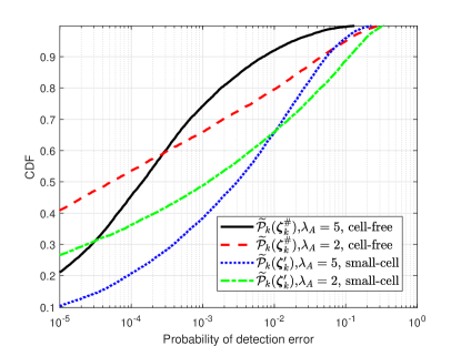
Fig. 6 plots the CDF of the detection error probability 𝒫~k(𝜻k#)\widetilde{{\mathcal{P}}}_{k}({\boldsymbol{\zeta}}^{\#}_{k}) for 2000 realizations of large-scale fading coefficients {βm,k}\{\beta_{m,k}\}. For cell-free IoT networks, it is interesting to investigate the impact of density of APs. To do this, we fix NλA=10N\lambda_{A}=10, which implies the average total number of antennas in an unit area is fixed, and use λA=2\lambda_{A}=2 and 5. By adopting the fusing weight 𝜻k#{\boldsymbol{\zeta}}^{\#}_{k}, the detection error probabilities can be significantly reduced compared with fusing weights 𝜻k{\boldsymbol{\zeta}}^{\prime}_{k}. We also note that the 95%\% likely performance of 𝒫~k(𝜻k#)\widetilde{{\mathcal{P}}}_{k}({\boldsymbol{\zeta}}^{\#}_{k}) with λA=5\lambda_{A}=5 is 2 %\%, while the 95%\% likely performance of 𝒫~k(𝜻k#)\widetilde{{\mathcal{P}}}_{k}({\boldsymbol{\zeta}}^{\#}_{k}) with λA=2\lambda_{A}=2 is 10 %\%. Therefore, larger density of APs allows to improve the accuracy of activity detection when giving the total number of antennas. This observation is expected since the larger number of APs, the higher chances that some of them are located close to an active user.

Refer to caption
Figure 5: The average detection error probability versus the determining radius R1R_{1}
Refer to caption
Figure 6: The CDF of detection error probability with fixed NλA=10N\lambda_{A}=10

Finally, we compare the coverage probability of three systems, namely cell-free IoT, collocated massive MIMO, and small-cell IoT for 2,0002,000 realizations of path-loss coefficients {βl,k}\{\beta_{l,k}\}. Fig. 7 shows the coverage probabilities with P0=0.02P_{0}=0.02 versus the number of antennas NN at each AP. With the increase of NN, all the coverage probability increase significantly. The figure reveals that the closed-form expressions for the small cell system and the collocated massive MIMO match well with the simulation results by averaging over 2,0002,000 realizations of path-loss coefficients. The coverage probability of cell-free networks with 𝜻k#{\boldsymbol{\zeta}}_{k}^{\#} is much higher than the coverage probabilities of small-cell systems and co-located MIMO.

Refer to caption
Figure 7: The coverage probability versus the number of antenna at each AP NN

VII Conclusion

We investigated the activity detection and channel estimation for a cell-free IoT network with massive random access. Focusing on the distributed and user-centric architecture, we proposed a two-stage approach based on the vector AMP algorithm. We derived the activity detection error probability and the mean-squared channel estimation error in closed-form as metrics for a typical device. We defined the coverage probability as a performance metric for the stochastic network. Numerical results show that the coverage probability of the cell-free IoT network can be significantly improved compared with the collocated massive MIMO and small-cell counterparts.

Appendices

VII-A Useful Lemmas

Lemma 3

Let 𝐀τ×τ{\boldsymbol{A}}\in\mathbb{C}^{\tau\times\tau} be a Hermitian invertible matrix. Then, for any vector 𝐱τ{\boldsymbol{x}}\in\mathbb{C}^{\tau} and any scalar aa\in\mathbb{C} such that 𝐀+a𝐱𝐱H{\boldsymbol{A}}+a{\boldsymbol{x}}{\boldsymbol{x}}^{H} is invertible, we have

𝒙H(𝑨+a𝒙𝒙H)1=𝒙H𝑨11+a𝒙H𝑨1𝒙,\displaystyle{\boldsymbol{x}}^{H}\left({\boldsymbol{A}}+a{\boldsymbol{x}}{\boldsymbol{x}}^{H}\right)^{-1}=\frac{{\boldsymbol{x}}^{H}{\boldsymbol{A}}^{-1}}{1+a{\boldsymbol{x}}^{H}{\boldsymbol{A}}^{-1}{\boldsymbol{x}}}, (81)
(𝑨+a𝒙𝒙H)1𝒙=𝑨1𝒙1+a𝒙H𝑨1𝒙.\displaystyle\left({\boldsymbol{A}}+a{\boldsymbol{x}}{\boldsymbol{x}}^{H}\right)^{-1}{\boldsymbol{x}}=\frac{{\boldsymbol{A}}^{-1}{\boldsymbol{x}}}{1+a{\boldsymbol{x}}^{H}{\boldsymbol{A}}^{-1}{\boldsymbol{x}}}. (82)
Lemma 4

Let 𝐀τ×τ{\boldsymbol{A}}\in\mathbb{C}^{\tau\times\tau}, and 𝐱,𝐲𝒞𝒩(𝟎,1τ𝐈τ){\boldsymbol{x}},{\boldsymbol{y}}\sim\mathcal{CN}({\boldsymbol{0}},\frac{1}{\tau}{\boldsymbol{I}}_{\tau}). Assume that 𝐀{\boldsymbol{A}} has uniformly bounded spectral norm (with respect to τ\tau) and that 𝐱{\boldsymbol{x}} and 𝐲{\boldsymbol{y}} are mutually independent and independent of 𝐀{\boldsymbol{A}}, we have

𝒙H𝑨𝒙tr𝑨/ττa.s.0,\displaystyle{\boldsymbol{x}}^{H}{\boldsymbol{A}}{\boldsymbol{x}}-{{\rm tr}{\boldsymbol{A}}}/{\tau}\mathop{-\!\!\!\!-\!\!\!\!-\!\!\!\!-\!\!\!\!-\!\!\!\!-\!\!\!\!\longrightarrow}\limits_{\tau\rightarrow\infty}^{{\rm a}.{\rm s}.}0, (83)
𝒙H𝑨𝒚τa.s.0.\displaystyle{\boldsymbol{x}}^{H}{\boldsymbol{A}}{\boldsymbol{y}}\mathop{-\!\!\!\!-\!\!\!\!-\!\!\!\!-\!\!\!\!-\!\!\!\!-\!\!\!\!\longrightarrow}\limits_{\tau\rightarrow\infty}^{{\rm a}.{\rm s}.}0. (84)
Lemma 5

Let 𝐱,𝐲N{\boldsymbol{x}},~{}{\boldsymbol{y}}\in\mathbb{C}^{N} be two independent random variables satisfying p𝐗(𝐱)=p𝐗(𝐱)p_{\boldsymbol{X}}({\boldsymbol{x}})=p_{\boldsymbol{X}}(-{\boldsymbol{x}}) and p𝐘(𝐲)=p𝐘(𝐲)p_{\boldsymbol{Y}}({\boldsymbol{y}})=p_{\boldsymbol{Y}}(-{\boldsymbol{y}}), and f(𝐱,𝐲)f({\boldsymbol{x}},{\boldsymbol{y}}) be an even function. Then we have

𝔼𝒙,𝒚[f(𝒙,𝒚)𝒙H𝒚]=0.\displaystyle\mathbb{E}_{{\boldsymbol{x}},~{}{\boldsymbol{y}}}[f({\boldsymbol{x}},~{}{\boldsymbol{y}}){\boldsymbol{x}}^{H}{\boldsymbol{y}}]=0. (85)
Lemma 6

Let x,yx,~{}y\in\mathbb{C} are two i.i.d. random variables, and f(x,y)f(x,y) is a symmetric function satisfying

f(x=x0,y=y0)=f(x=y0,y=x0),f(x=x_{0},y=y_{0})=f(x=y_{0},y=x_{0}),

for any x0,y0x_{0},~{}y_{0}\in\mathbb{C}, we have

𝔼x,y[f(x,y)xHx]=𝔼x,y[f(x,y)yHy].\displaystyle\mathbb{E}_{x,y}[f(x,y)x^{H}x]=\mathbb{E}_{x,y}[f(x,y)y^{H}y]. (86)
Lemma 7 (Properties of Gamma Functions[22])
  1. 1.

    As (s)>0\Re(s)>0, we have

    γ(s,x)+Γ(s,x)=Γ(s).\displaystyle{\gamma}(s,x)+{\Gamma}(s,x)={\Gamma}(s). (87)
  2. 2.

    As s{\displaystyle s\to\infty} and nn\in\mathbb{C}, we have the following asymptotic approximation

    limsΓ(s+n)Γ(s)sn=1.\displaystyle\mathop{\lim}_{s\rightarrow\infty}\frac{\Gamma(s+n)}{\Gamma(s)s^{n}}=1. (88)
  3. 3.

    As s{\displaystyle s\to\infty}, we have the following asymptotic approximation

    limsΓ(s+1)=2πssses.\displaystyle\mathop{\lim}_{s\rightarrow\infty}\Gamma(s+1)=\sqrt{2\pi s}s^{s}e^{-s}. (89)
  4. 4.

    As (s)>0\Re(s)>0, the power series expansion of the lower incomplete gamma function is

    γ(s,x)=xsexΓ(s)i=0xiΓ(s+i+1).\displaystyle{\gamma}(s,x)=x^{s}e^{-x}\Gamma(s)\sum\nolimits_{i=0}^{\infty}\frac{x^{i}}{\Gamma(s+i+1)}. (90)
  5. 5.

    As s/(xs)0{\sqrt{s}}/{(x-s)}\rightarrow 0, the asymptotic expansion of the upper incomplete gamma function is given by [23, 24, 25]

    Γ(s,x)\displaystyle\Gamma(s,x) =exxsxs+1{1s1(xs+1)2\displaystyle=\frac{e^{-x}x^{s}}{x-s+1}\left\{1-\frac{s-1}{(x-s+1)^{2}}\right.
    +2(s1)(xs+1)3+O((s1)2(xs+1)4)}.\displaystyle\left.+\frac{2(s-1)}{(x-s+1)^{3}}+O\left(\frac{(s-1)^{2}}{(x-s+1)^{4}}\right)\right\}. (91)

VII-B Proof of Theorem 1

Since 𝒙m,kp𝒙m,k=(1ϵ)δ𝟎+ϵp𝒈m,k{\boldsymbol{x}}_{m,k}\sim p_{{\boldsymbol{x}}_{m,k}}=(1-\epsilon)\delta_{\bf 0}+\epsilon p_{{\boldsymbol{g}}_{m,k}}, where p𝒈m,kp_{{\boldsymbol{g}}_{m,k}} is the PDF of 𝒈m,k𝒞𝒩(𝟎,βm,k𝑰N){\boldsymbol{g}}_{m,k}\sim\mathcal{CN}({\boldsymbol{0}},{\beta}_{m,k}{\boldsymbol{I}}_{N}), the initial state 𝚯m,(0){\boldsymbol{\Theta}}_{m,(0)} in (12) can be simplified into

𝚯m,(0)=θ(m,0)𝑰N,\displaystyle{\boldsymbol{\Theta}}_{m,(0)}=\theta_{(m,0)}{\boldsymbol{I}}_{N}, (92)

where θm,(0)\theta_{m,(0)} is given in (15a).

𝚯m,(t+1)\displaystyle\boldsymbol{\Theta}_{m,(t+1)} =𝑰E+|𝒟m|τ𝔼𝒟m{[η(𝑿^m,k,(t))𝑿m,k][η(𝑿^m,k,(t))𝑿m,k]H}\displaystyle=\frac{\boldsymbol{I}}{E}+\frac{|\mathcal{D}_{m}|}{\tau}\mathbb{E}_{\mathcal{D}_{m}}\left\{[\eta(\widehat{\boldsymbol{X}}_{m,k,(t)})-{\boldsymbol{X}}_{m,k}][\eta(\widehat{\boldsymbol{X}}_{m,k,(t)})-{\boldsymbol{X}}_{m,k}]^{H}\right\}
=(a)𝑰E+|𝒟m|τ𝔼𝒟m{[ξm,k,(t)𝑿^m,k,(t)𝑿m,k][ξm,k,(t)𝑿^m,k,(t)𝑿m,k]H}\displaystyle\overset{(a)}{=}\frac{\boldsymbol{I}}{E}+\frac{|\mathcal{D}_{m}|}{\tau}\mathbb{E}_{\mathcal{D}_{m}}\left\{\left[\xi_{m,k,(t)}\widehat{{\boldsymbol{X}}}_{m,k,(t)}-{\boldsymbol{X}}_{m,k}\right]\left[\xi_{m,k,(t)}\widehat{{\boldsymbol{X}}}_{m,k,(t)}-{\boldsymbol{X}}_{m,k}\right]^{H}\right\}
=(b)𝑰E+|𝒟m|τ𝔼𝒟m{(ξm,k,(t)1)2𝑿m,k𝑿m,kH+(ξm,k,(t)θ(t))2𝑽m,k𝑽m,kH\displaystyle\overset{(b)}{=}\frac{\boldsymbol{I}}{E}+\frac{|\mathcal{D}_{m}|}{\tau}\mathbb{E}_{\mathcal{D}_{m}}\left\{\left(\xi_{m,k,(t)}-1\right)^{2}{{\boldsymbol{X}}}_{m,k}{{\boldsymbol{X}}}_{m,k}^{H}+\left(\xi_{m,k,(t)}\theta_{(t)}\right)^{2}{{\boldsymbol{V}}_{m,k}}{{\boldsymbol{V}}}_{m,k}^{H}\right.
+(ξm,k,(t)1)ξm,k,(t)θ(t)(𝑿m,k𝑽m,kH+𝑽m,k𝑿m,kH)}\displaystyle\left.\qquad\qquad\quad+\left(\xi_{m,k,(t)}-1\right)\xi_{m,k,(t)}\theta_{(t)}\left({{\boldsymbol{X}}}_{m,k}{{\boldsymbol{V}}}_{m,k}^{H}+{{\boldsymbol{V}}}_{m,k}{{\boldsymbol{X}}}_{m,k}^{H}\right)\right\}
=(c)𝑰E+|𝒟m|τ𝔼𝒟m{(ξm,k,(t)1)2𝑿m,k𝑿m,kH+(ξm,k,(t)θ(t))2𝑽m,k𝑽m,kH},\displaystyle\overset{(c)}{=}\frac{\boldsymbol{I}}{E}+\frac{|\mathcal{D}_{m}|}{\tau}\mathbb{E}_{\mathcal{D}_{m}}\left\{\left(\xi_{m,k,(t)}-1\right)^{2}{{\boldsymbol{X}}}_{m,k}{{\boldsymbol{X}}}_{m,k}^{H}+\left(\xi_{m,k,(t)}\theta_{(t)}\right)^{2}{{\boldsymbol{V}}_{m,k}}{{\boldsymbol{V}}}_{m,k}^{H}\right\}, (93)

For given 𝚯(t)=θm,(t)𝑰N{\boldsymbol{\Theta}}_{(t)}=\theta_{m,(t)}{\boldsymbol{I}}_{N}, using (III-A), we have (VII-B) shown at the top of this page. Step (a) is obtained according the definition of MMSE denoiser given in (14) and assumption 𝚯m,(t)=θm,(t)𝑰N{\boldsymbol{\Theta}}_{m,(t)}=\theta_{m,(t)}{\boldsymbol{I}}_{N}, step (b) is obtained according to the signal model (11), step (c) is obtained using Lemma 5 since ξm,k,(t)\xi_{m,k,(t)} is an even function w.r.t. 𝑿m,k{\boldsymbol{X}}_{m,k} and 𝑽m,k{\boldsymbol{V}}_{m,k} according to (13c), (12a)-(12c), and (9).

Define

𝑩\displaystyle{\boldsymbol{B}} =𝔼𝒟m[(ξm,k,(t)1)2𝑿m,k𝑿m,kH\displaystyle=\mathbb{E}_{\mathcal{D}_{m}}\left[\left(\xi_{m,k,(t)}-1\right)^{2}{{\boldsymbol{X}}}_{m,k}{{\boldsymbol{X}}}_{m,k}^{H}\right.
+ξm,k,(t)2θm,(t)2𝑽m,k𝑽m,kH].\displaystyle\qquad\qquad\qquad\left.+\xi_{m,k,(t)}^{2}\theta_{m,(t)}^{2}{{\boldsymbol{V}}_{m,k}}{{\boldsymbol{V}}}_{m,k}^{H}\right]. (94)

For the non-diagonal entity 𝑩(i,j){\boldsymbol{B}}_{(i,j)} with iji\neq j, we have

𝑩(i,j)\displaystyle{\boldsymbol{B}}_{(i,j)} =𝔼𝒟m[(ξm,k,(t)1)2[𝑿m,k](i)[𝑿m,k](j)\displaystyle=\mathbb{E}_{\mathcal{D}_{m}}\left[\left(\xi_{m,k,(t)}-1\right)^{2}\left[{{\boldsymbol{X}}}_{m,k}\right]_{(i)}\left[{{\boldsymbol{X}}}_{m,k}^{*}\right]_{(j)}\right.
+ξm,k,(t)2θm,(t)2[𝑽m,k](i)[𝑽m,k](j)]=0\displaystyle\left.+\xi_{m,k,(t)}^{2}\theta_{m,(t)}^{2}\left[{{\boldsymbol{V}}_{m,k}}\right]_{(i)}\left[{{\boldsymbol{V}}}_{m,k}^{*}\right]_{(j)}\right]=0 (95)

where the last step follows from Lemma 5 since [𝑿m,k](i)\left[{\boldsymbol{X}}_{m,k}\right]_{(i)} and [𝑽m,k](i)\left[{\boldsymbol{V}}_{m,k}\right]_{(i)} are independent of [𝑿m,k](j)\left[{\boldsymbol{X}}_{m,k}\right]_{(j)} and [𝑽m,k](j)\left[{\boldsymbol{V}}_{m,k}\right]_{(j)}, respectively. For the diagonal entities, according to Lemma 6, we have

[𝑩](i,i)=[𝑩](j,j),i,j=1,,N,\left[{\boldsymbol{B}}\right]_{(i,i)}=\left[{\boldsymbol{B}}\right]_{(j,j)},~{}\forall i,j=1,\cdots,N,

since ξm,k,(t)\xi_{m,k,(t)} is a symmetric function of the entities of 𝑿m,k{\boldsymbol{X}}_{m,k} and 𝑽m,k{\boldsymbol{V}}_{m,k}. Hence, we have

[𝑩](i,i)=tr[𝑩]N,i=1,,N.\displaystyle\left[{\boldsymbol{B}}\right]_{(i,i)}=\frac{{\rm tr}[{\boldsymbol{B}}]}{N},~{}\forall i=1,\cdots,N. (96)

According to (VII-B) and (96), 𝚯m,(t+1)\boldsymbol{\Theta}_{m,(t+1)} can be further simplified as

𝚯m,(t+1)=θm,(t+1)𝑰N,\displaystyle{\boldsymbol{\Theta}}_{m,(t+1)}=\theta_{m,(t+1)}{\boldsymbol{I}}_{N}, (97)

with θm,(t+1)\theta_{m,(t+1)} defined in (15b). Combining (92) and (97), we complete the proof.

VII-C Proof of Lemma 1

For c(0,1)c\in(0,1), we have

lims+γ(s,cs)Γ(s)=(90)\displaystyle\mathop{\lim}_{s\rightarrow+\infty}\frac{{\gamma}(s,cs)}{\Gamma(s)}\overset{(\ref{Gamma_pro4})}{=} lims+(cs)se(cs)i=0(cs)iΓ(s+i+1)\displaystyle\mathop{\lim}_{s\rightarrow+\infty}\frac{(cs)^{s}}{e^{(cs)}}\sum_{i=0}^{\infty}\frac{(cs)^{i}}{\Gamma(s+i+1)}
(88)\displaystyle\overset{(\ref{Gamma_pro2})}{\geq} lims+(cs)se(cs)i=0(cs)iΓ(s)(s)i+1\displaystyle\mathop{\lim}_{s\rightarrow+\infty}\frac{(cs)^{s}}{e^{(cs)}}\sum_{i=0}^{\infty}\frac{(cs)^{i}}{\Gamma(s)(s)^{i+1}}
=\displaystyle= lims+(cs)ssΓ(s)e(cs)i=0(c)i\displaystyle\mathop{\lim}_{s\rightarrow+\infty}\frac{(cs)^{s}}{s\Gamma(s)e^{(cs)}}\sum_{i=0}^{\infty}(c)^{i}
=\displaystyle= lims+(cs)se(cs)s(1c)Γ(s)\displaystyle\mathop{\lim}_{s\rightarrow+\infty}\frac{(cs)^{s}e^{(-cs)}}{s(1-c)\Gamma(s)}
=(88)\displaystyle\overset{(\ref{Gamma_pro2})}{=} lims+(cs)se(cs)(1c)Γ(s+1)\displaystyle\mathop{\lim}_{s\rightarrow+\infty}\frac{(cs)^{s}e^{(-cs)}}{(1-c)\Gamma(s+1)}
=(89)\displaystyle\overset{(\ref{Gamma_pro3})}{=} lims+(cs)ses2πsss(1c)e(cs)\displaystyle\mathop{\lim}_{s\rightarrow+\infty}\frac{(cs)^{s}e^{s}}{\sqrt{2\pi s}s^{s}(1-c)e^{(cs)}}
=\displaystyle= lims+1(1c)2πs(ceec)s\displaystyle\mathop{\lim}_{s\rightarrow+\infty}\frac{1}{(1-c)\sqrt{2\pi s}}\left(\frac{ce}{e^{c}}\right)^{s}
=\displaystyle= 0,\displaystyle 0, (98)

where the last step is based on the fact

0<ceec<1,as0c1.0<\frac{ce}{e^{c}}<1,~{}\mbox{as}~{}0\leq c\leq 1.

Consider now the case c>1c^{\prime}>1. By substituting x=csx=c^{\prime}s into (5) and taking the limit, we obtain

lims+Γ(s,cs)Γ(s)=\displaystyle\mathop{\lim}_{s\rightarrow+\infty}\frac{{\Gamma}(s,c^{\prime}s)}{\Gamma(s)}= lims+(cs)se(cs)(c1)sΓ(s)\displaystyle\mathop{\lim}_{s\rightarrow+\infty}\frac{(c^{\prime}s)^{s}e^{(-c^{\prime}s)}}{(c^{\prime}-1)s\Gamma(s)} (99)
=(88)\displaystyle\overset{(\ref{Gamma_pro2})}{=} lims+(cs)se(cs)(c1)Γ(s+1)\displaystyle\mathop{\lim}_{s\rightarrow+\infty}\frac{(c^{\prime}s)^{s}e^{(-c^{\prime}s)}}{(c^{\prime}-1)\Gamma(s+1)} (100)
=(89)\displaystyle\overset{(\ref{Gamma_pro3})}{=} lims+(cs)se(cs)es(c1)2πsss\displaystyle\mathop{\lim}_{s\rightarrow+\infty}\frac{(c^{\prime}s)^{s}e^{(-c^{\prime}s)}e^{s}}{(c^{\prime}-1)\sqrt{2\pi s}s^{s}} (101)
=\displaystyle= lims+1(c1)2πs(ceec)s\displaystyle\mathop{\lim}_{s\rightarrow+\infty}\frac{1}{(c^{\prime}-1)\sqrt{2\pi s}}\left(\frac{c^{\prime}e}{e^{c^{\prime}}}\right)^{s} (102)
=\displaystyle= 0,\displaystyle 0, (103)

where the last equality is based on the fact

0<ceec<1,asc>1.0<\frac{ce}{e^{c}}<1,~{}\mbox{as}~{}c>1.

References

  • [1] A. Al-Fuqaha, M. Guizani, M. Mohammadi, M. Aledhari, and M. Ayyash, “Internet of things: A survey on enabling technologies, protocols, and applications,” IEEE Commun. Surveys & Tuts., vol. 17, no. 4, pp. 2347–2376, Fourthquarter 2015.
  • [2] S. Mumtaz, A. Alsohaily, Z. Pang, A. Rayes, K. F. Tsang, and J. Rodriguez, “Massive internet of things for industrial applications: addressing wireless IIoT connectivity challenges and ecosystem fragmentation,” IEEE Ind. Electron. Mag., vol. 11, no. 1, pp. 28–33, 2017.
  • [3] K. Senel and E. G. Larsson, “Device activity and embedded information bit detection using AMP in massive MIMO,” IEEE Globecom Workshops (GC Wkshps), Singapore, 2017, pp. 1–6.
  • [4] M. Hasan, E. Hossain, and D. Niyato, “Random access for machine-to-machine communication in LTE-advanced networks: issues and approaches,” IEEE Commun. Mag., vol. 51, no. 6, pp. 86–93, Jun. 2013.
  • [5] D. Zhai, R. Zhang, L. Cai, B. Li, and Y. Jiang, “Energy-efficient user scheduling and power allocation for NOMA based wireless networks with massive IoT devices,” IEEE Internet Things J., vol. 5, no. 3, pp. 1857–1868, Jun. 2018.
  • [6] L. Liu, E. G. Larsson, W. Yu, P. Popovski, C. Stefanovic, and E. de Carvalho, “Sparse signal processing for grant-free massive connectivity: A future paradigm for random access protocols in the Internet of Things,” IEEE Signal Process. Mag., vol. 35, no. 5, pp. 88–99, Sep. 2018.
  • [7] H. Zhu and G. B. Giannakis, “Exploiting sparse user activity in multi-user detection,” IEEE Trans. Commun., vol. 59, no. 2, pp. 454–465, Feb. 2011.
  • [8] Z. Chen and W. Yu, “Massive device activity detection by approximate message passing,” in Proc. IEEE Int. Conf. Acoust., Speech, Signal Process., pp. 3514–3518, Mar. 2017.
  • [9] Z. Chen, F. Sohrabi, and W. Yu, “Sparse activity detection for massive connectivity,” IEEE Trans. Signal Process., vol. 66, no. 7, pp. 1890–1904, Apr. 2018
  • [10] L. Liu and W. Yu, “Massive connectivity with massive MIMO—Part I: Device activity detection and channel estimation,” IEEE Trans. Signal Process., 2018, vol. 66, no. 11, pp. 2933–2946, 2018.
  • [11] H. Q. Ngo, A. Ashikhmin, H. Yang, E. G. Larsson, and T. L. Marzetta, “Cell-free massive MIMO versus small cells,” IEEE Trans. on Wireless Commun., vol. 16, no. 3, pp. 1834–1850, Mar. 2017.
  • [12] J. Zhang, S. Chen, Y. Lin, J. Zheng, B. Ai, and L. Hanzo, “Cell-free massive MIMO: A new next-generation paradigm,” IEEE Access, vol. 7, pp. 99878–99888, 2019.
  • [13] S. Buzzi, C. D’Andrea, A. Zappone, and C. D’Elia, “User-centric 5G cellular networks: Resource allocation and comparison with the cell-free massive MIMO approach,” IEEE Trans. Wireless Commun., vol. 19, no. 2, pp. 1250–1264, Feb. 2020.
  • [14] S. Rao, A. Ashikhmin, and H. Yang “Internet of things based on cell-free massive MIMO,” in Proc. 53rd Asilomar Conf. Signals, Syst. Comput., 2019, pp. 1946–1950.
  • [15] X. Wang, A. Ashikhmin, and Xiaodong Wang, “Wirelessly powered cell-free IoT: analysis and optimization,” IEEE Internet Things J., vol. 7, no. 9, pp. 8384–8396, Sep. 2020.
  • [16] A.-S. Bana, E. de Carvalho, B. Soret, T. Abrao, J. C. Marinello, E. G. Larsson, and P. Popovski, “Massive MIMO for Internet of things (IoT) connectivity,” arXiv:1905.06205, May 2019.
  • [17] J. Hoydis, S. ten Brink, and M. Debbah, “Massive MIMO in the UL/DL of cellular networks: how many antennas do we deed?,” IEEE J. Sel. Areas Commun., vol. 31, no. 2, pp. 160–171, Feb. 2013.
  • [18] X. Shao, X. Chen, C. Zhong, J. Zhao, and Z. Zhang, “A unified design of massive access for cellular internet of things,” IEEE Internet Things J., vol. 6, no. 2, pp. 3934–3947, Apr. 2019.
  • [19] J. Jose, A. Ashikhmin, T. L. Marzetta, and S. Vishwanath, “Pilot contamination and precoding in multi-cell TDD systems,” IEEE Trans. Wireless Commun., vol. 10, no. 8, pp. 2640–2651, Aug. 2011.
  • [20] F. E. Satterthwaite, “An approximate distribution of estimates of variance components,” Biometrics Bull., vol. 2, no. 6, pp. 110–114, Dec. 1946.
  • [21] B. L. Welch, “The generalization of ‘Student’s’ problem when several different population variances are involved,” Biometrika, vol. 34, nos. 1-2, pp. 28–35, Jan. 1947.
  • [22] Abramowitz, M. and Stegun, I. A. “Handbook of Mathematical Functions with Formulas, Graphs, and Mathematical Tables”, 9th printing. New York: Dover, 1972.
  • [23] F. G. Tricomi, “Asymptotische eigenschaften der unvollstandigen gammafunktion,” Math. Z., vol. 53, pp. 136–148, 1950.
  • [24] W. Gautschi, “The incomplete gamma functions since Tricomi,” Atti dei Convegni Linci, no. 147, pp. 203–237, 1998.
  • [25] M. Sharif and B. Hassibi, “A comparison of time-sharing, DPC, and beamforming for MIMO broadcast channels with many users,” IEEE Trans. Commun., vol. 55, no. 1, pp. 11–15, Jan. 2007.