Two distinct types of echoes in compact objects

The inception of gravitational wave (GW) observation, facilitated by direct waveform captures [1, 2, 3, 4], has initiated a groundbreaking phase in observational astronomy. This novel research domain is dedicated to exploring the strong-field gravity sector, which has experienced rapid progress lately. Notably, current endeavors in space-based laser interferometry [5, 6, 7] have led to significant advancements aimed at achieving unmatched detector sensitivity [8, 9, 10, 11, 12].

Theoretical insights have been instrumental in assessing the feasibility of black hole spectroscopy [13, 14, 15, 16, 17, 18]. Specifically, in the context of real-world phenomena, sources of gravitational radiation such as black holes and neutron stars are embedded within a medium, not existing in isolation. This consideration inevitably alters spacetime from a perfect symmetric metric, substantially modifying the GWs emitted from such an entity. Such observations have directed research focus towards “dirty” black holes [19, 20, 21, 22], thus broadening the scope of black hole perturbation theory.

Within this framework, there has been a concentrated effort on constructing realistic models involving compact astrophysical bodies, including binaries of black holes or neutron stars. The investigation of black hole quasinormal modes (QNMs) [23, 24, 25] has been a primary focus, given their critical role during the ringdown phase post-merger. These modes, which are dissipative oscillations reflective of the core characteristics of the black hole spacetime, adhere to several no-hair theorems [26, 27]. Initial studies by Leung et al. [20] on scalar QNMs of non-rotating “dirty” black holes, evaluating shifts in quasinormal frequencies through generalized logarithmic perturbation theory, laid the groundwork in this area. Further analysis by Barausse et al. on perturbations surrounding a central Schwarzschild black hole [22] demonstrated that the resulting QNMs could exhibit significant deviations from an isolated black hole’s characteristics. Nevertheless, they posited that the influence of the astrophysical environment on black hole spectroscopy could be minimal if appropriate waveform templates were applied. Among the scenarios examined in [22], the thin shell model was identified as having a significant effect on the QNM spectrum. The concept of the black hole pseudospectrum, introduced by Nollert and Price [28, 29], aligns with these insights, showing how minimal perturbations, depicted as step functions, could remarkably influence high-overtone QNM modes, thus revealing a sizable susceptibility of the QNM spectrum to “ultraviolet” perturbations. Our prior work [30] contended that discontinuities could alter the QNM spectrum’s asymptotic behavior non-perturbatively, causing high-overtone modes to transition along the real axis rather than the imaginary frequency axis [31, 32], a phenomenon observed irrespective of the discontinuity’s proximity to the horizon or its order. Through the notion of structural stability, Jaramillo et al. [33, 34, 35] explored the effects of metric randomizations, with their findings via the hyperboloidal coordinates [36] indicating a shift of the pseudospectrum’s boundary towards the real frequency axis, thereby emphasizing the inherent instability of high-overtone modes to ultraviolet perturbations. Recent findings by Cheung et al. [37] also suggest the vulnerability of even the fundamental mode to destabilization by generic perturbations.

Cardoso et al. introduced the concept of echoes [38], a novel phenomenon intersecting with late-stage ringing waveforms, potentially distinguishing different gravitational systems through unique near-horizon characteristics. This concept has spurred numerous investigations [39, 40, 41] into echoes across various systems, including exotic compact objects such as gravastars [42, 43], wormholes [44, 45, 46, 47, 48, 49, 50], among others.

On the analytic aspect, echoes’ derivation from Green’s function’s properties, especially its asymptotic behavior, was furthered by Mark et al. [51] through frequency domain evaluation. Echo phenomena in compact objects were then conceptualized by reinterpreting the response waveform as a series summation of reflection and transmission amplitudes alongside the convolution integration process in the inverse Fourier transform. From the viewpoint of a scattering process, investigations of echoes within the framework of Damour-Solodukhin type wormholes [48] by Bueno et al. [52] involved solving for specific frequencies at which the transition matrix turns singular, leading to identifiable quasinormal frequencies that give rise to echoes. While most scenarios of echoes occur for effective potentials possessing two local maxima, some of us proposed an alternative mechanism for echoes [53] without necessarily introducing a second local maximum in the effective potential. The Green’s function’s approach was adapted, and the echoes’ emergence is linked to the asymptotic pole structure of the QNM spectrum [30, 54] due to some minor discontinuity planted into the potential. This suggests that discontinuity might serve an alternative ingredient for echo mechanism.

In principle, it can be argued that both approaches stand on an equivalent theoretical foundation concerning a peculiar property of the transit amplitudes. However, from a physical perspective, they can be viewed as two distinct mechanisms for generating echoes. In the first scenario, the effective potential is characterized by two local maxima separated by a distance, creating a potential well [52, 55], with Damour-Solodukhin type wormholes [52] serving as a prime example. Echoes in this context can be intuitively understood as resulting from repeated reflections of GWs within such a potential well, with the echo period mathematically determined as twice the distance between the maxima of the effective potential via the spatial displacement operator that separates the two local maxima. The second scenario entails a degree of discontinuity within the effective potential [51, 53], potentially brought about by specific accretion processes giving rise to “cuspy” [56, 57, 58] or “splashback” [59, 60] profiles, without necessarily leading to a second local maximum in the effective potential. This gives rise to echo signals typically attenuated over time, with their period dictated by the characteristics of the relevant transfer amplitudes. For both cases, the echoes correspond to a novel category of quasinormal modes with minor real parts, and the echo period is associated with the spacing, along the direction of the real frequency axis, between successive modes [53].

The present study aims to explore this topic further, proposing a unified model within compact stars that encompasses both echo mechanisms. We demonstrate that the two types of echoes, stemming from distinct physical origins, can be independently triggered within such a model, as evidenced through numerical simulations. The remainder of the work is structured as follows. In Sec. II, we delve into Green’s function approach for the two distinct echo mechanisms. Subsequently, in Sec. III, we provide an overview of axial gravitational perturbations in compact stars, serving as a comprehensive theoretical setup for the emergence of echoes through both mechanisms. The master equation for the perturbations is formulated for compact stars of uniform density. Numerical results are presented in Sec. IV, where spatial-temporal evolutions are calculated using the finite difference method, elucidating the principal characteristics of the echoes and the interplay between the two mechanisms. Additional discussions and concluding remarks are given in Sec. V.

This section explores Green’s function formalism within black hole perturbation theory and its application to echoes in compact objects. When variable separation is achievable, the evolution of perturbations simplifies, with the dynamics predominantly governed by the radial component of the master equation [24, 25]:

$\displaystyle\frac{\partial^{2}}{\partial t^{2}}\Psi(t,x)+\left(-\frac{\partial^{2}}{\partial x^{2}}+V_{\mathrm{eff}}\right)\Psi(t,x)=0,$

(1)

where $x$ denotes the tortoise coordinate, and $V_{\mathrm{eff}}$ represents the effective potential defined by the spacetime metric, spin ${\bar{s}}$, and angular momentum $\ell$ of the waveform. For example, the Regge-Wheeler potential $V_{\mathrm{RW}}$ for a Schwarzschild black hole metric is given by

$\displaystyle V_{\mathrm{eff}}=V_{\mathrm{RW}}=F\left[\frac{\ell(\ell+1)}{r^{2}}+(1-{\bar{s}}^{2})\frac{r_{h}}{r^{3}}\right],$

(2)

where

$\displaystyle F=1-r_{h}/r,$

(3)

$r_{h}=2M$ represents the horizon, with $M$ being the black hole mass, and the tortoise coordinate relates to the radial coordinate $r$ through $x=\int dr/F(r)$.

QNMs of black holes are determined by solving the eigenvalue problem presented in Eq. (1) in the frequency domain:

$$\frac{d^{2}\Psi(\omega,x)}{dx^{2}}+[\omega_{n}^{2}-V_{\mathrm{eff}}(r)]\Psi(\omega,x)=0.$$

(4)

For asymptotically flat spacetimes, the boundary conditions are defined as:

$$\Psi\sim\begin{cases}e^{-i\omega_{n}x},&x\to-\infty,\\ e^{+i\omega_{n}x},&x\to+\infty,\end{cases}$$

(5)

indicating an ingoing wave at the horizon and an outgoing wave at infinity, with $n$ denoting the overtone number. Beyond the initial burst, the waveform $\Psi$ is characterized by quasinormal oscillations with complex eigenvalues $\omega_{n}$, termed quasinormal frequencies. The dissipative nature of the system is reflected in the imaginary components of these frequencies.

The QNM properties are intricately linked to the analytic properties of the corresponding Green’s function, satisfying

$$\left[\frac{d^{2}}{dx^{2}}+(\omega_{n}^{2}-V_{\mathrm{eff}}(r))\right]\widetilde{G}(\omega,x,y)=\delta(x-y).$$

(6)

Following established procedures [61, 62, 63], Green’s function is constructed as:

$$\widetilde{G}(\omega,x,y)=\frac{1}{W(\omega)}f(\omega,x_{<})g(\omega,x_{>}),$$

(7)

where $x_{<}\equiv\min(x,y)$, $x_{>}\equiv\max(x,y)$, and

$$W(\omega)\equiv W(g,f)={g}{f}^{\prime}-{f}{g}^{\prime}$$

(8)

is the Wronskian of $f$ and $g$, the two linearly independent solutions of the corresponding homogeneous equation satisfying the boundary conditions Eq. (5) at the horizon and infinity, respectively.

To be specific, $f$ and $g$ demonstrate the following asymptotic behaviors

$$f(\omega,x)\sim\begin{cases}e^{-i\omega x},&x\to-\infty,\\ A_{\mathrm{out}}(\omega)e^{+i\omega x}+A_{\mathrm{in}}(\omega)e^{-i\omega x},&x\to+\infty,\end{cases}$$

(9)

and

$$g(\omega,x)\sim\begin{cases}B_{\mathrm{out}}(\omega)e^{+i\omega x}+B_{\mathrm{in}}(\omega)e^{-i\omega x},&x\to-\infty,\\ e^{+i\omega x},&x\to+\infty,\end{cases}$$

(10)

in spacetimes that are asymptotically flat, remaining bounded as $t\to+\infty$ for $\Im\omega<0$. Herein, $A_{\mathrm{in}}$, $A_{\mathrm{out}}$, $B_{\mathrm{in}}$, and $B_{\mathrm{out}}$ represent the reflection and transmission coefficients, which, although their exact expressions might not be specified in our derivations, are well-defined for a specific metric. These waveform amplitudes adhere to the relations [64]

	$\displaystyle B_{\mathrm{out}}$	$\displaystyle=$	$\displaystyle A_{\mathrm{in}},$
	$\displaystyle B_{\mathrm{in}}$	$\displaystyle=$	$\displaystyle-A_{\mathrm{out}}^{*},$		(11)

as dictated by principles of completeness and conservation of flux. Moreover, the reflection and transmission coefficients for black holes are specified as

	$\displaystyle\widetilde{\mathcal{R}}_{\mathrm{BH}}(\omega)$	$\displaystyle=$	$\displaystyle\frac{B_{\mathrm{in}}}{B_{\mathrm{out}}},$
	$\displaystyle\widetilde{\mathcal{T}}_{\mathrm{BH}}(\omega)$	$\displaystyle=$	$\displaystyle\frac{1}{B_{\mathrm{out}}},$		(12)

for waves originating from $x\to-\infty$.

Echoes, akin to QNMs, are identified by the poles of Green’s function. While the inherent pole structure primarily emerges from the zeros of the Wronskian Eq. (8), it may undergo alterations due to phenomena like pole skipping [65, 66] or additional distortions introduced by an external source [67]. Echoes are categorized within this context. The discussion outlines two scenarios in which particular effective potentials lead to a unique set of poles associated with echoes in compact objects. For the first scenario, the Wronskian is determined by segregating two potential barriers by a specified distance using a spatial displacement operator, interpreting the resultant echoes as repeated GW reflections within a potential well, with the echo period defined by twice the distance separating the two local maxima. The second scenario incorporates discontinuity at a certain order of the effective potential, where the Wronskian is derived from the explicit forms of transmission amplitudes at the discontinuity point. In both instances, it is demonstrated that the resulting mathematical expressions share similarities, and the echoes correspond to a new series of quasinormal modes characterized by minor real parts, with the echo period correlating to the spacing between successive modes in the frequency domain.

The above two types of echoes might be present simultaneously in the context of compact objects. This is because the effective potential of a compact star may possess two local maxima, while the star’s surface usually introduces some discontinuity. In the literature, the well-known w-modes [69, 70, 71, 72] are readily recognized as echoes in star quasinormal modes. However, to our knowledge, an explicit discussion regarding the nuance difference elaborated in the foregoing section has yet to be carried out.

In what follows, we derive the master equation for axial gravitational perturbations in stars of uniform density. To enhance the reader’s understanding, we adopt a minimalist approach that focuses on a spherically symmetric compact star with uniform density, making the physical content more accessible. The spacetime metric possess the form

$\displaystyle ds^{2}=-h(r)dt^{2}+\frac{dr^{2}}{f(r)}+r^{2}\left(d\theta^{2}+\sin^{2}\theta d\varphi^{2}\right).$

(25)

On the outside of the star $r\geq r_{b}$, where $r_{b}$ is the radial coordinate of the star’s surface, the metric is essentially Schwarzschild, which reads

$\displaystyle f(r)=h(r)=1-\frac{2M_{S}}{r},$

(26)

where $M_{S}$ is the mass of the compact object. The tortoise coordinate reads $x\equiv r_{*}=\int dr/\sqrt{fh}=r+r_{S}\log\left(\frac{r}{r_{S}}-1\right)$.

Beneath the surface of a star $r\leq r_{b}$ with uniform density $\rho=\frac{3M_{S}}{4\pi r_{b}^{3}}$, one has [73]

	$\displaystyle f(r)$	$\displaystyle=$	$\displaystyle 1-\frac{2M(r)}{r},$
	$\displaystyle h(r)$	$\displaystyle=$	$\displaystyle\frac{1}{4}\left(3\sqrt{1-\frac{2M(r)}{r}}-\sqrt{1-\frac{2M(r)r^{2}}{r_{b}^{3}}}\right)^{2},$
	$\displaystyle M(r)$	$\displaystyle=$	$\displaystyle\int^{r}_{0}4\pi r^{\prime 2}\rho dr^{\prime}=M_{S}\frac{r^{3}}{r_{b}^{3}},$
	$\displaystyle p(r)$	$\displaystyle=$	$\displaystyle-\rho\left(\frac{\sqrt{1-\frac{2M(r)}{r}}-\sqrt{1-\frac{2M(r)r^{2}}{r_{b}^{3}}}}{3\sqrt{1-\frac{2M(r)}{r}}-\sqrt{1-\frac{2M(r)r^{2}}{r_{b}^{3}}}}\right).$		(27)

For the tortoise coordinate, the constant of integration is chosen so that $x(r=0)=0$.

By using the method of separation of variables, the axial gravitational perturbations are governed by [74]

	$\displaystyle\frac{\partial^{2}\Psi}{\partial r^{2}}-\frac{\partial^{2}\Psi}{\partial t^{2}}-V(r)\Psi=0,$
	$\displaystyle V_{\text{star}}(r)=\frac{h}{r^{3}}\left(\ell(\ell+1)r+4\pi(\rho-p)r^{3}-6M\right),$
	$\displaystyle V_{\text{BH}}(r)=\frac{h}{r^{3}}\left(\ell(\ell+1)r-6M_{S}\right),$		(28)

where $L$ is the angular momentum. At spatial infinity, the boundary condition dictates that the waveform $\Psi$ is an asymptotic outgoing wave. At the star’s center, it must be regular with vanishing flux. Moreover, the junction conditions at the star’s surface reads

	$\displaystyle\Psi_{\text{inside}}(r_{b})$	$\displaystyle=$	$\displaystyle\Psi_{\text{outside}}(r_{b}),$
	$\displaystyle\partial_{r}\Psi_{\text{inside}}(r_{b})$	$\displaystyle=$	$\displaystyle\partial_{r}\Psi_{\text{outside}}(r_{b}),$		(29)

or

$\displaystyle\partial_{x}\Psi_{\text{inside}}(r_{b})=\partial_{x}\Psi_{\text{outside}}(r_{b}).$

(30)

The numerical calculations will be performed using the finite difference method [75, 76, 77]. We will adopt the scheme recently proposed by some of us [78]. In the literature, most implementations are performed in Eddington-Finkelstein coordinates $(u=t-x$, $v=t+x)$, where one implements the initial condition on $v=0$ and the boundary condition on $u=0$, In such circumstances, in the far region where the effective potential asymptotically approaches zero, the initial perturbations will never attain the $u$ axis due to causality constraints. However, in the region where the effective potential does not vanish, there is a chance that the speed of signal propagation exceeds the unit, and initial perturbations placed on the $u$ axis might traverse the $v$ axis. In other words, the boundary condition enforced for $u=0$ might interfere with the initial perturbations’ free propagation.

Conversely, in our proposed scheme, the calculations are implemented in the $(x,t)$ coordinates, and the initial condition is placed on the $t=0$ slice. As a result, the concerns regarding causality will no longer be relevant. In particular, we adopt the initial conditions $\Psi(t=0)$ of a Gaussian form and $\partial_{t}\Psi(t=0)$. One proceeds to discretize the spacetime coordinates and approximates the partial derivatives by first-order finite differences. To be specific, we denote

	$\displaystyle t_{i}$	$\displaystyle=$	$\displaystyle t_{0}+i\Delta t,$
	$\displaystyle x_{j}$	$\displaystyle=$	$\displaystyle x_{0}+j\Delta x$		(31)

and

	$\displaystyle\Psi^{i}_{j}$	$\displaystyle=$	$\displaystyle\Psi(t=t_{i},x=x_{j}),$
	$\displaystyle V_{j}$	$\displaystyle=$	$\displaystyle V(x=x_{j}),$		(32)

and therefore, the master equation Eq. (III) becomes

$\displaystyle\Psi^{i+1}_{j}=-\Psi^{i-1}_{j}+\frac{\Delta t^{2}}{\Delta x^{2}}\left(\Psi^{i}_{j-1}+\Psi^{i-1}_{j}\right)+\left(2-2\frac{\Delta t^{2}}{\Delta x^{2}}-\Delta t^{2}V_{j}\right)\Psi^{i}_{j}.$

(33)

The junction condition Eq. (III) reads

$\displaystyle\frac{\Psi^{i}_{j_{b}}-\Psi^{i}_{j_{b}-1}}{\Delta x}=\frac{\Psi^{i}_{j_{b}+1}-\Psi^{i}_{j_{b}}}{\Delta x},$

(34)

where one uses the subscript $b$ to denote the grid on the star’s surface. Eq. (34) can be simplified to give

$\displaystyle\Psi^{i}_{j_{b}}=\frac{1}{2}\left(\Psi^{i}_{j_{b}+1}+\Psi^{i}_{j_{b}-1}\right),$

(35)

where the subscript $b$ indicates that the grid is on the star’s surface.

As shown in Fig. 1, the numerical iterative process can be performed by using Eqs. (33) and (35). Given the black grids on the boundary, the temporal evolution is implemented by inferring the values of the red grids. For most grids, Eq. (33) is utilized to determine the grid values for the next time step, except for those on the star’s surface. The latter is determined by employing Eq. (35). To avoid the von Neumann instability [79, 80], we choose

$\displaystyle\frac{\Delta t^{2}}{\Delta x^{2}}+\frac{\Delta t^{2}}{4}V_{\text{max}}<1.$

(36)

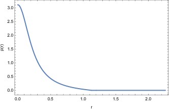
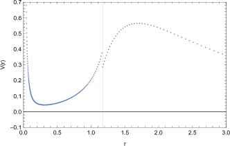
Now, we proceed to present the numerical results. For the first types of echoes, we elaborate two sets of parameters: $M_{S}=\frac{1}{2}$, $r_{b}=1.13$, $\ell=2$, and $M_{S}=\frac{1}{2}$, $r_{b}=1.14$, $\ell=2$. The metric functions are presented in Fig. 2, and the corresponding effective potentials are shown in Fig. 3. When presented in radial coordinate $r$, the forms of the effective potentials are primarily identical, particularly the positions of the two maxima. However, the difference is apparent in terms of the tortoise coordinate $x$. For both parameters, echoes are demonstrated, as shown in Fig. 4. The spatial-temporal evolution indicates that initial perturbations propagate at $v=1$ and are reflected at both maxima. The temporal evolution clearly shows the occurrence of echoes. The distance between the two maxima governs the resulting echoes’ period. Even though a discontinuity is present, it is irrelevant to the observed echoes.

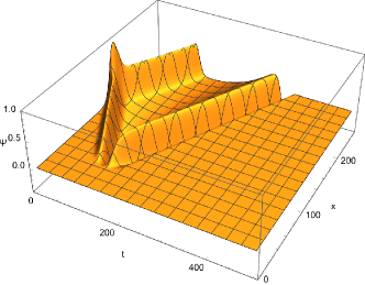
We consider the metric parameters $M_{S}=\frac{1}{2}$, $r_{b}=100$, and $\ell=2$ to demonstrate the second type of echo. As shown in Fig. 5, since the discontinuity is placed beyond the would-be maximum of Regge-Wheeler effective potential, the resulting effective potential does not feature a second maximum. Moreover, the discontinuity is visually insignificant. The resulting echoes are presented in Fig. 6. The echoes’ period is found to be $T\simeq 200$, in accordance with twice the distance between the maximum and the discontinuity of the effective potential. In contrast to Fig. 4, the magnitude of the echoes is suppressed in time. This explains why such echoes were not observed in Fig. 4, as it is likely buried inside the echoes formed by the first type.

Echoes, emerging as a novel observable in the GW spectrum, offer a unique window into the physics of compact objects and their environments. By exploring the nuances of echo mechanisms through a unified model, this study contributes to a deeper understanding of the complex interplay between GWs and the structure of compact objects. Through numerical simulations, we demonstrate the possibility of independent triggering of distinct echo types, highlighting the diversity of physical processes that can manifest in the GW signals from compact stars. In particular, for the simplified model adopted in the present study, the more attenuated echoes might actually occur earlier. Therefore, it might still be observed if the first type of echo also exists and will be more persistent during evolution. Regarding the ongoing spaceborne GW detection programs, the findings presented herein not only shed light on the theoretical underpinnings of echo phenomena but also pave the way for future observational strategies to detect and interpret echoes in GW data.

For a given total mass, the results presented in Sec. IV indicate that the second type of echo becomes relevant only when the star’s size is significant. Specifically, the criterion for the emergence of the second type of echo is that the star’s surface lies outside the would-have-been local maximum of the Regge-Wheeler effective potential, i.e., $r_{b}\gtrapprox r_{\mathrm{max}}$, where $r_{\mathrm{max}}=3M$ in the eikonal limit. At the same time, one might pursue other observational channels. The above criterion ensures that such an object will likely not possess a photon sphere, specifically $r_{p}=3M$ for the Regge-Wheeler potential, resulting in a distinct optical image compared to objects emitting the first type of echo. From an empirical perspective, we argue that this condition is feasible in realistic scenarios, and various compact objects may exhibit the second type of echo. For instance, neutron stars typically have a radius of 10-15 kilometers, while their Schwarzschild radius is about 3 kilometers [81]. This implies that neutron stars usually do not have a photon sphere and are subject to the second type of echo. On the other hand, as the density of the compact object increases further, it might become optically “dark” due to the presence of a photon sphere while exhibiting the first type of echo. Furthermore, beyond the specific quasinormal oscillations of stars discussed in this work, we speculate that the second type of echo signal could have broader relevance in a universal context. For instance, on a larger scale, discontinuities arising from phenomena like Bondi accretion around compact objects could give rise to such echoes, which might be used to probe their presence. Similarly, these echoes might manifest in the gravitational wave spectrum of compact binaries, as surfaces and resulting discontinuities are inherent features of any compact object. In conclusion, our findings regarding the two types of echoes in compact stars enrich the theoretical framework for investigating the universe’s most extreme gravitational environments. This potentially opens new pathways for testing the predictions of general relativity and exploring alternative theories of gravity, contributing to our ongoing quest to understand the cosmos.

We also gratefully acknowledge the financial support from Fundação de Amparo à Pesquisa do Estado de São Paulo (FAPESP), Fundação de Amparo à Pesquisa do Estado do Rio de Janeiro (FAPERJ), Conselho Nacional de Desenvolvimento Científico e Tecnológico (CNPq), Coordenação de Aperfeiçoamento de Pessoal de Nível Superior (CAPES), A part of this work was developed under the project Institutos Nacionais de Ciências e Tecnologia - Física Nuclear e Aplicações (INCT/FNA) Proc. No. 464898/2014-5. This research is also supported by the Center for Scientific Computing (NCC/GridUNESP) of São Paulo State University (UNESP). T. Zhu is supported by the National Key Research and Development Program of China Grant No. 2020YFC2201503, and the Zhejiang Provincial Natural Science Foundation of China under Grant No. LR21A050001 and No. LY20A050002, the National Natural Science Foundation of China under Grant No. 12275238, and the Fundamental Research Funds for the Provincial Universities of Zhejiang in China under Grant No. RF-A2019015.

References

- [1] Virgo, LIGO Scientific, B. P. Abbott et al., Phys. Rev. Lett. 116, 061102 (2016), arXiv:1602.03837.
- [2] Virgo, LIGO Scientific, B. P. Abbott et al., Phys. Rev. Lett. 116, 221101 (2016), arXiv:1602.03841, [Erratum: Phys. Rev. Lett.121,no.12,129902(2018)].
- [3] Virgo, LIGO Scientific, B. P. Abbott et al., Phys. Rev. Lett. 116, 241103 (2016), arXiv:1606.04855.
- [4] Virgo, LIGO Scientific, B. P. Abbott et al., Phys. Rev. Lett. 119, 141101 (2017), arXiv:1709.09660.
- [5] LISA, P. Amaro-Seoane et al., (2017), arXiv:1702.00786.
- [6] TianQin, J. Luo et al., Class. Quant. Grav. 33, 035010 (2016), arXiv:1512.02076.
- [7] W.-R. Hu and Y.-L. Wu, Natl. Sci. Rev. 4, 685 (2017).
- [8] M. Tinto and S. V. Dhurandhar, Living Rev. Rel. 17, 6 (2014).
- [9] M. Tinto and S. V. Dhurandhar, Living Rev. Rel. 24, 1 (2021).
- [10] P.-P. Wang, Y.-J. Tan, W.-L. Qian, and C.-G. Shao, Phys. Rev. D 104, 082002 (2021), arXiv:2106.02236.
- [11] P.-P. Wang, Y.-J. Tan, W.-L. Qian, and C.-G. Shao, Phys. Rev. D 103, 063021 (2021).
- [12] P.-P. Wang, Y.-J. Tan, W.-L. Qian, and C.-G. Shao, Phys. Rev. D 104, 023002 (2021).
- [13] O. Dreyer et al., Class. Quant. Grav. 21, 787 (2004), arXiv:gr-qc/0309007.
- [14] E. Berti, V. Cardoso, and C. M. Will, Phys. Rev. D73, 064030 (2006), arXiv:gr-qc/0512160.
- [15] M. Giesler, M. Isi, M. A. Scheel, and S. Teukolsky, Phys. Rev. X 9, 041060 (2019), arXiv:1903.08284.
- [16] M. Cabero et al., Phys. Rev. D 101, 064044 (2020), arXiv:1911.01361.
- [17] A. Dhani, Phys. Rev. D 103, 104048 (2021), arXiv:2010.08602.
- [18] H. Liu, C. Zhang, Y. Gong, B. Wang, and A. Wang, Phys. Rev. D102, 124011 (2020), arXiv:2002.06360.
- [19] M. Visser, Phys. Rev. D46, 2445 (1992), arXiv:hep-th/9203057.
- [20] P. T. Leung, Y. T. Liu, W. M. Suen, C. Y. Tam, and K. Young, Phys. Rev. Lett. 78, 2894 (1997), arXiv:gr-qc/9903031.
- [21] P. T. Leung, Y. T. Liu, W. M. Suen, C. Y. Tam, and K. Young, Phys. Rev. D59, 044034 (1999), arXiv:gr-qc/9903032.
- [22] E. Barausse, V. Cardoso, and P. Pani, Phys. Rev. D89, 104059 (2014), arXiv:1404.7149.
- [23] H.-P. Nollert, Class. Quant. Grav. 16, R159 (1999).
- [24] E. Berti, V. Cardoso, and A. O. Starinets, Class. Quant. Grav. 26, 163001 (2009), arXiv:0905.2975.
- [25] B. Wang, Braz. J. Phys. 35, 1029 (2005), arXiv:gr-qc/0511133.
- [26] J. D. Bekenstein, Phys. Rev. Lett. 28, 452 (1972).
- [27] J. D. Bekenstein, Phys. Rev. D51, R6608 (1995).
- [28] H.-P. Nollert, Phys. Rev. D53, 4397 (1996), arXiv:gr-qc/9602032.
- [29] H.-P. Nollert and R. H. Price, J. Math. Phys. 40, 980 (1999), arXiv:gr-qc/9810074.
- [30] W.-L. Qian, K. Lin, C.-Y. Shao, B. Wang, and R.-H. Yue, Phys. Rev. D103, 024019 (2021), arXiv:2009.11627.
- [31] H.-P. Nollert, Phys. Rev. D47, 5253 (1993).
- [32] L. Motl, Adv. Theor. Math. Phys. 6, 1135 (2003), arXiv:gr-qc/0212096.
- [33] J. L. Jaramillo, R. Panosso Macedo, and L. Al Sheikh, Phys. Rev. X 11, 031003 (2021), arXiv:2004.06434.
- [34] J. L. Jaramillo, R. Panosso Macedo, and L. A. Sheikh, Phys. Rev. Lett. 128, 211102 (2022), arXiv:2105.03451.
- [35] K. Destounis, R. P. Macedo, E. Berti, V. Cardoso, and J. L. Jaramillo, Phys. Rev. D 104, 084091 (2021), arXiv:2107.09673.
- [36] A. Zenginoğlu, Phys. Rev. D83, 127502 (2011), arXiv:1102.2451.
- [37] M. H.-Y. Cheung, K. Destounis, R. P. Macedo, E. Berti, and V. Cardoso, Phys. Rev. Lett. 128, 111103 (2022), arXiv:2111.05415.
- [38] V. Cardoso, E. Franzin, and P. Pani, Phys. Rev. Lett. 116, 171101 (2016), arXiv:1602.07309, [Erratum: Phys. Rev. Lett.117,no.8,089902(2016)].
- [39] R. Dong and D. Stojkovic, Phys. Rev. D 103, 024058 (2021), arXiv:2011.04032.
- [40] K. Chakravarti, R. Ghosh, and S. Sarkar, Phys. Rev. D 104, 084049 (2021), arXiv:2108.02444.
- [41] K. Chakravarti, R. Ghosh, and S. Sarkar, Phys. Rev. D 105, 044046 (2022), arXiv:2112.10109.
- [42] P. O. Mazur and E. Mottola, Proc. Nat. Acad. Sci. 101, 9545 (2004), arXiv:gr-qc/0407075.
- [43] M. Visser and D. L. Wiltshire, Class. Quant. Grav. 21, 1135 (2004), arXiv:gr-qc/0310107.
- [44] M. S. Morris and K. S. Thorne, Am. J. Phys. 56, 395 (1988).
- [45] M. S. Morris, K. S. Thorne, and U. Yurtsever, Phys. Rev. Lett. 61, 1446 (1988).
- [46] M. Visser, Phys. Rev. D39, 3182 (1989), arXiv:0809.0907.
- [47] M. Visser, Nucl. Phys. B328, 203 (1989), arXiv:0809.0927.
- [48] T. Damour and S. N. Solodukhin, Phys. Rev. D76, 024016 (2007), arXiv:0704.2667.
- [49] S. Biswas, M. Rahman, and S. Chakraborty, Phys. Rev. D 106, 124003 (2022), arXiv:2205.14743.
- [50] S. Biswas, C. Singha, and S. Chakraborty, Phys. Rev. D 109, 064043 (2024), arXiv:2307.04836.
- [51] Z. Mark, A. Zimmerman, S. M. Du, and Y. Chen, Phys. Rev. D96, 084002 (2017), arXiv:1706.06155.
- [52] P. Bueno, P. A. Cano, F. Goelen, T. Hertog, and B. Vercnocke, Phys. Rev. D97, 024040 (2018), arXiv:1711.00391.
- [53] H. Liu et al., Phys. Rev. D104, 044012 (2021), arXiv:2104.11912.
- [54] S.-F. Shen, W.-L. Qian, K. Lin, C.-G. Shao, and Y. Pan, Class. Quant. Grav. 39, 225004 (2022), arXiv:2203.14320.
- [55] L. Hui, D. Kabat, and S. S. C. Wong, JCAP 12, 020 (2019), arXiv:1909.10382.
- [56] J. F. Navarro, C. S. Frenk, and S. D. M. White, Astrophys. J. 462, 563 (1996), arXiv:astro-ph/9508025.
- [57] B. Moore, F. Governato, T. R. Quinn, J. Stadel, and G. Lake, Astrophys. J. Lett. 499, L5 (1998), arXiv:astro-ph/9709051.
- [58] O. Valenzuela et al., Astrophys. J. 657, 773 (2007), arXiv:astro-ph/0509644.
- [59] B. Diemer and A. V. Kravtsov, Astrophys. J. 789, 1 (2014), arXiv:1401.1216.
- [60] S. Adhikari, N. Dalal, and R. T. Chamberlain, JCAP 1411, 019 (2014), arXiv:1409.4482.
- [61] E. W. Leaver, Phys. Rev. D34, 384 (1986).
- [62] A. Anderson and R. H. Price, Phys. Rev. D 43, 3147 (1991).
- [63] H.-P. Nollert and B. G. Schmidt, Phys. Rev. D45, 2617 (1992).
- [64] V. P. Frolov and I. D. Novikov, Black Hole Physics: Basic Concepts and New Developments (Kluwer Academic, 1998).
- [65] S. Grozdanov, K. Schalm, and V. Scopelliti, Phys. Rev. Lett. 120, 231601 (2018), arXiv:1710.00921.
- [66] M. Blake, R. A. Davison, and D. Vegh, JHEP 01, 077 (2020), arXiv:1904.12883.
- [67] W.-L. Qian, K. Lin, J.-P. Wu, B. Wang, and R.-H. Yue, Eur. Phys. J. C80, 959 (2020), arXiv:2006.07122.
- [68] W.-L. Qian, K. Lin, X.-M. Kuang, B. Wang, and R.-H. Yue, Eur. Phys. J. C 82, 188 (2022), arXiv:2109.02844.
- [69] K. D. Kokkotas and B. F. Schutz, Mon. Not. Roy. Astron. Soc. 255, 119 (1992).
- [70] K. D. Kokkotas, Pulsating relativistic stars, in Relativistic gravitation and gravitational radiation. Proceedings, School of Physics, Les Houches, France, September 26-October 6, 1995, pp. 89–102, 1995, gr-qc/9603024.
- [71] K. Tominaga, M. Saijo, and K.-i. Maeda, Phys. Rev. D60, 024004 (1999), arXiv:gr-qc/9901040.
- [72] V. Ferrari and K. D. Kokkotas, Phys. Rev. D62, 107504 (2000), arXiv:gr-qc/0008057.
- [73] S. Weinberg, Gravitation and Cosmology: Principles and Applications of the General Theory of Relativity (John Wiley and Sons, New York, 1972).
- [74] L. K. Tsui and P. T. Leung, Mon. Not. Roy. Astron. Soc. 357, 1029 (2005), arXiv:gr-qc/0412024.
- [75] C. Gundlach, R. H. Price, and J. Pullin, Phys. Rev. D49, 883 (1994), arXiv:gr-qc/9307009.
- [76] C. Gundlach, R. H. Price, and J. Pullin, Phys. Rev. D49, 890 (1994), arXiv:gr-qc/9307010.
- [77] J. S. F. Chan and R. B. Mann, Phys. Rev. D55, 7546 (1997), arXiv:gr-qc/9612026.
- [78] K. Lin and W.-L. Qian, Chin. Phys. C 47, 085101 (2023), arXiv:2204.09531.
- [79] B. Cuadros-Melgar, J. de Oliveira, and C. E. Pellicer, Phys. Rev. D85, 024014 (2012), arXiv:1110.4856.
- [80] K. Lin, W.-L. Qian, and A. B. Pavan, Phys. Rev. D94, 064050 (2016), arXiv:1609.05963.
- [81] A. W. Steiner, J. M. Lattimer, and E. F. Brown, Astrophys. J. Lett. 765, L5 (2013), arXiv:1205.6871.