Two Classes of Optimal Multi-Input Structures for Node Computations in Message Passing Algorithms
Abstract
In this paper, we delve into the computations performed at a node within a message-passing algorithm. We investigate low complexity/latency multi-input structures that can be adopted by the node for computing outgoing messages from incoming messages , where each is computed via a multi-way tree with leaves excluding . Specifically, we propose two classes of structures for different scenarios. For the scenario where complexity has a higher priority than latency, the star-tree-based structures are proposed. The complexity-optimal ones (as well as their lowest latency) of such structures are obtained, which have the near-lowest (and sometimes the lowest) complexity among all structures. For the scenario where latency has a higher priority than complexity, the isomorphic-directed-rooted-tree-based structures are proposed. The latency-optimal ones (as well as their lowest complexity) of such structures are obtained, which are proved to have the lowest latency among all structures.
Index Terms:
Multi-input structure, complexity, latency, low-density parity-check (LDPC) code, message passing algorithm.I Introduction
A large variety of algorithms in the areas of coding, signal processing, and artificial intelligence can be viewed as instances of the message passing algorithm [1, 2]. Specific instances of such algorithms include Kalman filtering and smoothing [3, 4, 5]; the forward-backward algorithm for hidden Markov models [6, 7, 8]; probability propagation in Bayesian networks [9, 10]; and decoding algorithms for error-correcting codes such as low-density parity-check (LDPC) codes [11, 12, 13, 14, 15, 16, 17]. These algorithms operate under a graphical framework, where each node collects incoming messages via its connecting edges, computes outgoing messages, and propagates back outgoing messages via the same edges.
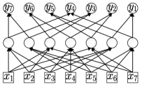
In particular, we focus on the message passing on a specific node. As shown in Fig. 1, the incoming messages to this node are expressed as a vector , where comes from the -th connecting edge, for each . Subsequently, the node computes outgoing messages, represented as , where is the outgoing message sent back to the -th connecting edge and denotes a general function for computing outgoing messages. Note that when computing , the function does not include as input. This is a well-known computation principle in message passing algorithms to avoid propagating ’s messages back to it again.

For any , the processing of computing can be abstracted as a directed rooted tree (DRT), whose root is and leaves are excluding . In such a DRT, each -input internal node corresponds to an -input operator. For example, assume and . The computation of can be handled by the seven DRTs shown in Fig. 2. The processing of computing can be represented as , corresponding to the first DRT in Fig. 2. The computation of any other is analogous, and all these DRTs can be handled in parallel. As a result, the complexity for computing by such seven DRTs can be measured by fourteen 3-input and seven 2-input nodes, and the latency can be measured by one 3-input and one 2-input nodes.
In fact, we can reuse the computation units corresponding to the same subtree among different DRTs, so that the complexity can be reduced under the same latency. Formally, we use a class of graphs, called structure to represent this process. For instance, the seven DRTs in Fig. 2 can be united into the structure in Fig. 3, such that this structure realizes the same computation of but requires lower complexity under the same latency. More specifically, the complexity of the structure can be measured by eight 3-input and seven 2-input nodes. We remark that, the structure in Fig. 3 was indeed proposed in [17] for efficiently implementing the node update in stochastic LDPC decoders.


However, the latency and complexity may vary in different structures. For example, the computing process corresponding to the structure in Fig. 4 can also obtain with . The complexity of the structure can be measured by seven 3-input and seven 2-input nodes, and the latency can be measured by one 3-input and one 2-input nodes. Therefore, under the same latency, the structure has a lower complexity (one less 3-input node) than that in Fig. 3. It is always of significant interest to find structures with lower complexity/latency. To this end, we [18] investigate a class of binary-input structures, but the systematic construction of low complexity and/or low latency muti-input structures remains open. Here “multi-input” means that there may exist -input computation nodes for any , where is the maximum number of inputs for a node and it should be regarded as a preset and fixed integer throughout this paper.
In this paper, we focus on low complexity/latency multi-input structures for computing from . Specifically, we propose two classes of multi-input structures for different scenarios:
-
•
For the scenario where complexity has a higher priority than latency, we propose a class of structures, called star-tree-based structures. Among these structures, we derive algorithms for computing their lowest complexity as well as the lowest latency of the complexity-optimal structures. We derive an algorithm to obtain the complexity-optimal ones of such structures, and illustrate that they have the near-lowest (and sometimes the lowest) complexity among all structures. We further derive an algorithm to obtain the latency-optimal ones among the complexity-optimal star-tree-based structures.
-
•
For the scenario where latency has a higher priority than complexity, we propose a class of structures, called isomorphic-DRT-based structures. We derive an algorithm to obtain the latency-optimal ones of such structures, and prove that they have the lowest latency among all structures. We further develop a construction for the complexity-optimal ones among the latency-optimal isomorphic-DRT-based structures.
The remainder of this paper is organized as follows. Firstly, Section II presents preliminaries related to graphs and trees. Next, Section III defines the structures under consideration for node computation in this paper. Then, Sections IV and V delve into star-tree-based and isomorphic-DRT-based structures, respectively. Finally, Section VI concludes this paper.
II Preliminaries
In this section, we introduce preliminaries regarding graphs and trees, mainly based on [19]. For convenience, define as the set of non-negative integers. For any with , define and . For any , let be a vector of length whose -th entry is 1 and other entries are 0.
II-A Graphs
A graph, denoted as , consists of a node set and an edge set . Any element in is called a directed (resp. undirected) edge which is denoted by an ordered (resp. unordered) pair . The term “ordered” (resp. “unordered”) implies that (resp. ). A graph is a directed (undirected) graph if and only if (iff) each element in is a directed (undirected) edge. When graphically represented, directed edges are depicted using arrows, whereas undirected edges are depicted using lines. A graph is called a subgraph of if .
In a directed graph , an edge is referred to as a leaving or outgoing edge of node , and an entering or incoming edge of node . In contrast, for an undirected graph , the edge is simply described as an edge of and . To describe the operations of removing or adding a node or an edge from/to a graph , we utilize the notation of subtraction/addition (represented by ). Specifically, , , , and .
For any graph and node , define as the degree of in . If is an undirected graph, is the number of edges connecting with . If is a directed graph, is the number of incoming edges of . For any graph and , define as the number of degree- nodes in . For any graph , define as the degree vector of , where for each , if is undirected and if is directed.
We call node sequence a path in iff , where is called the length of . Moreover, is called a simple path iff . For any , we say that is reachable from if there exists a path from to . The distance from to is defined as the length of the shortest path from to . If no such path exists, the distance is regarded as . We further call a cycle if , , , and is a simple path.
For any directed graph , we call a directed acyclic graph (DAG) iff there exists no cycle in . For any DAG and , define as a subgraph of . Moreover, we define . An undirected graph is connected if every node is reachable from all other nodes.
II-B Trees
A tree is defined as a connected, acyclic, undirected graph. Given any tree and any node , we call a leaf of if its degree . Otherwise, we call an internal node.
A rooted tree is a tree in which there is a unique node called the root of the tree. We consider a rooted tree , with its root denoted by . The depth of any node is defined as the distance between and . Additionally, for a non-negative integer , denote the -th level as the set of all the nodes with the depth . The height of is determined by the greatest depth among all its nodes. For any edge , if the depth of is greater than the depth of , then is designated as the parent of , and conversely, is the child of .
The directed variant of a rooted tree , say , is created by converting each undirected edge , where is a child of , into a directed edge from to in . We refer to as a directed rooted tree (DRT), with being its undirected counterpart. For any node , is called the subtree of rooted at . For any , let , where is the result (a DRT) by making as a DRT with root . Let .
II-C Labels of Graphs
For any graph , we call a labelled graph iff every node in is given a unique label (as a result, each edge is also given a unique label). Conversely, if not all nodes in are uniquely labelled, is termed a partially unlabelled graph.
Two labelled graphs and are considered identical, i.e., , iff and have same labelled nodes and edges (and root for rooted trees). Meanwhile, two partially unlabelled graphs, and , are deemed identical if there exists a labelling scheme for the unlabelled nodes in both and that renders them labelled and identical.
Two partially unlabelled graphs and are the same iff there exists a way to label all unlabelled nodes in and such that and become labelled and the identical. Graphs and are isomorphic if there is a way to reassign labels to all nodes in both graphs, resulting in identically labelled and .
III Structures for Node Computation
Recall that and represent the incoming and outgoing messages, respectively. In this paper, we focus on the scenario where for each , a DRT is employed to delineate the computation of from excluding . Specifically, within , the leaves correspond to the incoming messages excluding , the internal nodes correspond to operations whose number of inputs is between 2 and , and the root corresponds to . Some examples of such DRTs for are depicted in Fig. 2.
Define an input set and an output set , where node (resp. ) corresponds to the -th incoming message (resp. outgoing message ). In this paper, we remark that for any graph and any node , is labelled in iff is an input node from or an output node from . Consequently, is partially unlabelled if . To describe the computation process, we introduce the structure defined as follows.
Definition 1.
For any DAG , we say that is a structure with input size iff fulfills the following properties.
-
1)
contains nodes with no incoming edges, which are exactly .
-
2)
contains nodes with no outgoing edges, which are exactly .
-
3)
For , is a DRT whose leaves are exactly .
-
4)
For two different nodes , .
-
5)
For any node , we have .
We remark that Definition 1 corresponds to [18, Definition 2] in a special case where . For any , define as the set of all structures with input size . We may sometimes use subsets of a structure, referring to as substructures, which is defined below.
Definition 2.
A DAG is called a substructure iff there exists a structure satisfying that . For any two substructures and , denote the union of and by , where only one copy of the same subtrees is kept, corresponding to the fourth property of Definition 1.
According to Definition 2, for any two substructures and , is still a substructure if . Moreover, for any structure , is a substructure of , and always holds. A more specific example is that, the seven DRTs depicted in Fig. 2 are substructures whose union (under the operation ) results in the structure in Fig. 3.
In practice, each degree- node corresponds to an -input computation unit, the complexity and latency of which should increase as increases. Therefore, we define the complexity factor and latency factor to describe this fact. Specifically, for each , denote and respectively as the complexity factor and latency factor of the -input computation node. The complexity and latency factors are determined by the actual situation of the hardware. In particular, and are set to 0, and it is reasonable to assume and for . Accordingly, we can define the complexity and latency of a substructure (as well as structure) as follows.
Definition 3.
For any substructure , the complexity of , denoted by , is defined as the weighted number of nodes in :
Definition 4.
For any substructure , the latency of is defined as
where is a path in and is the latency of .
As an example, the complexity and latency of the structure in Fig. 4 are and , respectively. It is reasonable to use complexity and latency as two key criteria for evaluating the performance of a structure. In this paper, our main purpose is to discover the structures with low complexity and/or latency.
IV Star-Tree-Based Structures
In this section, we construct structures for the scenario where complexity has a higher priority than latency. To this end, we focus on a class of structures, called star-tree-based structures, which probably have the (near) lowest complexity among all structures. Specifically, Section IV-A proposes a class of trees, called star trees, and further presents a one-to-one mapping between star trees and star-tree-based structures. Next, Section IV-B establishes a necessary and sufficient condition between degree vectors and the existence of star trees. Thus, the complexity of a star-tree-based structure is completely determined by the degree vector of the corresponding star tree. Therefore, Theorem 1 is proposed to find the degree vectors that lead to the complexity-optimal star-tree-based structures. Finally, Section IV-C derives Theorem 2 to find a latency-optimal star-tree-based structure corresponding to a given degree vector . As a result, if is the uniquely optimal degree vector obtained from Theorem 1, then is a complexity-optimal star-tree-based structure which also has the lowest latency among all complexity-optimal star-tree-based structures.
IV-A Star Trees and Star-Tree-Based Structures
In this subsection, we propose a class of trees, called star trees, in Definition 5. Next, Construction 1 and Lemma 1 illustrate that, based on any star tree , we can obtain a low complexity structure, denoted as , which is called a star-tree-based structure.
Definition 5 (star trees).
An -input star tree is an (undirected) tree fulfilling the following properties.
-
•
has leaves, which are exactly .
-
•
The degree of each internal node in is between 3 and .


Denote as the set of all -input star trees. For example, Fig. 5 shows the only star tree in , and Fig. 6(a) shows a star tree in . In fact, we can obtain a structure based on any star tree. For instance, consider the star tree in Fig. 6(a). First, making as the root and changing undirected edges to directed ones can lead to the DRT in Fig. 6(b). Second, removing and labelling the new root as can result in the DRT in Fig. 6(c) which could be used for computing from . Third, proceed the above steps by replacing and with and , respectively, leading to the seven DRTs in Fig. 7. Finally, these DRTs can be united (under the union operation ) to the structure in Fig. 8. We formally describe the construction from star trees to structures in Construction 1, and use Lemma 1 to state the correctness of the construction.

Construction 1.
Given a star tree , return
as the constructed star-tree-based structure corresponding to , where is a DRT defined in Section II-B.
All the structures derived from star trees via Construction 1 are called star-tree-based structures. For example, considering and the star tree in Fig. 6(a), the DRTs correspond to the seven DRTs in Fig. 7, and the star-tree-based structure corresponds to the structure in Fig. 8.
Lemma 1.
For any and , then .
Proof:
For any , and , is a leaf in . Let be the only edge of . is a DRT with root and leaves . As a result, we have . ∎

According to Lemma 1, Construction 1 is a one-to-one mapping from star trees to star-tree-based structures. As shown in Fig. 8, each computation node is either reachable to or reachable from , for any . Noting that in any structure, a node reachable from can never be contained in the DRT rooted at , the computation nodes in Fig. 8 have been contained in as many DRTs in Fig. 7 as possible, indicating that they are fully reused. In particular, it was proved in [18] that for , the star-tree-based structures have the lowest complexity among all the binary-input structures. This implies that for , star-tree-based structures are likely to have the near-lowest (and sometimes the lowest) complexity among all structures. We thus focus on star-tree-based structures in this section.
IV-B The Lowest Complexity of Star-Tree-Based Structures
In this subsection, first, Lemma 2 illustrates that the complexity of a star-tree-based structure is totally determined by the degree vector of the corresponding star tree. Next, Lemma 3 establishes a necessary and sufficient condition between degree vectors and the existence of a star trees. Based on these preparations, we finally formulate Problem 1 and then solve it in Theorem 1, aiming to obtain complexity-optimal star-tree-based structures via optimizing degree vectors.
Lemma 2.
For any , the complexity of is
| (1) |
where denotes the number of degree- nodes in and is the complexity factor of -input nodes.
Proof:
Recall that the degree vector of is . Therefore, Lemma 2 indicates that is fully determined by . We are interested in optimizing degree vectors to generate complexity-optimal star-tree-based structures. Since Construction 1 establishes a one-to-one mapping between star trees and star-tree-based structures, the remaining question is that what degree vectors can result in valid -input star trees. The following lemma answers this question.
Lemma 3.
For any , there exists a star tree with degree vector iff
| (2) |
Proof:
Necessity: Let . We prove that the degree vector of satisfies (2). Firstly, for , there exists only one star tree as shown in Fig. 5, and (2) holds obviously. Secondly, for , assume (2) holds for any . We attempt to prove (2) holds for in the following. If contains only one internal node, (2) holds obviously. If contains at least two internal nodes, there always exists an internal node that connects with one internal node and leaves. Without loss of generality, denote the leaves connecting with as , respectively. Then, let , and relabel as . We can verify that . Since (2) holds for , we have , leading to , i.e., (2) holds for . Therefore, the necessity is proved.
Sufficiency: Suppose the degree vector satisfies (2). We provide Construction 2 to prove that there always exists a star tree with degree vector .
Construction 2.
For a given degree vector , we construct a star tree by the following steps.
Step 1: Select a . Then, we can construct an undirected tree , which contains one degree- internal node and leaves. Decrease by 1.
Step 2: If , go to Step 3. Otherwise, select a and select an arbitrary leaf . Connect new leaves to . We still use to denote the new tree and decrease by 1. Repeat Step 2.
Step 3: Label the leaves in as and keep the internal nodes unlabelled. Return as the constructed star tree.
∎
For any , there exists at least one degree vector satisfying (2) and to generate star tree via Construction 2. Note that it may result in multiple star trees, since there are multiple feasible choices of from in Steps 1 and 2. Combining with Lemma 1, corresponds to multiple star-tree-based structures. Denote as the set of all the star-tree-based structures derived from . Since the complexity of any structure in is the same by Lemma 2, it suffices to optimize degree vectors to generate complexity-optimal star-tree-based structures. Specifically, define as the minimum complexity of star-tree-based structures with input size . Computing is equivalent to solving the following optimization problem.
| Problem 1: | ||||
The left problem is to solve Problem 1, which can be done in Algorithm 1. The following theorem illustrates the correctness and time complexity of Algorithm 1.
Theorem 1.
can be computed by Algorithm 1 with time complexity .
Proof:
In Algorithm 1, as shown in Line 1, we have , since and for , and no computation nodes are required. Then, for any , assume is an optimal solution to Problem 1 for . For any with , let , where is a vector with length whose -th entry is 1 and other entries are 0. Then is an optimal solution for , leading to . Therefore, holds, corresponding to Line 3 of Algorithm 1.
By Algorithm 1, we are able to determine the lowest complexity of star-tree-based structures with input size . Further by backtracking, we can obtain an (or all if needed) optimal degree vector which leads to complexity-optimal star-tree-based structures . However, the structures in may have different latency. We are interested in further obtaining the latency-optimal structures in in the following subsection.
IV-C The Lowest Latency of Star-Tree-Based Structures for Given Degree Vectors
In this subsection, first, Lemma 4 defines the latency of star trees and shows that it can fully characterize the latency of the corresponding star-tree-based structures. Then, Lemma 5 illustrates how to compute the latency of star trees. Based on these preparations, we finally formulate Problem 2 and then solve it in Theorem 2, aiming to obtain the latency-optimal structures in via minimizing the latency of star trees corresponding to a given degree vector .
Lemma 4.
For any star tree , define
as the latency of . Then, .
Proof:
Assume the star tree . Obviously, there exists a simple path iff there exists a path , where for each . As a result, we have . ∎
As shown in Lemma 4, minimizing the latency of structures derived from the star trees with a given degree vector is equivalent to minimizing the latency of the star trees. The following lemma shows how to compute the latency of a star tree.
Lemma 5.
Proof:
Suppose is a simple path in such that . There always exists an such that (5) holds for and . This completes the proof of (5).
We are now to prove (6). Suppose is an arbitrary edge satisfying (5). According to Definition 4, (resp. ) denotes the latency of the path in (resp. ) from a leaf to (resp. ), and we let this leaf be (resp. ), without loss of generality. Then, we have , where is a simple path in with and . Therefore, we have .
To prove (6), it now suffices to prove . Let , be two arbitrary leaves in such that there exists a simple path connecting them and the path’s latency is . If and or and , we have . If , we have . If , we have . Therefore, . ∎
Lemma 5 indicates that, the minimum latency of star trees with degree vector is equal to the minimum value of , where and are two DRTs (respectively corresponding to and in Lemma 5) satisfy the following three conditions: (i) , (ii) , and (iii) , i.e., the summation of and ’s degree vectors equals . As a result, computing , the minimum latency of the star-tree-based structures derived from degree vector , is equivalent to solving the following optimizing problem.
| Problem 2: | |||||
| (7) | |||||
| (8) | |||||
| (9) |
To this end, for any degree vector and positive integer , define , where are DRTs and the summation of their degree vectors equals . Here, returns the lowest latency of the substructures that have the degree vector and consist of disjoint DRTs. It will be computed later in Algorithm 3. For any two degree vectors , , we say iff for each , . Then, we can solve Problem 2 by Algorithm 2.
Theorem 2.
Given a degree vector and , , Algorithm 2 can compute with time complexity .
Proof:
Let be the degree vector of and be the degree of ’s root. According to constraint (9), the degree vector of must be . Therefore, as shown in Lines 2–13, by traversing and from 1 to , we can enumerate all the feasible solutions and find the one with lowest . Specifically, given and , the minimum latency of and are and respectively, and the conditions in Line 7 correspond to the constraints (7) and (8).
At this point, the left problem is to compute , . We complete this task in Algorithm 3.
Lemma 6.
Given a degree vector , then can be computed by Algorithm 3 with time complexity .
Proof:
Firstly, as shown in Line 2, for any , we have , since there exist no computation nodes in the graph. Then, for any degree vector and , suppose is an arbitrary substructure that has degree vector and consists of disjoint DRTs. If , the substructure is a DRT. Fixing the degree of its root as , the graph has degree vector and consists of disjoint DRTs. Therefore, when fixing , the minimum latency of is . As shown in Line 7, by traversing all the possible , we can find the minimum latency of :
| (10) |
If , the substructure consists of disjoint DRTs, named . Fixing the degree vector of as , the graph has degree vector and consists of disjoint DRTs. Therefore, when fixing the degree vector of as , the minimum latency of is . As shown in Line 7, by traversing all the possible , we can find the minimum latency of :
| (11) |
As shown in Lines 4–10, we enumerate all the possible and and compute . Here, we enumerate such that is non-decreasing and enumerate from 1 to , so that when computing , the required values of have been already computed. Therefore, given , Algorithm 3 can obtain .
In the following, we investigate the time complexity of Algorithm 3. In Line 4, we enumerate . In Line 5, we enumerate from to . And in Line 9, we enumerate . Thus, the number of computations is . We can simplify it as follows:
The proof is completed. ∎
By Algorithms 2 and 3, we are able to determine the lowest latency of the star-tree-based structures derived from degree vector . Further by backtracking, we can find the corresponding latency-optimal star tree with degree vector , and can be further used to generate a latency-optimal star-tree-based structure from via Construction 1. Note that can be any valid degree vector. However, if is the uniquely optimal solution to Problem 1, has the lowest latency among all the complexity-optimal star-tree-based structures. On the other hand, if Problem 1 has multiple optimal solutions, we can enumerate them to find the latency-optimal ones among complexity-optimal star-tree-based structures.
V Isomorphic-DRT-Based Structures
In this section, we construct structures for the scenario where latency has a higher priority than complexity. To this end, we focus on a class of structures, called isomorphic-DRT-based structures. Since there always exist isomorphic-DRT-based structures (or structures derived from them) achieving the lowest latency, which is explicated in Lemma 8. Section V-A proposes a class of DRTs, called isomorphic DRTs, and further provides a construction from isomorphic DRTs to isomorphic-DRT-based structures. Next, Section V-B presents a construction from type vectors to isomorphic-DRTs. Here, the type vector is used to characterize an isomorphic DRT, each component of which is the number of levels that contain nodes with the corresponding degree. We further illustrate that given a type vector, the latency of its corresponding isomorphic-DRT-based structures is uniquely determined. Therefore, Theorem 3 is proposed to find the type vectors that lead to the latency-optimal isomorphic-DRT-based structures. Finally, Section V-C derives Construction 5 and Theorem 4 to find a complexity-optimal isomorphic-DRT-based structure corresponding to a given type vector . As a result, if is the uniquely optimal type vector obtained from Theorem 3, then is a latency-optimal isomorphic-DRT-based structure which also has the lowest complexity among all latency-optimal isomorphic-DRT-based structures.
V-A Isomorphic DRTs and Isomorphic-DRT-Based Structures
In this subsection, we propose a class of DRTs, called isomorphic DRTs, in Definition 6. Then, Construction 3 and Lemma 7 show that, based on any isomorphic DRT , we can obtain a structure, which is called an isomorphic-DRT-based structure. Finally, Lemma 8 illustrates that it suffices to investigate the isomorphic-DRT-based structures when the latency of structures is of interest.
Definition 6 (isomorphic DRT).
We refer to a DRT as an isomorphic DRT iff for any internal node in , all the subtrees rooted at ’s children are isomorphic.
Denote as the set of all isomorphic DRTs with exactly -leaves. Fig. 2 shows an example of isomorphic DRTs in . In an isomorphic DRT , the nodes in a same level have the same degree (number of incoming edges). For the sake of convenience, for any , we refer to a level of by type- level if it contains degree- nodes. Moreover, we define the type vector of by , where is the number of type- levels in .
In the following, we propose a construction from isomorphic DRTs to structures in Construction 3, and use Lemma 7 to state the correctness of the construction.
Construction 3.
For any and an isomorphic DRT , we construct the structure by the following steps:
Step 1: For any , let be a copy of , and label all the leaves of as respectively.
Step 2: Return as the constructed structure.
Lemma 7.
For any and , supposing that is a structure derived from via Construction 3, then .
All the structures that can be derived from isomorphic DRTs via Construction 3 are called isomorphic-DRT-based structures. Fig. 3 shows an example of isomorphic-DRT-based structure corresponding to the isomorphic DRTs given in Fig. 2. Note that the resultant structure of Construction 3 is generally not unique for a given isomorphic DRT , since we may label the leaves of in different ways. For convenience, denote as the set of all possible isomorphic-DRT-based structures derived from via Construction 3.
In the following, we illustrate that the minimum latency of the structures for given can be connected to the minimum latency of isomorphic-DRT-based structures with input size .
Lemma 8.
For any , there always exists an isomorphic-DRT-based structure satisfying that and .
Proof:
For a given structure , we attempt to construct an isomorphic-DRT-based structure satisfying that and by the following steps.
Step 1: Let denote the DRT and then unlabel . Set .
Step 2: Let be the set of nodes in the -th level of . If all the nodes in are leaves, go to Step 3. Otherwise, select a node , such that the number of leaves of is equal to or greater than . Then, for each , modify the , so that is isomorphic to . Increase by 1 and then repeat Step 2.
Step 3: Return derived from via Construction 3.
In Step 2, the number of ’s leaves is either increased or unchanged, and the latency of is at most . As a result, is an isomorphic-DRT-based structure satisfying that and . The proof is completed. ∎
According to Lemma 8, it suffices to investigate the latency-optimal isomorphic-DRT-based structures whose number of leaves is at least when the minimum latency of is of interest. In particular, if we can first construct a latency-optimal isomorphic-DRT-based structure with , then properly we remove certain nodes (including , ) from to obtain a latency-optimal structure , where by Lemma 8 and by the fact that removing nodes from does not increase latency. For instance, we can initially construct the latency-optimal isomorphic-DRT-based structure shown in Fig. 4, and then remove the nodes and from to obtain the latency-optimal shown in Fig. 9.
According to the above analysis, we only focus on the latency and complexity of isomorphic-DRT-based structures in the rest of this section,.

V-B The Lowest Latency of Isomorphic-DRT-Based Structures
In this subsection, first, Lemma 9 investigates the latency of isomorphic-DRT-based structures and find that given a type vector, the latency of its corresponding isomorphic-DRT-based structures is uniquely determined. Next, Construction 4 provides a method to obtain isomorphic DRTs for given type vectors. Based on these preparations, we finally formulate Problem 3 and solve it in Theorem 3, aiming to obtain latency-optimal isomorphic-DRT-based structures via optimizing type vectors.
Lemma 9.
For any , and , the latency of is
| (12) |
where denotes the number of type- levels in and is the latency factor of -input nodes.
Proof:
According to Lemma 9, the latency is fully determined by the type vector . We are interested in optimizing type vectors to generate latency-optimal isomorphic-DRT-based structures. Since Construction 3 can generate isomorphic-DRT-based structures from isomorphic DRTs, the remaining question is that what type vectors can result in valid -input isomorphic DRTs. The following lemma answers this question.
Lemma 10.
For any , there exists an isomorphic DRT with type vector iff
| (13) |
Proof:
Necessity: According to Definition 6, the necessity holds obviously.
Sufficiency: Suppose the type vector satisfies (13). We provide Construction 4 to prove that there always exists an isomorphic DRT with type vector .
Construction 4.
For a given type vector , we construct an isomorphic DRT by the following steps.
Step 1: Select a . Then, we can construct a DRT , which contains one degree- internal node and leaves. Decrease by 1.
Step 2: If , return as the constructed isomorphic DRT. Otherwise, select a and replace each leave in with a subtree that contains one degree- internal node and leaves. Repeat Step 2.
∎
Note that for some , there may exist no type vector satisfying (13) such that . However, as discussed at the end of Section V-A, we only need to focus on those such that (13) can be satisfied and . Further recall that a type vector can generate multiple isomorphic DRTs via Construction 4 and an isomorphic DRT can also generate multiple isomorphic-DRT-based structures via Construction 3. As a result, a type vector corresponds to multiple isomorphic-DRT-based structures. Denote as the set of all the isomorphic-DRT-based structures derived from degree vector . Since the latency of any structure in is the same by Lemma 9, it suffices to optimize type vectors to generate latency-optimal isomorphic-DRT-based structures. Specifically, define for , which is the minimum latency of isomorphic DRTs with input size as well as the minimum latency of isomorphic-DRT-based structures with input size . Computing is equivalent to solving the following optimization problem.
| Problem 3: | |||||
| (14) |
The left problem is to solve Problem 3, which has been done in Algorithm 4. The following theorem illustrates the correctness and time complexity of Algorithm 4.
Theorem 3.
can be computed by Algorithm 4 with time complexity .
Proof:
In Algorithm 4, as shown in Line 1, we have , since no computation nodes are required. Then, for any , assume is an optimal solution to Problem 3 for . For any integer satisfying , then must be a factor of . Let , where is a vector with length whose -th entry is 1 and other entries are 0. Then we have is an optimal solution for , leading to . Therefore, holds, corresponding to Line 3 of Algorithm 4.
By Algorithm 4, we are able to determine the lowest latency of isomorphic-DRT-based structures with input size . Further by backtracking, we can obtain an (or all if needed) optimal type vector which leads to latency-optimal isomorphic-DRT-based structures . However, the structures in may have different complexity. We are interested in further obtaining the complexity-optimal structures in in the following subsection.
V-C The Lowest Complexity of Isomorphic-DRT-Based Structures for Given Type Vectors
In this subsection, for a given degree vector , we first generate an isomorphic-DRT-based structure via Construction 5, and then prove that has the lowest complexity among all isomorphic-DRT-based structures in Theorem 4.
Construction 5.
For a given type vector , we construct a structure by the following steps.
Step 1: Obtain an isomorphic DRT from via Construction 4.
Step 2: Obtain an isomorphic-DRT-based structure from via Construction 3, where for each , label leaves of from left to right in a consecutive way: , where and are considered as consecutive to each other. Return as the constructed structure.
Fig. 4 shows a structure obtained from Construction 5 for , and . The following theorem states that does have the lowest complexity among .
Theorem 4.
For a given type vector and , let be the structure obtained from Construction 5. Then, and .
Proof:
Let . We first prove
| (15) |
For any , must be an isomorphic DRT of height , where . For , let be the -th level in , i.e., any node iff the distance from to some output node in is . As a result, . Since is an isomorphic-DRT-based structure, the nodes in have the same degree, which is referred to as . Our idea is to prove such that .
For any , let , where for any , if and otherwise. Meanwhile, for any and , let , where is the component-wise XOR operation. If , let ( zeros in total). Moreover, let .
On the one hand, for any and with even , we have , where is the -th child of in for . That is, . On the other hand, for any with even , we have , where for any , if and otherwise. This leads to . As a result, we have , implying that as well as (15).
Let be the returned structure in Construction 5. Obviously, . Given (15), it suffices to prove to complete the proof of Theorem 4. Let denote the -th level of . By Construction 5, all DRTs , are isomorphic to each other and the leaves of each are labelled in a consecutive way, implying that . Then, follows. ∎
We remark that for , any isomorphic DRT is a perfect DRT that was considered in [18]. As a result, Theorem 4 can be thought as an extension of [18, Theorem 6] from to . Note that can be any valid degree vector. However, if is the uniquely optimal solution to Problem 3, has the lowest complexity among all the latency-optimal isomorphic-DRT-based structures. On the other hand, if Problem 3 has multiple optimal solutions, we can enumerate them to find the complexity-optimal ones among latency-optimal isomorphic-DRT-based structures.
VI Conclusion
In this paper, we have investigated the structures that can be used by a node in a message passing algorithm to compute outgoing messages from incoming messages. Specifically, for the scenario where complexity has a higher priority than latency, we proposed a class of structures, called star-tree-based structures. Within this framework, we derived algorithms to determine both the lowest achievable complexity and the corresponding lowest latency for these optimized structures. Next, for the scenario where latency has a higher priority than complexity, we proposed a class of structures termed isomorphic-DRT-based structures. We derived an algorithm to ascertain the lowest latency achievable with these structures and constructed latency-optimal isomorphic-DRT-based structures with the lowest complexity. Notably, our findings extend the work presented in [18] to accommodate multi-input scenarios. Our future work is to investigate optimal/near-optimal structures that can achieve a good tradeoff between complexity and latency.
References
- [1] T. J. Richardson and R. L. Urbanke, Modern Coding Theory. Cambridge University Press, 2008.
- [2] F. R. Kschischang, B. J. Frey, and H. Loeliger, “Factor graphs and the sum-product algorithm,” IEEE Trans. Inf. Theory, vol. 47, no. 2, pp. 498–519, 2001.
- [3] I. Arasaratnam and S. Haykin, “Cubature kalman filters,” IEEE Trans. Autom. Control., vol. 54, no. 6, pp. 1254–1269, 2009.
- [4] W. Xu and F. Zhang, “FAST-LIO: A fast, robust lidar-inertial odometry package by tightly-coupled iterated kalman filter,” IEEE Robotics Autom. Lett., vol. 6, no. 2, pp. 3317–3324, 2021.
- [5] X. Yu and Z. Meng, “Robust kalman filters with unknown covariance of multiplicative noise,” IEEE Trans. Autom. Control., vol. 69, no. 2, pp. 1171–1178, 2024.
- [6] J. Gauvain and C. Lee, “Maximum a posteriori estimation for multivariate gaussian mixture observations of markov chains,” IEEE Trans. Speech Audio Process., vol. 2, no. 2, pp. 291–298, 1994.
- [7] N. M. Ghahjaverestan, S. Masoudi, M. B. Shamsollahi, A. Beuchee, P. Pladys, D. Ge, and A. I. Hernández, “Coupled hidden markov model-based method for apnea bradycardia detection,” IEEE J. Biomed. Health Informatics, vol. 20, no. 2, pp. 527–538, 2016.
- [8] C. Guo, Z. Liang, J. Zeng, M. Song, and Z. Xue, “A predictive hidden semi-markov model for bridges subject to chloride-induced deterioration,” in 21st IEEE International Conference on Software Quality, Reliability and Security, QRS 2021 - Companion, Hainan, China, December 6-10, 2021. IEEE, 2021, pp. 751–756.
- [9] S. Sun, C. Zhang, and G. Yu, “A bayesian network approach to traffic flow forecasting,” IEEE Trans. Intell. Transp. Syst., vol. 7, no. 1, pp. 124–132, 2006.
- [10] J. Zeng, G. Zhou, Y. Qiu, C. Li, and Q. Zhao, “Bayesian tensor network structure search and its application to tensor completion,” Neural Networks, vol. 175, p. 106290, 2024.
- [11] R. G. Gallager, “Low-density parity-check codes,” IRE Trans. Inf. Theory, vol. IT-8, no. 1, pp. 21–28, Jan. 1962.
- [12] D. MacKay, “Good error-correcting codes based on very sparse matrices,” IEEE Trans. Inf. Theory, vol. 45, no. 2, pp. 399–431, 1999.
- [13] T. J. Richardson and R. L. Urbanke, “The capacity of low-density parity-check codes under message-passing decoding,” IEEE Trans. Inf. Theory, vol. 47, no. 2, pp. 599–618, Feb. 2001.
- [14] 3GPP, “NR; Multiplexing and channel coding,” Release 15, Technical Specification (TS) 38.212, 2017.
- [15] Y. Ding, X. He, K. Cai, G. Song, B. Dai, and X. Tang, “An efficient joint decoding scheme for outer codes in DNA-based data storage,” in Proc. IEEE/CIC Int. Conf. Commun. China Workshops, Aug. 2023, pp. 1–6.
- [16] J. Chen, A. Dholakia, E. Eleftheriou, M. P. Fossorier, and X.-Y. Hu, “Reduced-complexity decoding of LDPC codes,” IEEE Trans. Commun., vol. 53, no. 8, pp. 1288–1299, Aug. 2005.
- [17] Y.-L. Ueng, C.-Y. Wang, and M.-R. Li, “An efficient combined bit-flipping and stochastic LDPC decoder using improved probability tracers,” IEEE Transactions on Signal Processing, vol. 65, no. 20, pp. 5368–5380, 2017.
- [18] X. He, K. Cai, and L. Zhou, “A class of optimal structures for node computations in message passing algorithms,” IEEE Trans. Inf. Theory, vol. 68, no. 1, pp. 93–104, Jan. 2022.
- [19] T. H. Cormen, C. E. Leiserson, R. L. Rivest, and C. Stein, Introduction to Algorithms: 3rd Edition. Cambridge, MA, USA: MIT Press, 2009.