Tuning the critical Li intercalation concentrations for MoX2 bilayer phase transitions
Abstract
Transition metal dichalcogenides (TMDs), such as MoS2, are known to undergo a structural phase transformation as well as a change in the electronic conductivity upon Li intercalation. These properties make them candidates for charge-tunable ion-insertion materials that could be used in electro-chemical devices. In this work we study the phase stability and electronic structure of H and T’ Li-intercalated MoX2 bilayers with X=S, Se, or Te. Using first-principles calculations in combination with classical and machine learning modeling approaches, we find that the H phase is more stable at low Li concentration for all X, and the critical Li concentration at which the T’H transition occurs decreases with increasing mass of X. Furthermore the relative free energy of the two phases becomes less sensitive to Li insertion with increasing atomic mass of the chalcogen atom X. While the electronic conductivity increases with increasing ion concentration at low concentrations, we do not observe a (positive) conductivity jump at the phase transition from H to T’.
I Introduction
Autonomous vehicles (AVs) will serve global energy security goals as they offer efficiency opportunities that could enable significant reduction in fuel consumption. Unfortunately, with the current technology the electrical power associated with on-board sensing and calculations for driving decisions could reach quite large values of the order of kW [1]. This is a consequence of the fact that silicon technology uses about a pJ/operation [2].
Neuromorphic computing is a novel computing architecture that holds the promise for advanced computing with high energy efficiency, while being well suited for artificial intelligence (AI) tasks. Neuromorphic computing could have a profound impact on computation for autonomous vehicles and other sectors that require edge computing. One route for realizing novel devices for neuromorphic computing is to leverage ionic/electronic transport properties in electro-chemical devices. However, a major roadblock in the development of electro-chemical devices is the lack of understanding of the fundamental mechanisms that lead to conductivity changes in the ion-insertion materials used in neuromorphic devices.
Recently, a novel electro-chemical device called a Li-Ion Synaptic Transistor for Low Power Analog Computing (LISTA) has been pioneered by Talin et al. [2]. LISTA is 3-terminal redox transistor which allows ion-insertion into a channel by applying a small gate voltage. Through reversible Li intercalation, the channel electronic conductance (synaptic weight) can be gradually changed. Hundreds of conducting states can be modulated in a controllable fashion with switching times (s) comparable to those measured in biological synapses [3, 4] and much lower power ( fJ/operation [2]) than Si-based CMOS transistors.
In order to take the proof-of-concept LISTA device to a scalable technology, it is important to understand how it works at a fundamental level. Despite progress on the experimental front, the mechanisms that lead to conductivity changes are not fully understood. In particular it is not clear how the structural and electronic properties of the ion-insertion material evolve as a function of ion concentration. For example, do ions intercalate into the channel in an ideal fashion, i.e gradually and with uniform concentration, or rather do they form co-existing domains of insulating and metallic phases with sizes that depend on gate voltage? This and related questions regarding the equilibrium and nonequilibrium intercalation regimes can be addressed computationally via mesoscopic modeling approaches [5]. However, such models require knowledge of the phase stability diagram as well as the electronic properties of the ion-insertion materials as function of (uniform) ion concentration. Such knowledge can be obtained from first-principles studies.
From a materials point of view, quasi-two dimensional layered systems are attractive due to their layered structure. Indeed, they can be very useful in electrochemical devices because the weak van der Waals interaction between layers facilitates ion intercalation. As such, layered systems can find applicability in electrode materials for batteries with high energy storage, for example. Transition metal dichalcogenides (TMDs), i.e. MoS2, MoSe2 or MoTe2, represent a particular class of layered materials. These materials undergo a structural phase transformation upon ion intercalation. This transition is accompanied by a change in the electronic conductivity, which makes TMDs candidates for charge tunable ion-insertion materials in electro-chemical devices for neuromorphic computing. Moreover, two-dimensional, few-layer TMDs are of interest for small-scale device fabrication which is desirable since the write energy per operation (resistance) increases with channel size [2]. While there is a large body work on ion intercalation in bulk TMDs [6, 7, 8] and ion adsorption on monolayer TMDs [9], fewer studies so far have focused on few-layer TMDs [10] such as bilayers [11, 12]. Of the few studies of bilayers, Pandey et al. [11] examined the phase transition of MoS2 induced by lithiation to a heterostructure involving a metallic phase. The later work of Lu et al. [12] also used ab initio simulations to examine the relative rotation of the bilayers as a means of controlling the band structure of Li intercalated MoS2.
In this work we perform a first-principles based study of the phase stability and electronic structure evolution of Li ion-intercalated MoS2, MoSe2, MoS2 bilayer TMDs. Changes in phase and the attendant changes in electronic structure in MoX2 bilayers have ramifications on the performance of neuromorphic and related devices utilizing these materials. We hypothesize that ab initio Density Functional Theory (DFT) can be integrated with machine learning to efficiently predict the phase stability and electronic structure evolution of ion-insertion layered materials. We explore this path, together with the more established cluster expansion method, to obtain thermodynamic properties, the phase stability diagram, and related electronic properties.
II Theoretical framework
TMDs may take several polytype forms, such as the semiconducting H phase, metallic T phase, and semimetallic T’ phase. In few-layer TMDs, the metallic T phase is unstable due to a Peierls distortion that dimerizes the metal atoms leading to the formation of the T’ phase [13]. Thus, we consider only two competing phases, namely H and T’ which are illustrated in Fig. 1. A large fraction of our computational effort consists on estimating the free energy of these competing phases, from which a phase diagram as a function of Li concentration will be constructed. Ultimately, this allows us to make predictions regarding the electronic conductivity of Li ion-intercalated bilayer TMDs as function of ion concentration.

II.1 Free energy and phase stability
To motivate our methodology a brief review of fundamental statistical mechanics is needed. The canonical, Helmholtz free energy is
| (1) |
where is Boltzmann’s constant, is temperature, and
| (2) |
is the partition function. In Eq. (2) the sum is over all possible configurations with lithium atoms, and the energy is energy of configuration relative to a chosen reference state. The ensemble average of a quantity can be computed via
| (3) |
For brevity we have suppressed the dependence of the free energy on the system stress as we focus on fully relaxed systems, i.e. at zero stress; and, as a consequence, we will refer to this ensemble as the NT ensemble. A minimum in indicates the most likely concentration of Li at a given . The difference between phases
| (4) |
indicates which phase is more stable and eliminates the dependence on a reference state.
The grand canonical free energy takes a similar form to in Eq. (1)
| (5) |
where the partition function is
| (6) |
In this case the sum is over all possible configurations from no Li, , up to at the saturation of all low energy sites. Again we employ relaxed systems and refer to this as the T ensemble. In the present context of intercalation we introduce the site occupancy fraction and the formation energy [14]
| (7) |
The grand canonical potential provides information regarding how many Li reside on/in the bilayer when in equilibrium with an environmental reservoir of lithium (as in an electrochemical device) at chemical potential . With the free energy the average Li site occupancy can be computed:
| (8) |
In these free energy expressions the contribution to the entropy comes entirely from the configurational degrees of freedom. We omit dependence on vibrational modes, electronic modes, etc. While the vibrational entropy can be significant, its contribution to the free energy difference between phases is expected to be minor; the variation of the vibrational entropy across phases of the same chemical species is typically small so that it does not affect significantly the relative phase stability [15, 14]. Similarly, while the configurational entropy may converge slowly with system size, its variation between chemically similar phases is expected to converge fast enough to make it tractable to compute with feasible DFT system/supercell sizes. We explore the validity of this assumption together with further details on approximating the ensemble average in Appendix A.
II.2 Method for obtaining total energies
To calculate the relative free energies and thus the phase diagram we need a set of energies that sample the configurational space of each phase. We obtain these from ab initio density functional theory (DFT) calculations and hence are limited to small systems with a fixed number of bilayer lattice atoms and varying number of intercalated lithium atoms. The configurational space of these small systems can be sampled exhaustively using a surrogate model of the energies and other quantities of interest as a function of the bilayer configuration. We explored a number of surrogate models including classical cluster expansion and a variety of machine learning methods.
II.2.1 Ab initio calculations
We calculate total energies as well as the electronic density of states (DOS) of Li ion-intercalated bilayer TMD structures within the framework of ab initio DFT using the VASP code [16]. We use projector augmented wave (PAW) pseudo-potentials [17] and treat the exchange and correlation terms within the generalized gradient approximation with the PBE parameterization [18]. The energy cutoff was set to 400 eV.
We consider bilayer structures where the two monolayers are rotated by 180∘ with respect to each other. The translational alignment between the two MoX2 monolayers is such that the Mo atoms are vertically aligned (refer to Fig. 1), since within our DFT parameter settings we find the energy for this configuration to be lower than for other alignments in the presence of Li-ion intercalation. In particular, this translational alignment yields for MoS2 a total energy (per a rectangular supercell that contains intercalated Li ion) meV lower than the corresponding lowest energy of the intercalated AA’ stacking (where the top layer’s Mo atoms are aligned with the bottom layer’s S atoms and viceversa [19, 12]).
We construct systems using supercells obtained by laterally replicating the rectangular unit cell of bilayer MoX2 with X=S, Se or Te. We use lateral replicas with lateral area of 1.41.2 nm2 and vacuum separation along the out-of-plane direction of more than Å. There are 32 Mo atoms and 64 X atoms in our supercells in the absence of ion intercalation, and lithium atoms at saturation () of the low energy sites.
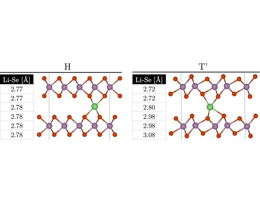
Even with only tens of sites, there is a large configurational space associated with Li ion intercalation in between the MoX2 monolayers of the bilayer. To explore the configurational space in order to compute ensemble averages, it is sufficient to sample only stable configurations as they carry most of the weight in Eq. (3) given that they correspond to local energy minima. For each phase we identify low energy ion-intercalation sites and select the most stable one, as we find that this crystallographic location has an energy several hundred meV lower than the other, metastable configurations. In the case of the H phase we find that the Li ion is most stable when positioned half-way in between two vertically aligned Mo atoms from different monolayers (see Fig. 2a)) [12]. This results in octahedral coordination to the X atoms (with bond length of about Å). In the T’ case the most stable Li site is not vertically aligned with Mo while coordination with the closest six X neighbors is distorted from the ideal octahedral case with four different bond lengths ranging from Å to Å (see Fig. 2b). We also checked in the MoS2 case for both phases that Li ion adsorption yields an energy significantly larger (by more than meV) than Li ion intercalation, hence the focus of this work is on ion intercalation.
The Li ion-intercalation sites in the 42 supercell form a 16-site layer sublattice, i.e. there is one possible Li intercalation site for each Mo2X4 bilayer formula unit. The Li-concentration in the stoichiometric formula LixMoX2 ranges from (no intercalation, , ) to at full (, ) Li sublattice occupancy. The number of possible configurations for fixed is . Summing over from to leads to 65,536 total configurations per system/phase. We do not consider mixtures of phases (domains) in a monolayer nor the possibility that two monolayers could belong to a different phase.
For each of the three MoX2 systems and for both H and T’ phases we randomly sample the configurational space such that the configurations with intercalated Li spanning the range from to are roughly equally represented. Each configuration is optimized by minimizing the stress tensor and relaxing the atomic forces to less than eV/ Å. During optimization the Brillouin zone is sampled with a 441 k-point grid. Convergence in the electronic density of states of the relaxed structures is achieved with a 10101 k-point grid. We do not include spin-orbit coupling due to the associated computational cost and because it is not expected to affect significantly the structural relaxation; we checked that spin-orbit coupling has an insignificant impact on the density of states near the Fermi level.
II.2.2 Surrogate models
Obtaining the total energy of all possible distinct initial configurations is computationally too expensive with ab initio DFT even for the relatively small 42 supercell. To this end we explore several surrogate models that can sample exhaustively the entire configurational space given DFT training data.
The first method we consider is cluster expansion (CE) [20, 21, 22], a classical technique based on a linear coefficient model with a nearest neighbor expansion
| (9) |
where the features are formed from a polynomial expansion of binned nearest neighbors . Here is the total number of neighbors in the -th bin. The bins we consider are annular rings with width small enough such that they contain one type of neighbor. In a -th order expansion are complete with powers of up to . The coefficients are found via regression to training data. In the standard form of CE, the polynomial order is set to ; we explored higher order polynomials as well.
We also used several machine techniques such as a basic multilayer perceptron (MLP) neural network (NN) as well as the more complex crystal graph convolutional neural network (CGCNN) [23] and image-based transfer learning with a convolutional neural network [24]. The MLP model is a feed-forward model of densely connected layers. The output of each preceding layer (starting with the selected inputs) is transformed by a linear weight matrix and then a non-linear activation function. The coefficients of the linear transformation of each layer comprise the parameters of the model. We trained the parameters of the MLP using the neighbor counts as inputs and the corresponding energies as outputs. The CGCNN formalism is more complex and is based on a universal and interpretable representation of crystalline materials. An input crystallographic structure is encoded as a graph whose nodes, corresponding to atoms, are connected by edges, corresponding to bonds, with surrounding atoms. The CGCNN architecture then applies a nonlinear graph convolution function that updates the atoms’ feature vectors with information from the surrounding atoms and bonds. A pooling layer then produces an overall feature vector for the entire crystal that satisfies invariance with respect to atom indexing (permutational invariance) and number of atoms in the unit cell (size invariance). Similar to the MLP training, we optimized the parameters of the CGCNN to fit the DFT predicted energy. We also applied a transfer learning technique using a pre-trained convolutional neural network (CNN), googlenet [25], originally used for image recognition. We replaced the classification last layer of this 22-layer deep CNN with a new regression layer and re-trained the network on predicting energies based on input images of the non-self-consistent electrostatic potential projected on a plane that passed through the unrelaxed Li-ion layer. The non-self-consistent electrostatic potential was selected since it is inexpensive to compute and the projection was necessary since googlenet operates on two-dimensional images.
For all these approaches the training set consisted of hundreds to thousands of input-output pairs. The inputs correspond to unrelaxed Li-intercalated MoX2 structures. Prior to the training models of the energy as a function of configuration, we transformed total energies obtained from DFT into formation energies according to a linear transformation Eq. (7). As seen in Fig. 3, this transformation reduces the energy range of the outputs by more than an order of magnitude, from about eV (the total energy decreases with increasing Li-site occupancy fraction because the Li intercalation energy is positive [12]) to about eV, facilitating better convergence during the training process.


III Results: phase stability and electronic structure evolution
With the methods described in the previous section we are able to calculate the free energy difference between the H and T’ phases of MoS2, MoSe2 and MoTe2 and estimate the phase transition as a function of Li site occupancy. Furthermore, we provide the DOS at the Fermi level to indicate where changes in conductivity occur with increasing Li occupancy.
III.1 Free energies and phase diagrams
Depending on the experimental conditions, the phase stability of Li ion intercalated bilayer TMDs should be computed with the closed system, NT, ensemble or the open system, T, ensemble. To this end, the calculated energies were used to construct the NT and T potentials as well as the statistical average of the Li site occupancy as function of Li chemical potential. Analysis of the errors induced by using a 42 system are detailed in Appendix A. This analysis indicates the finite size errors are negligible. Appendix B describes a comparison between the surrogate models in representing formation energies and DOS. Given the task of representing formation energies as a function of Li site occupancy, we show that classical cluster expansion (CE) is sufficient and competitive with the modern machine learning surrogate models we implemented in both accuracy and computational expense. The lower complexity CE model does well since the main input is the on-site occupancy of a small lattice and results in mean absolute errors (MAEs) of 50 meV. Compared to the MLP model with same features the main difference is a global polynomial basis for the CE model versus the piecewise basis of a typical NN. More sophisticated representations such as CGCNN or an image-based NN would differentiate themselves if the configurational space were more complex, for instance if there was significant rearrangement of the bilayer with relaxation.
Fig. 4 shows the NT free energy and T free energies for three Li ion intercalated bilayer systems: MoS2, MoSe2, and MoTe2, at room temperature =300 K. It appears that the T’ phase is preferred at high ion concentrations/low chemical potentials, as its free energy becomes lower than that of the H phase. Interestingly, as the chalcogen atom X gets heavier, the concentration range of stable T’ phases becomes larger and the threshold ion concentration where the H-T’ transition takes place gets smaller.


This trend can be clearly seen in Fig. 5 which shows the phase diagram at =300 K for the three bilayer systems. Fig. 5a shows that the stabilization energy (the free energy difference between T’ and H phases at ) decreases from eV/formula unit for MoS2, to eV/formula unit for MoSe2 and finally decreases to only eV/formula unit in the case of MoTe2. A similar trend has been discovered in the case of Li ion adsorption onto monolayer MoX2 [13]. Besides the stabilization energy, the threshold Li concentration where the HT’ transition happens decreases as well, from ions/formula unit for MoS2, to ions/formula unit for MoSe2 and finally to ions/formula unit in the case of MoTe2. (Recall .) The total change in free energy from zero occupancy to site saturation decreases with the mass of X, from eV/formula unit for MoS2, to 0.5 eV/formula unit for MoSe2, to 0.25 eV/formula unit for MoTe2, indicating the relative stability of the H and T’ phases decreases over this range. Similarly, Fig. 5b shows that the Li chemical potential threshold is lowest when the chalcogen atom X is the heaviest among the three cases considered, i.e. X=Te. It also appears that the threshold is higher for X=Se than for X=S case, however this particular ordering may depend on the accuracy with which one evaluates the free energy within the ensemble.


The results shown in Fig. 4 and Fig. 5 are obtained within CE but the improvement with respect to direct use of the DFT data in Eq. (2) and Eq. (6) is marginal i.e. estimating the energies of all the states improves the smoothness of the ramp-like shape of the free energy profiles and possibly slightly alters the phase crossings. We find that differences between the surrogate methods and DFT are most evident in the evaluation of the average Li-site occupancy fraction within the ensemble, as shown next.
Fig. 6 shows vs. the Li chemical potential for a relatively large range of , calculated based on energy predictions made via direct use of the DFT data, or the CE and CGCNN models using 65,536 configurations of the bilayer MoS2 T’ phase. We estimated the chemical potential in a Li-rich environment from the DFT binding energy of elemental Li metal and find that eV. Both CE and CGCNN predict that in a Li-rich environment intercalation is complete, i.e. the Li ion concentration saturates to . The two models agree overall, which correlates with the fact that they also yield a similar meV in predicted energies. It is difficult to draw conclusions regarding which model is most accurate in predicting versus and this distinction may be not important as 50 meV is considered the consistency level between different DFT functionals.

III.2 Density of electronic states
III.2.1 Trends in the DOS with increasing ion concentration
To make predictions regarding the electronic conductivity of Li ion-intercalated bilayer TMDs as function of ion concentration we consider the electronic density of states (DOS) near the Fermi level (EF) for each system/phase. Indeed, within band theory, DOS(EF) is directly proportional to the low voltage bias electronic conductivity.
Fig. 7 and Fig. 8(a) show the DOS for each system/phase in the absence of Li ion intercalation. We observe that the H is semiconducting while the T’ phase is semimetallic. In the H case the band gap decreases with increasing mass of the chalcogen atom X.


To see the impact of Li ion intercalation on the DOS we consider in Fig. 8(b) the case of MoSe2 with one Li ion/supercell intercalated in the bilayer. We note that for this doping level the DOS of both phases do not renormalize appreciably. Instead, they can be obtained from the no-intercalation case by a simple shift-up of the Fermi level. Due to the semiconducting band gap in the H case, the shift to the left of the DOS is correspondingly large eV. In the semi-metallic T’ case the DOS shift is much smaller. Thus, the change in the DOS(EF) with low Li ion concentration is expected to be small in the T’ phase case and large for the H phase.
With larger Li ion concentration it is possible that the DOS renormalizes, i.e. cannot be obtained from the no-intercalation () case by a simple shift. This can be seen in Fig. 9(a) which shows the DOS of bilayer MoS2 (T’ phase) for several intercalation levels. As just mentioned, at low ion concentration the DOS can be obtained from the no-intercalation case by a simple, small shift (compare the black and red lines). However, in the case of half-occupancy of the Li sublattice (, ), the DOS shows very low DOS(EF), clearly a renormalization feature that is not evident in the absence of Li. At full occupancy of the Li sublattice (, =1/2), the renormalization is so strong that it induces a small gap in the bandstructure about the Fermi level. The strong renormalization of the electronic structure that takes place at higher ion concentration for all three systems (especially for the T’ phase) is not due to a simple electronic doping effect, but rather by geometrical relaxation/disordering of the bilayer MoX2 atoms induced by the intercalated Li ions. The disordering effect takes place even at full occupancy of the Li sublattice, where prior to atomic optimization the structure has translational symmetry. This can be seen in Fig. 9(b) for the case of MoS2 T’ phase at full Li intercalation () showing that an opening of the band gap at the Fermi level occurs only upon full atomic relaxation that breaks the translational symmetry and renders the Li ions inequivalent. This disordering effect is subtle, with the mean distortion of atomic positions of Å. We note that periodic lattice distortions in TMDs have also been connected to a charge-density-wave formation mechanism [26, 27, 26].


III.2.2 Evolution of DOS(EF) with ion concentration
The evolution of DOS(EF) with ion concentration is obtained within the NT ensemble by statistically averaging the DFT calculated DOS(EF) for each of the configurations per bilayer system/phase. Here we do not use a surrogate model to estimate DOS(EF) in the entire configurational space, but in Appendix B we show how two surrogate models (CE and NN) compare with DFT when representing the DOS.
Fig. 10 illustrates our procedure for obtaining the statistically averaged DOS(EF) as function of ion concentration from the raw DFT data for the case of the bilayer MoS2. We note the peculiar feature of very small DOS(EF) for the T’ phase at half Li sublattice occupancy. It is known that one-dimensional metals are unstable against a distortion of the crystal lattice that lowers the system energy and opens an electronic band gap, the so-called Peierls gap [28]. A similar transformation may occur in low-dimensional systems such as two-dimensional TMDs [29]. We suspect that the band gap opening that we observe at certain Li-ion site occupation fraction in the T’ phase of MoS2 and MoSe2 is similar in nature to a Peierls gap opening.


Fig. 11 summarizes our results for the evolution of DOS(EF) for each of the bilayer system/phase. For MoSe2 and MoTe2 systems, DOS(EF) increases more rapidly with increasing Li concentration for the H phase than for the T’. At relatively low ion concentration, the H phase may be therefore more conductive despite the fact that in the no-intercalation case it is semiconducting. In general, as the concentration increases, the H phase remains the most conductive, with the peculiar situation in MoS2 case where the T’ phase seems to show very low conductivity near half Li sublattice occupancy (). Importantly, as opposed to the expectation that a change in phase structure from H to T’ correlates with a (positive) jump in electronic conductivity, we do not find this to hold for any of the three bilayer TMDs. In fact our results suggest that as the system transitions between the two phases, the conductivity suffers a decrease instead of a (positive) jump.


IV Conclusion
We have studied the phase stability and electronic structure evolution of Li-intercalated bilayer MoX2 with X=S, Se or Te. Using first-principles calculations in combination with classical and machine learning modeling approaches, we find that HT’ transition occurs at lower Li concentrations and with less change in free energy by increasing atomic mass of the chalcogen atom X. While the electronic conductivity increases with increasing Li-ion concentration at low concentrations, we do not observe a (positive) conductivity jump at the H-T’ phase transition point. These findings have ramifications for ion insertion devices based on MoX2 bilayers since two-dimensional layered materials such as TMDs could play an important role in the building blocks of neuromorphic/synaptic devices. This work is a step toward understanding the fundamental mechanisms by which ion intercalation induces phase transition, which in turn affects the electronic properties. This knowledge is needed to control Li intercalation induced switching of conducting states in electrochemical devices.
Acknowledgments
This work was supported by the LDRD program at Sandia National Laboratories, and its support is gratefully acknowledged. Sandia National Laboratories is a multimission laboratory managed and operated by National Technology and Engineering Solutions of Sandia, LLC., a wholly owned subsidiary of Honeywell International, Inc., for the U.S. Department of Energy’s National Nuclear Security Administration under contract DE-NA0003525. The views expressed in the article do not necessarily represent the views of the U.S. Department of Energy or the United States Government.
Appendix A: Estimating finite size error
In this appendix we estimate the error in the free energy calculations due to using systems small enough for DFT simulation. Expanding on the exposition of Sec. II.1, the relative free energy is invariant to choice of reference
| (A-1) |
If we take to be the minimum energy of H and order the energies so that the first is the minimum and the last is the maximum, we obtain:
| (A-2) |
If the spacing between is much greater that and the sums from 2 to are negligible, can be approximated by
| (A-3) |
which motivates the determination of from the lower convex hull of the sampled energies i.e. minimum energies for each phase.
In a large system it is unlikely that the energies at fixed surface concentration will have large separations, so this approximation breaks down. In this context the energies can be approximated by a continuous energy spectrum so
| (A-4) |
If we approximate by normal distributions characterized by mean and standard deviation of our sampled energies, Eq. (A-4) reduces to
| (A-5) |
To explore the change in formation energy with larger systems we used the CE model to predict energies for all possible configurations of a 43 system for T’ MoS2. This system with 24 sites had a total of =16,777,216 configurations versus =65,536 for the 42 16 site system. As can be seen in Fig. A-1a, the formation energies and their distribution change slightly despite the tremendous change in number of configurations. In fact the larger lattice results appear to interpolate those of the smaller lattice and the distributions are similar, 6/16 for 42 and 9/24 for 43 shown in Fig. A-1b.
Motivated by this observation, we also used the continuous distribution formula Eq. (A-5) to estimate the errors from using a small sample of the configuration space. Fig. A-2a shows the estimate from Eq. (A-5) is comparable to the lower convex hull obtained from the minimum energy as a function of . Here the energy distributions means and standard deviations were obtained from samples generated by the CE model. The standard deviations of the energy distributions as a function of site occupancy shown in Fig. A-2b indicate that they are small and comparable for the two phases and do not affect the phase transitions predicted from the minimum energies.


Appendix B: Surrogate model comparison
We first compared several surrogate models (CE, MLP, CGCNN and transfer learning) using a less computationally intensive (but artificial) system, namely an unrelaxed MoS2 monolayer in the H form. We have generated configurations with Li ion randomly adsorbed on one face of the monolayer, with the possible adsorption sites forming a 16-site Li sublattice. The DFT calculations are carried non-self-consistently, hence they are fast computationally but the output energies do not have physical significance.
Within the standard CE method () the energies of monolayer, MoS2 are predicted with relatively good accuracy, namely we achieve a mean average error (MAE) of meV. However, we find a significant improvement by increasing to , in which case the MAE decreases to meV. A similar trend is obtained via the machine learning techniques. Within CGCNN it is straightforward to obtain a MAE of meV and a similar prediction error is obtained within the transfer learning technique upon fine-tuning. We note that while the machine learning techniques yield better prediction accuracy than the standard () CE method, a higher-order polynomial expansion within CE (which is still computationally very efficient) results in a significantly smaller MAE than CGCNN and transfer learning CNN.
We have also compared CE and machine learning techniques using a realistic system, namely Li ion intercalated bilayer MoS2 (T’ phase) simulated within self-consistent DFT that included relaxation of forces and stress for each of the 2500 randomly generated configurations. The surrogates were trained on an subset of the data and tested with 5-fold validation. Fig. B-1 shows that the errors decrease with the order of the polynomial expansion for the CE model and the size of the network for the MLP NN model using the same input features. The standard (1st order) CE method yields a MAE of 46 meV while 5th order CE yields the best MAE (20 meV). We find that the 52, 62 and 64 NN networks have similar MAE (47 meV). Both formulations showed little bias in representing the formation energy.
Fig. B-2 shows the predictions in corresponding representations of the DOS (for an energy near the Fermi level) data. Again the errors are controllable but in order to capture details such as the decrease of DOS(EF) for Li-site occupancy fraction they require a larger order (n) polynomial expansion for CE and a larger size (64) of the network for NN. The two formulations show distinct bias but produce models with comparable errors.


References
- [1] Cherry Murray, Supratik Guha, Dan Reed, Gil Herrera, Kerstin Kleese van Dam, Sayeef Salahuddin, James Ang, Thomas Conte, Debdeep Jena, Robert Kaplar, et al. Basic research needs for microelectronics: Report of the office of science workshop on basic research needs for microelectronics, october 23–25, 2018. Technical report, USDOE Office of Science (SC)(United States), 2018.
- [2] Elliot J Fuller, Farid El Gabaly, François Léonard, Sapan Agarwal, Steven J Plimpton, Robin B Jacobs-Gedrim, Conrad D James, Matthew J Marinella, and A Alec Talin. Li-ion synaptic transistor for low power analog computing. Advanced Materials, 29(4):1604310, 2017.
- [3] Elliot J Fuller, Scott T Keene, Armantas Melianas, Zhongrui Wang, Sapan Agarwal, Yiyang Li, Yaakov Tuchman, Conrad D James, Matthew J Marinella, J Joshua Yang, et al. Parallel programming of an ionic floating-gate memory array for scalable neuromorphic computing. Science, 364(6440):570–574, 2019.
- [4] Chuan-Sen Yang, Da-Shan Shang, Nan Liu, Elliot J Fuller, Sapan Agrawal, A Alec Talin, Yong-Qing Li, Bao-Gen Shen, and Young Sun. All-solid-state synaptic transistor with ultralow conductance for neuromorphic computing. Advanced Functional Materials, 28(42):1804170, 2018.
- [5] Neel Nadkarni, Tingtao Zhou, Dimitrios Fraggedakis, Tao Gao, and Martin Z Bazant. Modeling the metal–insulator phase transition in lixcoo2 for energy and information storage. Advanced Functional Materials, 29(40):1902821, 2019.
- [6] Andrey N Enyashin, Maya Bar-Sadan, Lothar Houben, and Gotthard Seifert. Line defects in molybdenum disulfide layers. The Journal of Physical Chemistry C, 117(20):10842–10848, 2013.
- [7] E Benavente, MA Santa Ana, F Mendizábal, and G González. Intercalation chemistry of molybdenum disulfide. Coordination chemistry reviews, 224(1-2):87–109, 2002.
- [8] Wei Zhao, Fuqiang Huang, Jie Pan, Yuqiang Fang, Xiangli Che, Dong Wang, Kejun Bu, and Fuqian Huang. Metastable mos2: Crystal structure, electronic band structure, synthetic approach and intriguing physical properties. Chemistry European Journal Review, 24:15942, 2018.
- [9] Xiaoli Sun, Zhiguo Wang, Zhijie Li, and Yong Qing Fu. Origin of structural transformation in mono-and bi-layered molybdenum disulfide. Scientific reports, 6(1):1–9, 2016.
- [10] Jinsong Zhang, Ankun Yang, Xi Wu, Jorik van de Groep, Peizhe Tang, Shaorui Li, Bofei Liu, Feifei Shi, Jiayu Wan, Qitong Li, et al. Reversible and selective ion intercalation through the top surface of few-layer mos 2. Nature communications, 9(1):1–9, 2018.
- [11] Mohnish Pandey, Pallavi Bothra, and Swapan K Pati. Phase transition of mos2 bilayer structures. The Journal of Physical Chemistry C, 120(7):3776–3780, 2016.
- [12] Zheyu Lu, Stephen Carr, Daniel T Larson, and Efthimios Kaxiras. Lithium intercalation in MoS2 bilayers and implications for Moiré flat bands. Physical Review B, 2020.
- [13] Wenbin Li and Ju Li. Ferroelasticity and domain physics in two-dimensional transition metal dichalcogenide monolayers. Nature communications, 7(1):1–8, 2016.
- [14] Anton Van der Ven, MK Aydinol, G Ceder, Georg Kresse, and Jurgen Hafner. First-principles investigation of phase stability in li x coo 2. Physical Review B, 58(6):2975, 1998.
- [15] Alexander Urban, Dong-Hwa Seo, and Gerbrand Ceder. Computational understanding of li-ion batteries. npj Computational Materials, 2(1):1–13, 2016.
- [16] Georg Kresse and Jürgen Furthmüller. Efficiency of ab-initio total energy calculations for metals and semiconductors using a plane-wave basis set. Computational materials science, 6(1):15–50, 1996.
- [17] Peter E Blöchl. Projector augmented-wave method. Physical review B, 50(24):17953, 1994.
- [18] John P Perdew, Kieron Burke, and Matthias Ernzerhof. Generalized gradient approximation made simple. Physical review letters, 77(18):3865, 1996.
- [19] Jiangang He, Kerstin Hummer, and Cesare Franchini. Stacking effects on the electronic and optical properties of bilayer transition metal dichalcogenides mos2, mose2, ws2, and wse2. Physical Review B, 89:075409, 2014.
- [20] Juan M Sanchez, Francois Ducastelle, and Denis Gratias. Generalized cluster description of multicomponent systems. Physica A: Statistical Mechanics and its Applications, 128(1-2):334–350, 1984.
- [21] Didier De Fontaine. Cluster approach to order-disorder transformations in alloys. Solid state physics, 47:33–176, 1994.
- [22] W Li, JN Reimers, and JR Dahn. Lattice-gas-model approach to understanding the structures of lithium transition-metal oxides lim o 2. Physical Review B, 49(2):826, 1994.
- [23] Tian Xie and Jeffrey C Grossman. Crystal graph convolutional neural networks for an accurate and interpretable prediction of material properties. Physical review letters, 120(14):145301, 2018.
- [24] MATLAB. version 9.9.0 (R2020b). The MathWorks Inc., Natick, Massachusetts, 2020.
- [25] Christian Szegedy, Wei Liu, Yangqing Jia, Pierre Sermanet, Scott Reed, Dragomir Anguelov, Dumitru Erhan, Vincent Vanhoucke, and Andrew Rabinovich. Going deeper with convolutions. In Proceedings of the IEEE conference on computer vision and pattern recognition, pages 1–9, 2015.
- [26] Erica E. Hroblak, Alessandro Principi, Hui Zhao, and Giovanni Vignale. Electrically induced charge-density waves in a two-dimensional electron liquid: Effects of negative electronic compressibility. Physical Review B, 96:075422, 2017.
- [27] J.A. Wilson, F. J. Di Salvo, and Mahajan S. Charge-density waves in metallic, layered, transition-metal dichalcogenides. Physical Review Letters, 32:882, 1974.
- [28] Rudolf Ernst Peierls. Quantum theory of solids. Clarendon Press, 1996.
- [29] RH Friend and AD Yoffe. Electronic properties of intercalation complexes of the transition metal dichalcogenides. Advances in Physics, 36(1):1–94, 1987.