Tuning of friction noise by accessing the rolling-sliding option

Dry friction is commonly used as a coupling mechanism to transmit power in mechanical systems. Examples of this can be seen in automotive vehicles where the friction plates are used for clutching and braking purposes sclater2001mechanisms ; orthwein2004clutches . If a sudden brake is to be applied, it is preferable that the coupling between the brake pads and the inner rim of the wheel is strong. Similarly, for maximum force transmission, the clutch should strongly couple the gearbox to the engine. However, when caught up in traffic while driving uphill, one often uses a technique called feathering the clutch or slipping the clutch DrivingTheEssentialSkills where a driver gets better control over the vehicle by alternately pressing and releasing the brake or clutch which makes the frictional coupling time-varying (noisy). In essence, there are situations that may demand a mechanical system to exhibit strong frictional coupling in one instance of time and weak frictional coupling in another instance. This is commonly achieved by making the coupling noisy where the system is constantly made to toggle between states which have strong (e.g. brakes on) and weak (e.g. brakes off) frictional coupling. In mechanical systems, the presence of inertial forces makes this general principle of controlling the power transmission by varying the duty cycle more difficult to implement as compared to the pulse width modulation technique (PWM) employed in their electrical analogs holmes2003pulse ; sun2012pulse . In addition, it causes fretting and associated mechanical failure, e.g., continuous driving with a feather clutch technique will quickly destroy the clutch. In what follows we will call the coupling noisy if the frictional force toggles constantly between strong and weak coupling states. In the experiments reported here, we show ways in which the complexity that arises from the third body frictional interactions of balls sandwiched between two surfaces can be harnessed in order to tune the noise in the frictional coupling.

In our experiments we place millimeter-sized balls on a circular groove between a static and a moving plate. These balls, which are constrained to move in single file, mediate the frictional drag exerted by one plate on the other. The coupling between the top and the bottom plate which strongly depends on the dynamics of the balls is measured in terms of the spread in the coefficient of friction. At a small filling fraction each ball exhibits periodic rolling and sliding against the hard plate. The toggling between rolling and sliding generates a spread in the coefficient of friction. With increasing filling fraction, the sliding mode gets progressively suppressed. This suppresses the noise in the coupling between the plates. For a soft moving plate, this decrease in noise is non-monotonic. At higher filling fraction, the collective dynamics of forming and breaking of clusters set in due to the sliding against the soft plate. This restores the noise in friction coefficient. Such non-monotonic variation in noise is absent if the moving plate is hard and the static plate is soft.

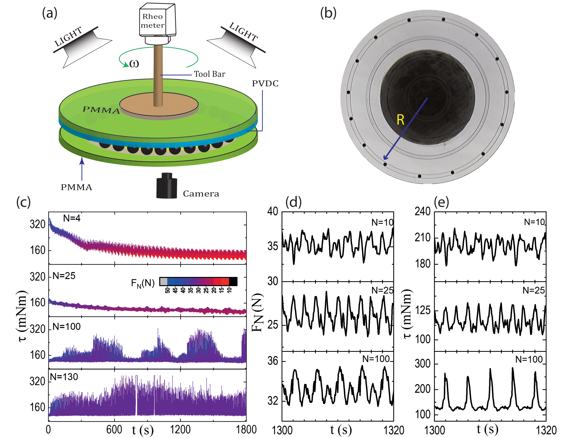
The experimental setup is shown in Fig. 1 (a). A circular plate of transparent Polymethyl methacrylate (PMMA) of $60$ $\rm mm$ radius and $6$ $\rm mm$ thickness is used as the bottom plate into which an annular groove of inner radius $R=47$ $\rm mm$ and width $1.9$ $\rm mm$ is carved. The groove has a depth of $0.6$ $\rm mm$ and it acts as a circular track for the balls to move. $N$ stainless steel balls of diameter $2$ $\rm mm$ are placed on the groove. They are set in motion by rotating the top plate which is coupled to a rheometer (Physica MCR-301) via a shaft. The experiment is performed in two geometries. In the first geometry, the top plate is constructed by attaching a circular transparent Polyvinylidene chloride (PVDC) polymer sheet (see SI supplementary ) of thickness $1$ $\rm mm$ and radius $55$ $\rm mm$ to the bottom surface of a similar-sized circular plate made from PMMA (soft-top and hard-bottom plate geometry). In the second geometry, the top plate is made from PMMA while the bottom plate is made by covering the grooved PMMA plate with a PVDC sheet (hard-top and soft-bottom plate geometry). When the plates are pressed against the balls, the soft PVDC sheet deforms around each ball. The tensile stress developed in the polymer sheet pushes the balls away from each other johnson_1985 (see SI supplementary ) which reduces the inter-ball friction and allows us to run the experiments over a long period of time.

We first describe the experiment in soft-top and hard-bottom plate configuration. Initially, the balls are uniformly distributed on the track and the top plate is made to exert a normal force $F_{N}=30$ $\rm N$ on them. Then the top plate is set to rotate at a uniform angular velocity $\omega=180$ $\rm\deg/s$ while maintaining a constant average gap with the bottom plate. A rheometer is used to monitor both the normal force (resolution $2$ $\rm mN$) and the torque $\tau$ (resolution $1$ $\rm nNm$) acting on the top plate to maintain its set angular velocity at every 100 ms. Additionally, configurations of the balls on the track are continuously imaged at a rate of $3$ frames per second. We perform the experiments by varying the filling fraction of balls, $\rho_{N}=\frac{N}{N_{T}}$, where $N_{T}=150$ is the total number of balls that can be fit on the groove.

The balls can access two motional states - (i) rolling and(ii) sliding kumar2015granular ; ghosh2017geometric ; ghosh2018geometric . They will be referred to as ‘rollers’ and ‘sliders’ respectively. For the ‘rollers’, the top plate moves with a relative velocity $\frac{R\omega}{2}$ with respect to the balls. The ‘sliders’ themselves can be of two types: (i) ‘B-sliders’ - which slide with a velocity $R\omega$ with respect to the bottom plate and are at rest with respect to the top plate and (ii) ‘T-sliders’ - which slide with respect to the top plate and are at rest with respect to the bottom plate. The various spatio-temporal configuration of these ‘rollers’ and ‘sliders’ constitute the internal frictional states of the system and transitions between them generate noise in the friction coefficient. Each of these states is characterized by different frictional forces. We will identify these states from the analysis of the spatio-temporal configurations of the balls later. The force of friction associated with the ‘rollers’ is lower than that associated with the ‘sliders’. In the context of soft-top and hard-bottom plate geometry, the force of friction associated with ‘T-sliders’ is significantly larger than that associated with ‘B-sliders’ (see SI supplementary ).

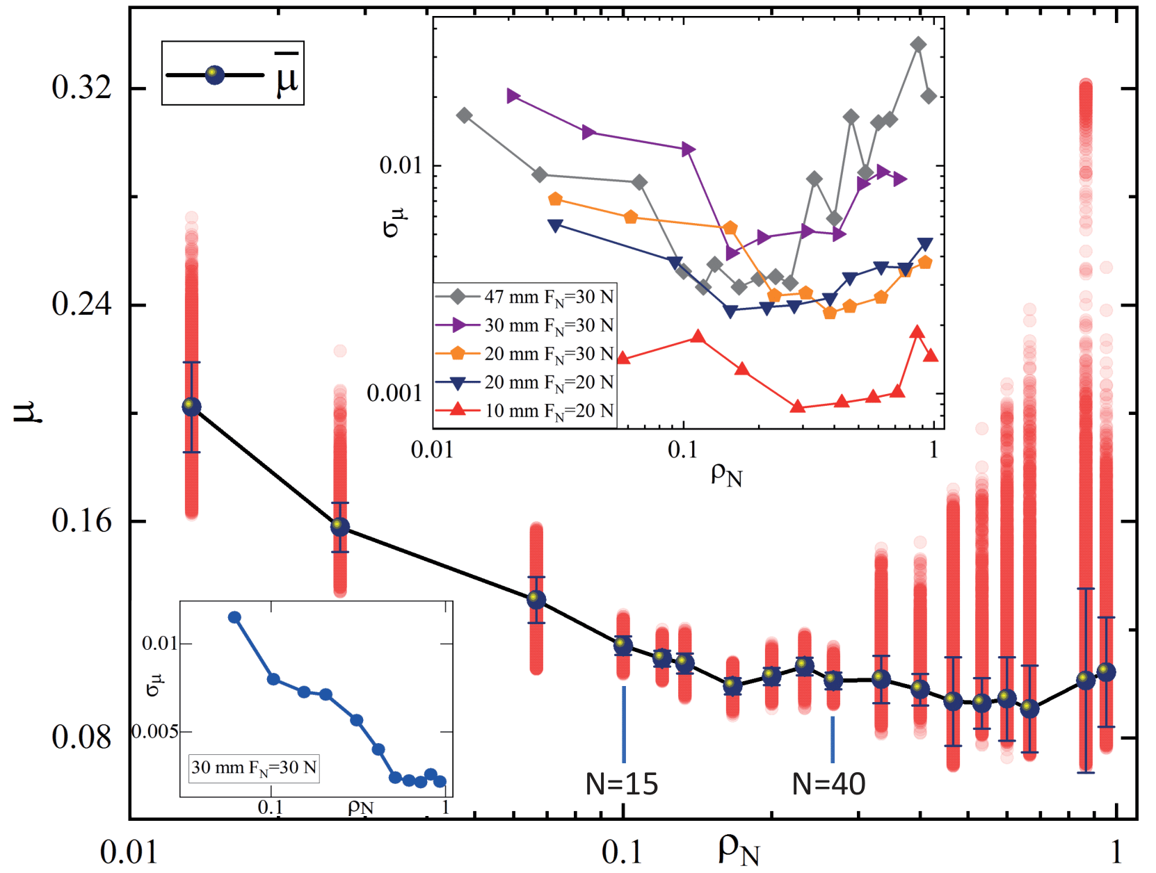
The normal force between the top plate and the balls depends on the extent of deformation made by the balls into the top plate. Due to unintended machining errors and lack of parallelism between the top and bottom plates, the gap height between them has an angular profile (see SI supplementary ). Crests and troughs in the gap profile are not always occupied. As the balls move into/away from these regions, normal force exhibits variation in time which then triggers toggling between the internal frictional states and produces a change in torque [Fig. 1 (d) and (e)]. Figure 2 shows the variation of the coefficient of friction, $\mu=\frac{F_{f}}{F_{N}}=\frac{\tau}{R.F_{N}}$ as a function of $\rho_{N}$, where $F_{f}$ is the friction force acting on the top plate. Clearly, the extent of spread in $\mu$ changes non-monotonically with $\rho_{N}$. The spread in $\mu$ is a measure of the noisiness in the coupling between the plates. Larger the spread, noisier is the coupling. This is particularly evident for small and large $\rho_{N}$. However, for an intermediate-range, $0.1\leq\rho_{N}\leq 0.266$, the extent of variation in $\mu$ is strongly suppressed.

The black dots in Fig. 2 correspond to the measure of the mean value of the friction coefficient $\bar{\mu}$ which decreases with increasing $\rho_{N}$. This drop is related to the concomitant decrease in the fraction of ‘B-sliders’, a feature of the experiment that we will discuss next. We have performed the experiments for different sizes (radius $R$) of the track at different initially applied normal forces and all of these show a dip in the standard deviation in the coefficient of friction, $\sigma_{\mu}$ as a function of $\rho_{N}$ (top right inset of Fig. 2).

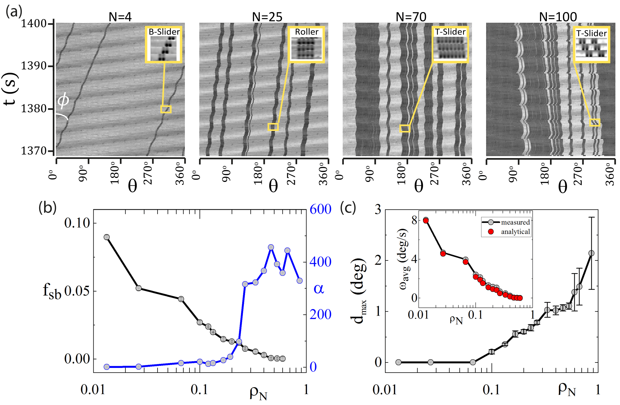
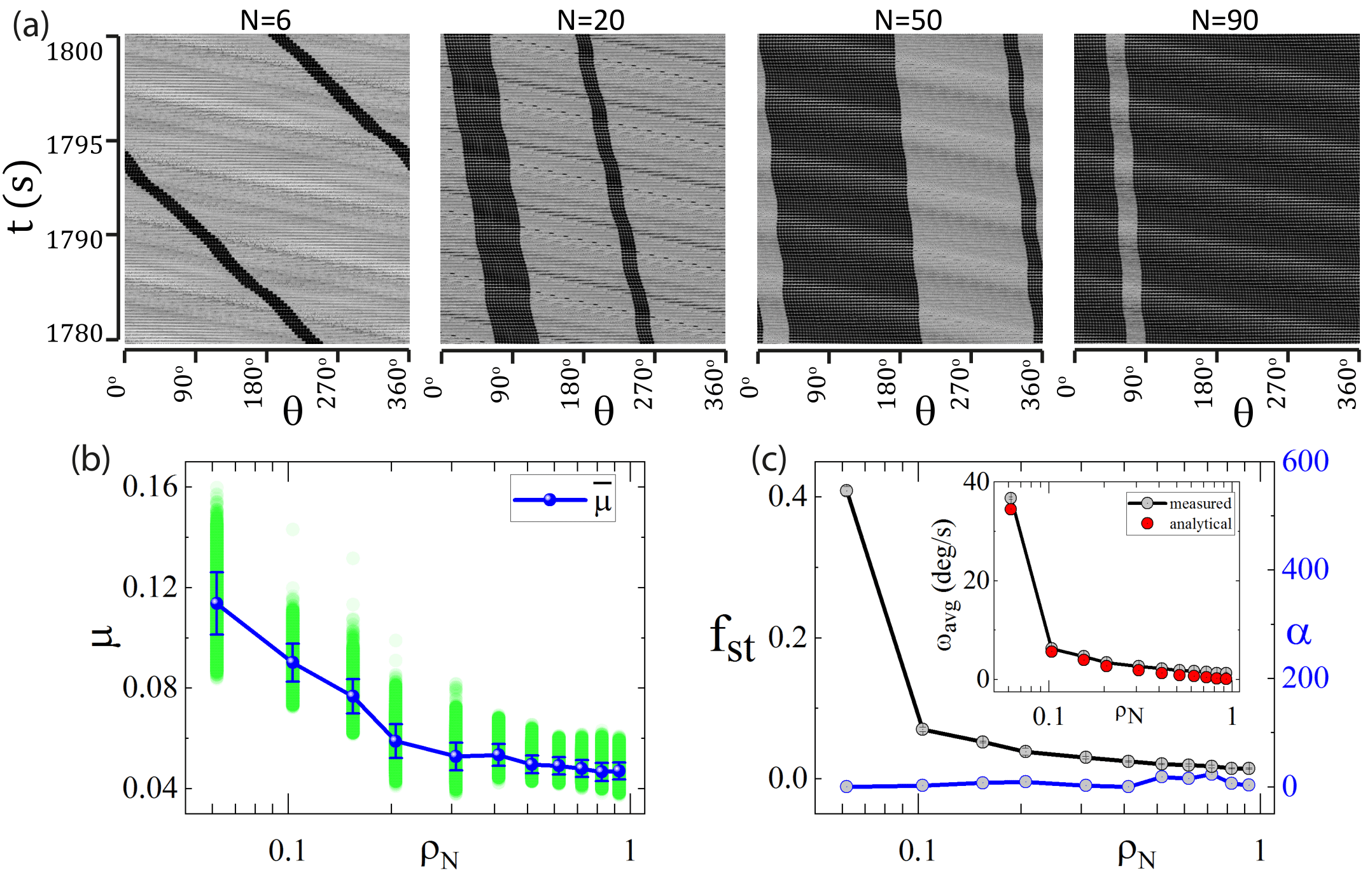
To establish the correlation between the configurations of the balls on the groove and the measurements of friction coefficients, the circular groove is mapped onto a straight line. To figure out the mode of motion of the balls, the pure rolling component of motion is subtracted from the images. These transformed images are referred to be in the ‘R-frame’ of reference. These images are then stacked on top of each other to create a montage [Fig. 3 (a)]. If $\phi$ is the angle of a trajectory with the vertical, then the average velocity can be obtained as $\omega_{avg}=\langle\tan\phi\rangle$. In the ‘R-frame’, ‘rollers’ move parallel to the vertical. For ‘B-sliders’, the trajectory is at an angle $tan^{-1}\left(\frac{\omega}{2}\right)$ with respect to the vertical towards right since the velocity is twice that of pure rolling. While ‘T-sliders’ are at an angle $-tan^{-1}\left(\frac{\omega}{2}\right)$ with respect to the vertical. Therefore, $\omega_{avg}=f_{sb}.\left(\frac{\omega}{2}\right)+f_{r}.0-f_{st}.\left(\frac{\omega}{2}\right)$, where $f_{sb}$, $f_{r}$ and $f_{st}$ are the fractions of time the balls spend as ‘B-sliders’, ‘rollers’ and ‘T-sliders’ respectively and $f_{sb}+f_{r}+f_{st}=1$. It can be observed from Fig. 3 (a) that for small $\rho_{N}$, fraction of ‘B-sliders’ is more. This happens due to large normal force per ball and large frictional grip of the soft top plate on the balls. As $\rho_{N}$ is increased, normal force per ball decreases and balls become more of ‘rollers’. However, with decreasing normal force per ball the extent of deformation in the soft plate reduces which in turn weakens the repulsive interaction between the balls. Thus occasionally balls can touch each other and get jammed momentarily. Hence top plate slip past them and generate ‘T-sliders’. For large $\rho_{N}$ ($N\geq 100$ or $\rho_{N}\geq 0.666$) the system has an overall small sliding component with respect to top plate ($|\tan\phi|\leq 0.1$ $\rm\deg/s$). We have neglected $f_{st}$ while considering the motion of the balls for $\rho_{N}<0.666$. Hence $f_{sb}=\omega_{avg}/\left(\frac{\omega}{2}\right)$ and $f_{r}=1-f_{sb}$. Left $y$ axis in Fig. 3 (b) shows the monotonic decrease of $f_{sb}$ with increasing $\rho_{N}$. Assuming the amplitude of the individual torque signals due to ‘B-sliders’ and ‘rollers’ as $\tau_{sb}$ and $\tau_{r}$ respectively, the rms value of the net torque signal arising from the periodic toggling between ‘B-sliders’ and ‘rollers’ is $\tau_{rms}=\sqrt{\tau_{sb}^{2}D+\tau_{r}^{2}(1-D)}$,where $D=f_{sb}/f_{r}\approx f_{sb}/(1-f_{sb})$ is the duty cycle. Since $\tau_{rms}$ is a monotonically increasing function of $f_{sb}$, the noise in the coupling reduces with decrease in $f_{sb}$ for $\rho_{N}<0.666$.

In the ‘R-frame’ of reference, ‘B-sliders’ contribute to the particle current which decreases with decrease in $f_{sb}$ [grey symbols in inset of Fig. 3 (c)]. The average velocity of the balls in this frame can be calculated analytically by modeling the particle transport in terms of a totally asymmetric simple exclusion process (TASEP) with periodic boundary conditions SCHUTZ20011 ; Kriecherbauer_2010 . This is a reasonably good model if we do not consider the occasional ‘T-sliders’ which are very small even in case of higher $\rho_{N}$. Here we have assumed that for a given $\rho_{N}$, all balls have the same hop rate $p$ which is determined by $f_{sb}$. The average velocity is then given using random sequential update rule as $\omega_{avg}=\left(\frac{\omega}{2}\right).\frac{J}{\rho_{N}}=\left(\frac{\omega}{2}\right).p(1-\rho_{N})$ Rajewsky1998 ; Kanai_2006 ; Kanai_2007 , where $J$ is the average current in the system, $p=f_{sb}$ and $\frac{\omega}{2}$ is the normalization constant. Inset of Fig. 3 (c) shows that measured and analytical average velocities are in good agreement with each other.

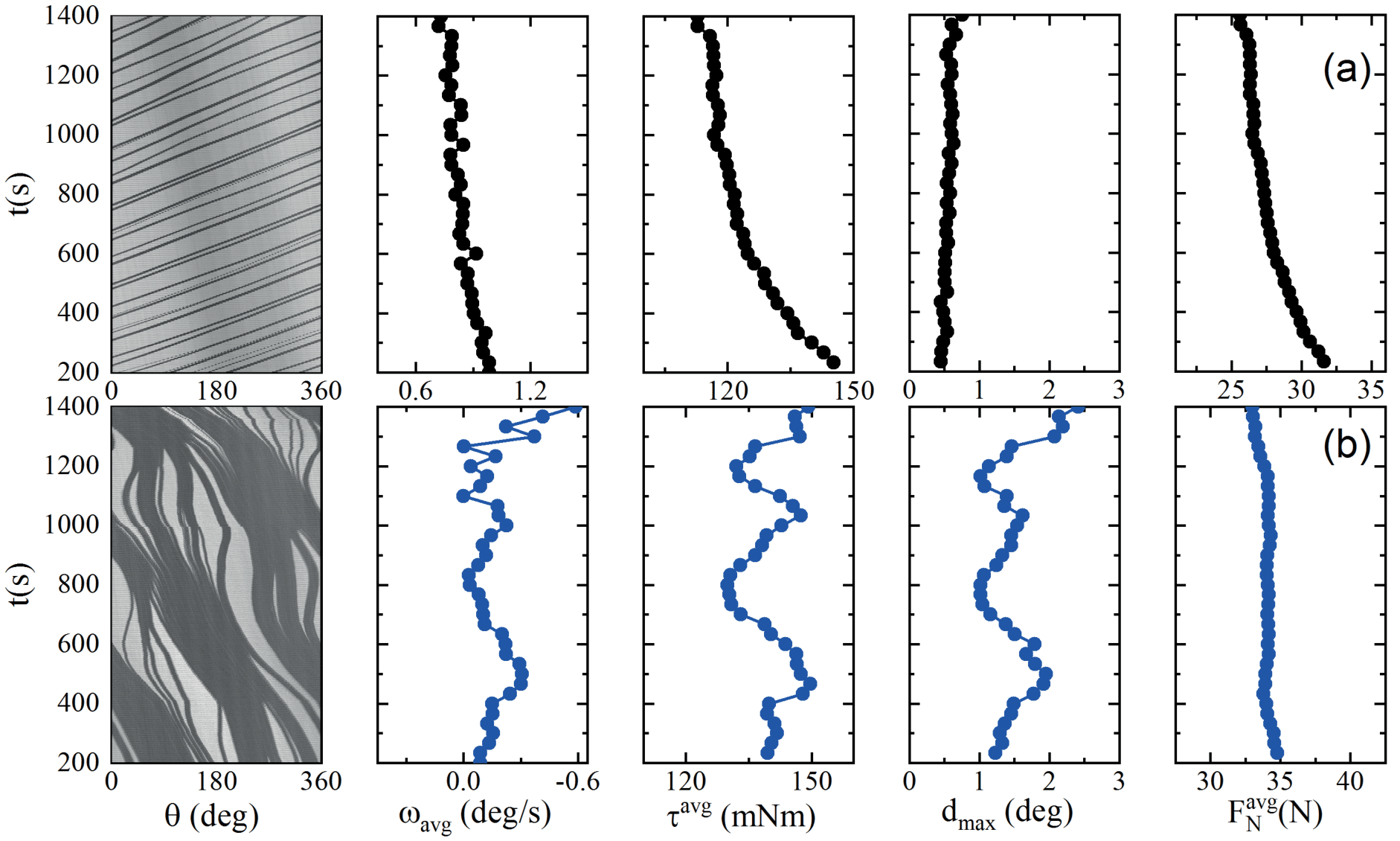
In addition to the monotonic decrease in $f_{sb}$ and $\omega_{avg}$ with $\rho_{N}$, the system also shows a transition from a coherent to an incoherent dynamics as a function of $\rho_{N}$. The fluctuation in the size of the clusters is one measure of such dynamics which is calculated in terms of the quantity $\alpha=\sum_{t}\left|Z_{\rho_{N}}(t)-Z_{\rho_{N}}(t+\delta t)\right|$, where $Z_{\rho_{N}}(t)$ is the total number of clusters in the system at time $t$ and $\delta t=1/3$ s. The data is shown in blue in the right $y$ axis in Fig. 3 (b). For small $\rho_{N}(\leq 0.2)$, the system exhibits coherent dynamics where the clusters do not evolve and all of them keep moving with a nearly constant average velocity [e.g. Fig. 4 (a)]. Whereas for larger $\rho_{N}$, the clusters constantly exchange particles. This results in a considerable variation in average velocity, an example of which is shown in Fig. 4 (b). Note that the trajectories have a negative slope [left panel of Fig. 4 (b)], which corresponds to the top plate slipping with respect to the balls. This happens when there is a transient jam which results in a sudden drop in the mobility of the balls. The slippage events assist the breaking of the clusters by generating elastic disturbances in the top plate. The largest slippage event in a given time interval ($d_{max}$) is strongly correlated with the incoherent dynamics of the cluster coalescence and fragmentation [Fig. 3 (b) and (c)] and the averaged torque ($\tau^{avg}$) in that time interval [third and fourth panel inFig. 4 (b)]. It should be noted from Fig. 4 (b) that the normal force remains mostly silent, i.e., the slowly varying changes in the friction coefficient comes mainly from variations in the torque.

The two above mentioned contributions, i.e., decrease in the sliding of the balls with respect to the bottom plate and increase in the incoherent dynamics of the clusters at large $\rho_{N}$ [Fig. 3 (b) and Fig. 4 (b)] compete with each other to make the noise in $\mu$ to have a non-monotonic dependence on $\rho_{N}$.

In the case of hard-top and soft-bottom plate geometry, the bottom plate exerts a larger frictional grip on the balls and hence ‘B-sliders’ are always absent. In this scenario, the noise in the coupling arises due to the toggling between ‘T-sliders’ and ‘rollers’. With increasing $\rho_{N}$, $f_{st}$ and hence $\sigma_{\mu}$ decreases monotonically with $\rho_{N}$ (bottom left inset of Fig. 2). This is due to the following observation. When $\rho_{N}$ is small, the balls are mainly ‘T-sliders’ as they are held in their place by the large

deformation generated in the soft bottom plate. With increase in $\rho_{N}$, the deformations reduce and the balls begin to roll more (Fig. 5). In the absence of ‘B-sliders’ which slip with respect to the soft plate to generate the elastic disturbances that cause fragmentation of the clusters, the dynamics become coherent for all $\rho_{N}$. The fractions $f_{st}$ and $f_{r}$ can be determined as $f_{st}=\omega_{avg}/\left(\frac{\omega}{2}\right)$ and $f_{r}=1-f_{st}$. In this case, $f_{st}$ decreases monotonically with $\rho_{N}$ (Fig. 5 (c) left y-axis). Toggling between ‘T-sliders’ and ‘rollers’ contributes to the noise in the coupling. The noisiness in the coupling reduces with a decrease in $f_{st}$. Whereas $\alpha$ which is the measure of incoherent dynamics does not change at all [Fig. 5 (c) right y-axis] and all the clusters move with a constant velocity. Hence there is no contribution coming from the exchange dynamics of the clusters to compete against the reduction of noise in $\mu$ due to a decrease in $f_{st}$ with $\rho_{N}$.

In addition, we utilize the recently introduced idea of using lossless data compression PhysRevX.9.011031 to verify the structural correlation in this system. The detailed analysis and results are provided in the supplementary section supplementary .

Frictionally coupled objects when driven tend to get jammed liu1998nonlinear ; bi2011jamming . To unjam the system, it is necessary to periodically inject energy into it. This makes the resulting motion intermittent. In this paper, we demonstrated a route to tune the extent of this intermittency in the third-body friction godet1984third ; godet1990third ; singer1998third ; deng2019simple and via it gain control over the noise in the frictional coupling between two surfaces. In the experiments reported here, steel balls which form the third-body that is sandwiched between a static bottom plate and a rotating top plate, are made to move in single file on a circular track. The noise in the coupling between the plates is measured in terms of the spread in the friction coefficient. Our experimental system is inspired by the mechanical arrangement of a ball bearing. In a conventional ball bearing, balls made from hard materials are sandwiched between the bearing’s inner and outer races. Each ball is held in its place by means of a cage. This ensures that during motion the balls do not collide with each other and get frictionally jammed. Though the collective dynamics of the balls are suppressed in a ball bearing, it can still exhibit noisy dynamics because of the presence of play in its mechanical couplings mevel1993routes ; KAHRAMAN1991469 . In contrast, we do not hold the balls in cages and the noise observed in running our experimental system is related to the collective dynamics of these balls. As a closing remark, we would like to point out that the conventional wisdom that the coefficient of friction is approximately constant for a pair of surfaces ghosh2017geometric can easily be circumvented by harnessing the complexity of the third body interaction forces.

We acknowledge support of the Department of Atomic Energy, Government of India, under Project No. 12-R& DTFR-5.10-0100.

References

- (1) Sclater N, Chironis NP (2001) Mechanisms and mechanical devices sourcebook. (McGraw-Hill New York) Vol. 3.
- (2) Orthwein WC (2004) Clutches and brakes: design and selection. (CRC Press).
- (3) Driving Standards Agency (2005) Driving: The Essential Skills. (The Stationery Office).
- (4) Holmes DG, Lipo TA (2003) Pulse width modulation for power converters: principles and practice. (John Wiley & Sons) Vol. 18.
- (5) Sun J (2012) Pulse-width modulation in Dynamics and control of switched electronic systems. (Springer), pp. 25–61.
- (6) See Supplemental Material for details about experimental setup including materials and methods, characterization of friction, theory of elastic deformation of soft plate, and details of lossless data compression etc.
- (7) Johnson KL, Johnson KL (1987) Contact mechanics. (Cambridge university press).
- (8) Kumar D, Nitsure N, Bhattacharya S, Ghosh S (2015) Granular self-organization by autotuning of friction. Proceedings of the National Academy of Sciences 112(37):11443–11448.
- (9) Ghosh S, Merin A, Nitsure N (2017) On the geometric phenomenology of static friction. Journal of Physics: Condensed Matter 29(35):355001.
- (10) Ghosh S, Merin A, Bhattacharya S, Nitsure N (2018) A geometric framework for dynamics with unilateral constraints and friction, illustrated by an example of self-organized locomotion. Proceedings of the Royal Society A: Mathematical, Physical and Engineering Sciences 474(2212):20170886.
- (11) Schutz G (2000) Exactly solvable models for many-body systems far from equilibrium. Phase transitions and critical phenomena.
- (12) Kriecherbauer T, Krug J (2010) A pedestrian’s view on interacting particle systems, kpz universality and random matrices. Journal of Physics A: Mathematical and Theoretical 43(40):403001.
- (13) Rajewsky N, Santen L, Schadschneider A, Schreckenberg M (1998) The asymmetric exclusion process: Comparison of update procedures. Journal of statistical physics 92(1-2):151–194.
- (14) Kanai M, Nishinari K, Tokihiro T (2006) Exact solution and asymptotic behaviour of the asymmetric simple exclusion process on a ring. Journal of Physics A: Mathematical and General 39(29):9071.
- (15) Kanai M (2007) Exact solution of the zero-range process: fundamental diagram of the corresponding exclusion process. Journal of Physics A: Mathematical and Theoretical 40(26):7127–7138.
- (16) Martiniani S, Chaikin PM, Levine D (2019) Quantifying hidden order out of equilibrium. Phys. Rev. X 9(1):011031.
- (17) Liu AJ, Nagel SR (1998) Nonlinear dynamics: Jamming is not just cool any more. Nature 396(6706):21.
- (18) Bi D, Zhang J, Chakraborty B, Behringer RP (2011) Jamming by shear. Nature 480(7377):355.
- (19) Godet M (1984) The third-body approach: a mechanical view of wear. Wear 100(1-3):437–452.
- (20) Godet M (1990) Third-bodies in tribology. Wear 136(1):29–45.
- (21) Singer IL (1998) How third-body processes affect friction and wear. MRS Bulletin 23(6):37–40.
- (22) Deng F, Tsekenis G, Rubinstein SM (2019) Simple law for third-body friction. Physical review letters 122(13):135503.
- (23) Mevel B, Guyader J (1993) Routes to chaos in ball bearings. Journal of Sound and Vibration 162(3):471–487.
- (24) Kahraman A, Singh R (1991) Non-linear dynamics of a geared rotor-bearing system with multiple clearances. Journal of Sound and Vibration 144(3):469 – 506.