Tuna Nutriment Tracking using Trajectory Mapping in Application to Aquaculture Fish Tank
Abstract
The cost of fish feeding is usually around 40 percent of total production cost. Estimating a state of fishes in a tank and adjusting an amount of nutriments play an important role to manage cost of fish feeding system. Our approach is based on tracking nutriments on videos collected from an active aquaculture fish farm. Tracking approach is applied to acknowledge movement of nutriment to understand more about the fish behavior. Recently, there has been increasing number of researchers focused on developing tracking algorithms to generate more accurate and faster determination of object. Unfortunately, recent studies have shown that efficient and robust tracking of multiple objects with complex relations remain unsolved. Hence, focusing to develop tracking algorithm in aquaculture is more challenging because tracked object has a lot of aquatic variant creatures. By following aforementioned problem, we develop tuna nutriment tracking based on the classical minimum cost problem which consistently performs well in real environment datasets. In evaluation, the proposed method achieved 21.32 pixels and 3.08 pixels for average error distance and standard deviation, respectively. Quantitative evaluation based on the data generated by human annotators shows that the proposed method is valuable for aquaculture fish farm and can be widely applied to real environment datasets.
Index Terms:
Productivity, Fish Feeding, Nutriment, Tracking Algorithm, Real Environment DatasetsI Introduction
Aquaculture is the one of farming type in which aquatic creatures require acceptable environment for living habitat and availability nutriment to increase productivity and sustain healthy growth [1, 2, 3, 4]. Within current requiring acceptable habitat, water quality is also a vital component to enlarge fish fertility rate [3, 4, 5, 6]. Water quality can be obtained by cleaned often and give optimal amount of nutriment. Increasing number of nutriment can affect a lot of foods wasted in the water and quality of water occurs highly polluted. On the other hand, reducing feeding will lead starvation and drop fish quality. So that, management of nutriment delivered is vital component to balance productivity rate [7, 8].
The cost of fish feeding is usually around 40 percent of total production cost [9, 10, 11]. Estimating a state of fishes in a tank and adjusting an amount of nutriments play an important role to manage cost of fish feeding system. It is applied to control the amount of nutriment and realizes the fish behavior in tank. Lately, application to monitor fish behavior has been adopted by a telemetry-based approach [12, 13] and a computer vision(CV)-based approach [14, 15, 16, 17, 18, 19, 20].
A telemetry-based approach is a technique attaching an external transmitter by mounting, or surgical implantation in the peritoneal cavity [12]. Attaching a transmitter in each fish will spend higher cost and its transmitter can only set in large fish. When their fishes had been farmed, attachment will always be given to new fishes. On the other hand, CV-based approach studies are not required complexity analysis such as ripple activity and tracking analysis in which, small number of fishes and small tanks with special environment assist creating result. Tracking approach is applied to acknowledge movement of nutriment to understand more about the fish behavior. Fish behaviors can be obtained by combination between tracking analysis and ripple activity. Then, these fish behaviors can be a decision to start and stop fish feeding machine by understanding of ripple activity after giving several nutriments. By explaining of fish behavior, tracking nutriment is important and it is required to analyze the complexity data in real environment.
Recently, there has been increasing number of researchers focused on developing tracking algorithms to generate more accurate and faster determination of object. Tracking can be represented as a graph problem which can solved by a frame-by-frame [21, 22, 23, 24] or track-by-track [25, 26]. Interpretation of tracking problems with data association mostly uses a graph, where each detection is called as vertex, and each edge is pointing any possible link among them out as object tracked. Data association can be declared as minimum cost problem [27, 28, 29, 30] with learning cost problem [31] or motion pattern maps [32]. Alternative formulations to solve optimization problems is minimum clique problem [33] and lifted multicut problem [34] where its formulations follow body pose layout to obtain estimated model. Recently, efficient and robust tracking of multiple objects with complex relations remain unsolved. Hence, focusing to develop tracking algorithm in aquaculture is more challenging because tracked object has a lot of aquatic variant creatures. By summarizing aforementioned problems, we proposed tuna nutriment tracking based on the classical minimum cost problem [28, 29, 30] where each detection calculates minimum distance among them and creates a trajectory to be tracked line. By collaborating with an active aquaculture fish farm, we develop tuna nutriment tracking using trajectory mapping. A video camera is placed above the boat with a highly disturbance of ocean wave and many dense nutriments. The camera captures between ocean surface and fish feeding machine. After that, videos transfer to a computer for further analysis the behavior of fish.
The aim of this research is tracking approach to acknowledge the behavior of tuna. For next, it can be useful to improve the production profit in fish farms by controlling the amount of nutriment in optimal rate.
To summarize, we make the following contributions:
-
•
We propose tuna nutriment tracking based on trajectory mapping which can perform well as well as human annotator results.
-
•
We propose a new novel small nutriment tracking method with collecting information of leading line into ripple.
-
•
We show significantly improvement result of trajectory mapping in real environment datasets.
II The Proposed Method - Trajectory Mapping
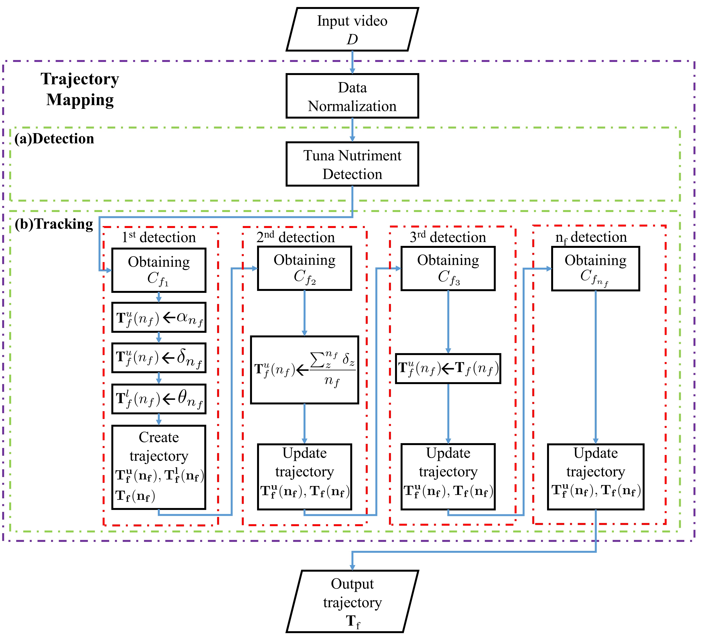
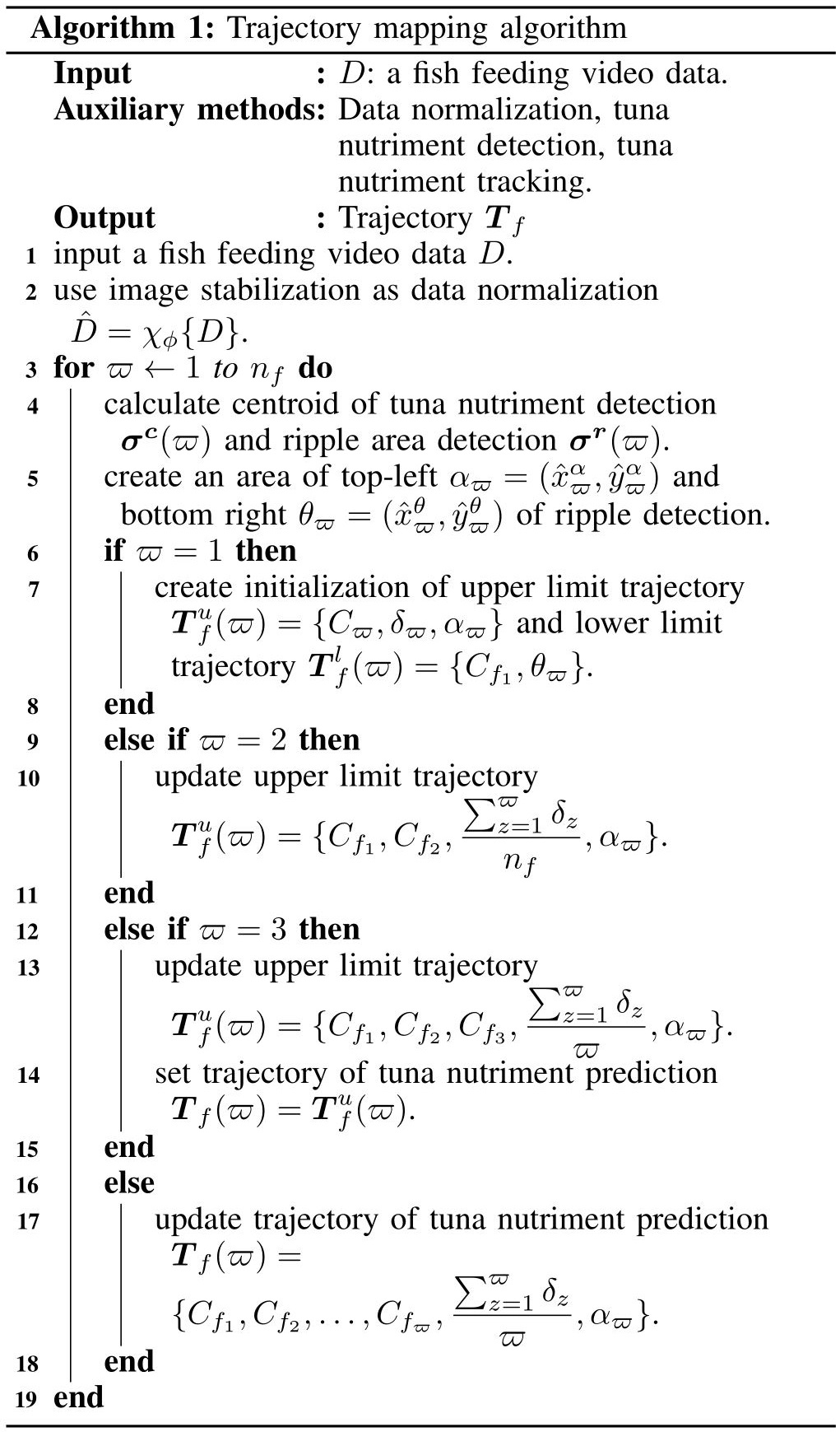
Our formulation is based on the classical minimum cost problem where each detection calculates minimum distance among them and creates a trajectory to be tracked line. In order to provide some background and formally introduce our approach, we start by providing flowchart and algorithm of tuna nutriment tracking. We then explain how the proposed method works to real environment. The proposed trajectory mapping contains a data normalization process, tuna nutriment detection and tuna nutriment tracking. The system flowchart of the proposed method is shown in Fig. 1, and the algorithm of the proposed trajectory mapping is represented in Fig. 2 where and are input video and trajectory of time-ordered tuna nutriment, respectively.
II-A Data Normalization
For data normalization, image stabilization is applied to reduce a hand-held camera and ocean waves. Image stabilization is created by transformation from previous to current frame using optical flow for all frames. [35] accumulates rigid transformation to obtain linked between frame . New rigid transformation in frame can be written as:
| (1) |
where is output video after applied image stabilization and is smoothing radius where the radius is number of frames used for smoothing and defined by 30.
II-B Tuna Nutriment Detection
The idea of tuna nutriment detection is to produce boundary box in each nutriment associated in tracking method. In implementation of tuna nutriment detection, YOLOv3 [36] accumulates bounding box of tuna nutriment prediction by training model with bounding box , , , of ground truth data where , , , and are centroid , centroid , width, and height of bounding box in ground truth data, respectively. and represent the absolute location of the top-left corner of the current grid cell. and are the absolute width and height to the whole image. Bounding box of tuna nutriment prediction can defined as:
| (2) |
where is model followed by [36].
II-C Tuna Nutriment Tracking
In order to represent tracking of tuna nutriment, introducing how to collect set of tuna nutriment prediction corresponding to time-ordered path in the graph is important. We are given as input centroid of tuna nutriment predictions where is the total number of nutriment for all frames of video . Each tuna nutriment prediction is represented by . Definition of a trajectory is denoted as centroid of time-ordered tuna nutriment predictions where is the number of detections formed by trajectory . So that, can be denoted as the total of number of nutriments appearing in every time-ordered trajectory .
II-C1 Problem Statement
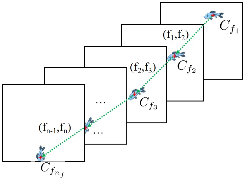
The problem can be represented with an undirected graph , where , and each node denotes a unique detection . The task of dividing the set of tuna nutriment predictions into trajectories can be observed as grouping nodes in graph. Fig. 3 shows that each trajectory in the scene can be mapped into a group of nodes . To produce each , trajectory mapping is applied in next section.
In two-dimensional trajectory, the component of trajectory is divided by horizontal and vertical direction. In vertical direction, acceleration is constant and has quadratic function. Trajectory mapping applies the idea of acceleration and chooses quadratic function as basis.
To produce quadratic function as a result of trajectory , we apply polynomial fitting [37] defined by calculation of to form Vandermonde matrix with columns as results of .
| (3) |
(3) can be inverted directly. To yield the solution vector , it can be defined as:
| (4) |
II-C2 Tuna Nutriment Predictions where as Initialization Point Detection
Tuna nutriment predictions are obtained from every tuna nutriment prediction in around cutting area of . To define cutting area, we use centroid as component of by thresholding in which is defined as:
| (5) |
where is an input parameter and empirically defined as .
Direction of nutriment is calculated by leading nutriment to ripple area around sea levels. We are given a pair set of ripple area detection as time-ordered ripple predictions in number of detections . Each ripple prediction is represented by . We divide component of ripple prediction to be an area of top-left and bottom right of ripple detection by following:
| (6) |
To obtain more feature, we need to know possibly coverage area for possibly nutriment appearing in next frame by creating upper and lower limit trajectory and , respectively. Upper and lower limit trajectory and formed by trajectory are initialized by following:
| (7) |
where is the maximum height of all nutriment detections in . (7) can be simplify by substituting to be:
| (8) |
where .
II-C3 Tuna Nutriment Predictions where
To be a candidate of , we use all tuna nutriment predictions appearing in the inside of area between and . Vector and are produced by calculating and with Vandermonde matrix shown in (3) and (4), respectively. Given is a set of candidate . is defined by the nutriment predictions which have shortest distance denoted by:
| (9) | |||||
where . (9) can be simplify to be;
| (10) |
Updating upper trajectory can be defined as:
| (11) |
II-C4 Tuna Nutriment Predictions where
Minimum requirement for trajectory of quadratic functions must have at least 3 tuna nutriment predictions collected. To produce , (9) is applied using as parameter. Then, updating upper limit trajectory is denoted as follows:
| (12) |
II-C5 Tuna Nutriment Predictions where
To precise accuracy of trajectory , we refine its trajectory by collecting more tuna nutriment prediction . Tuna nutriment prediction is calculated using the nearest nutriment detection in area of with tolerance degree from quadratic function between degree.
To handle losing tuna nutriment prediction, we used previously tuna nutriment prediction by calculating the speed of nutriment in next frame.
| (13) |
where , , and are coefficients of quadratic function formed by trajectory
III Experiment
In this section, we first explain the details of our datasets. We then describe evaluation approach to calculate error rate distance and show quantitative evaluation with various of to discover an optimal value.
III-A Datasets
We report our datasets containing 1 video which has interference of hand-held camera and ocean waves with 419 frames. Each dimension of frame has pixels. Its video sequences are in MOV format with frame rate 30 frames/second. Range size of nutriment is starting from to pixels.
III-B Evaluation Approach
Evaluation approach is defined by measuring minimum euclidean distance based on number of nutriment collected with ground truth . Best trajectory with minimum error rate distance is defined as:
| (14) |
where .
III-C Quantitative Evaluation with various of
| nf | n | Mean (pixels) | Std. Dev. (pixels) | Std. Error (pixels) |
|
|||
|---|---|---|---|---|---|---|---|---|
|
|
|||||||
| 3 | 30 | 185.47 | 93.81 | 17.13 | 150.44 | 220.5 | ||
| 4 | 30 | 78.58 | 33.64 | 6.14 | 66.02 | 91.14 | ||
| 5 | 30 | 25.17 | 13.97 | 2.55 | 19.96 | 30.39 | ||
| 6 | 30 | 21.32 | 3.08 | 0.56 | 20.18 | 22.48 | ||
| 7 | 30 | 35.12 | 19.34 | 3.53 | 27.9 | 42.35 | ||
| 8 | 30 | 32.67 | 4.19 | 0.76 | 31.11 | 34.24 | ||
| 9 | 30 | 44.1 | 13.32 | 2.43 | 39.12 | 49.07 | ||
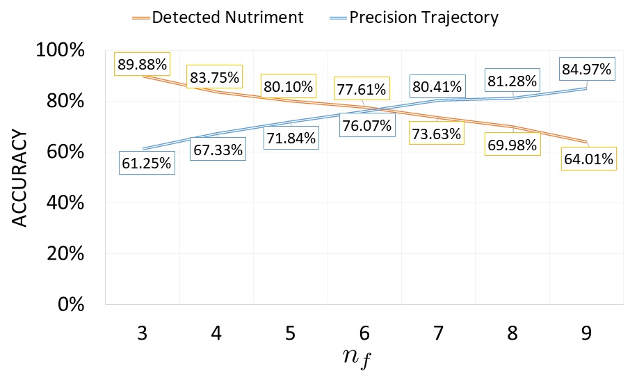
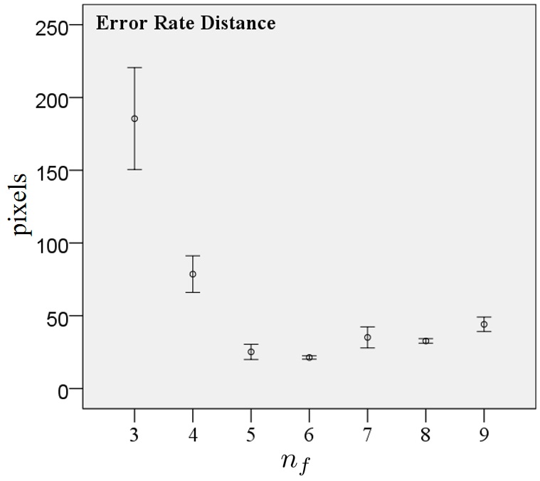
Quantitative evaluation is computed by performance of detected nutriment and precision trajectory showed in Fig. 4. Number of detected nutriment is defined as percentage of detected nutriment divided by ground truth of nutriments appearing in frame. Meanwhile, precision trajectory is computed by total number of nutriments having trajectory leading to ripple area divided by detected nutriment. Fig. 5 and Table I show the confidence interval and statistical analysis of error rate distance in various of . The results show that the optimal value of is in which this parameter produces smallest error rate distance.
IV Result
In this section, we compare proposed method and state-of-the-art benchmark methods on our datasets. After that, we show the figures to explain the advantage of the proposed method and computational time between proposed method and state-of-the-art benchmark methods.
IV-A Evaluation Result
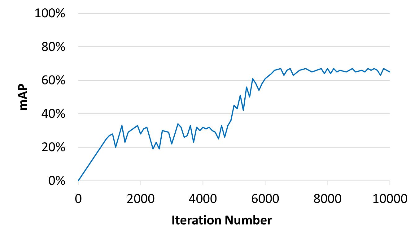
Precision of mAP in object detection is computed by performance YOLOv3 [36] to train our datasets with 10k iterations with pixels for image resizing from pixels. Fig. 6 displays training result of our datasets using YOLOv3 [36] and reaches 67% of maximum mAP with 10k iterations. We also tested proposed methods and state-of-the-art benchmark results. There are many state-of-the-art methods using multiple object tracking (MOT) [38, 39, 40, 41, 42, 43, 44]. These methods perform well using six publicly available datasets on pedestrian detection, MOT and person search provided by [45, 46, 47]. In evaluations, we choose JDE [38] to represent MOT as benchmark method because JDE is very fast and accurate based on re-implementation of faster object detection compared with [39, 40, 41, 42, 43, 44]. We also use SORT [48] as benchmark methods and add our detection model to completely understand performance of tracking method.
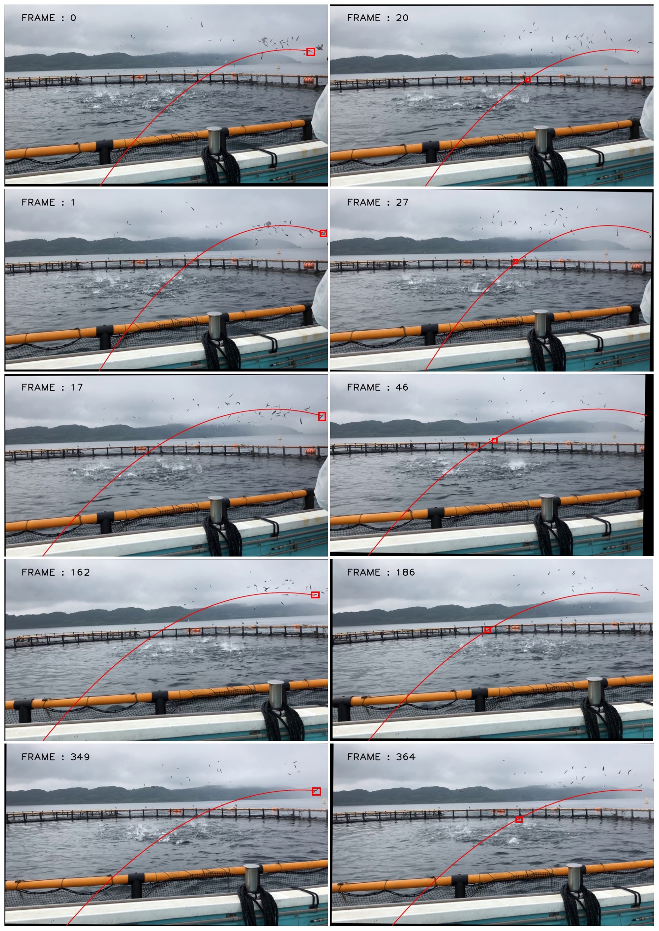
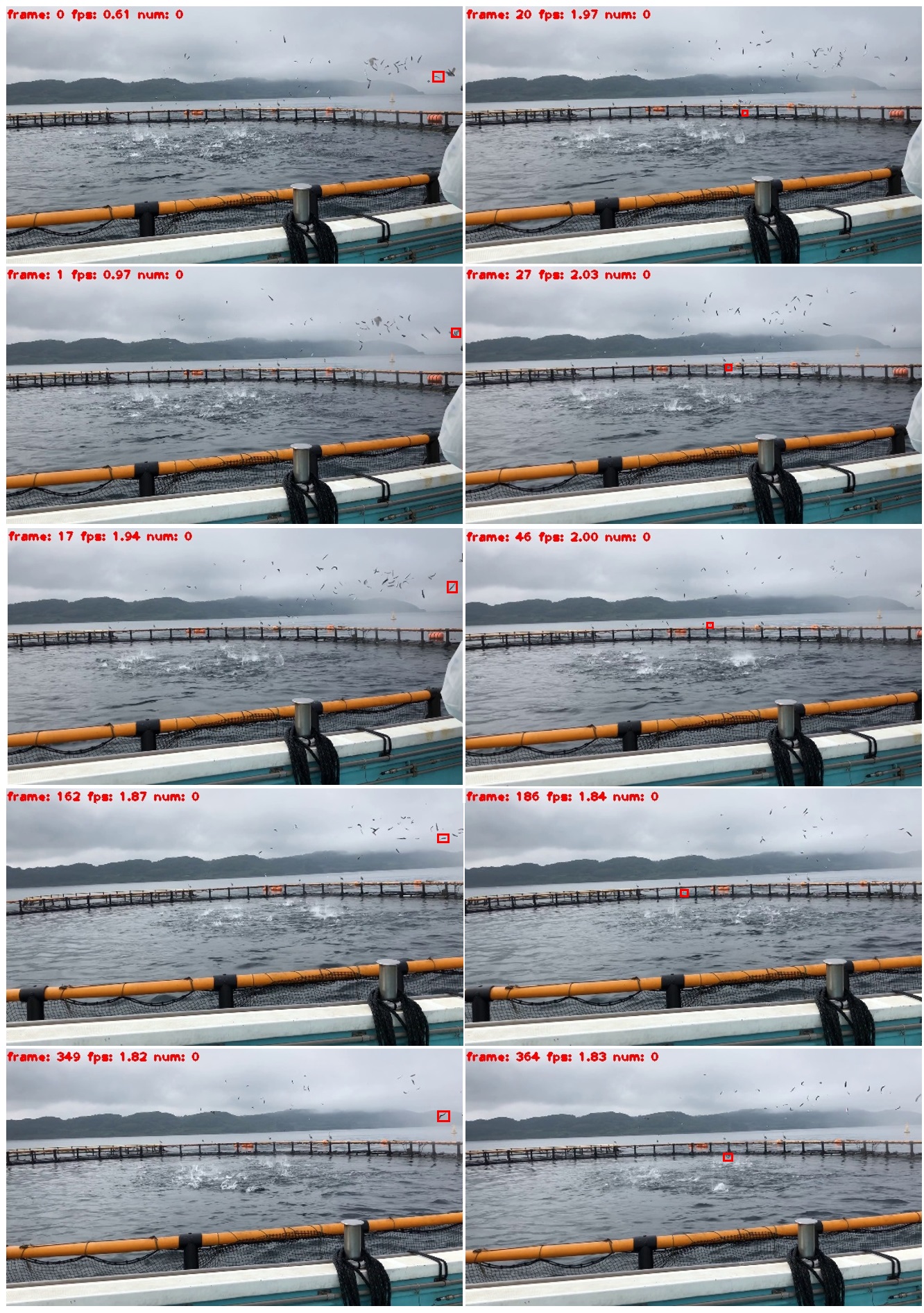
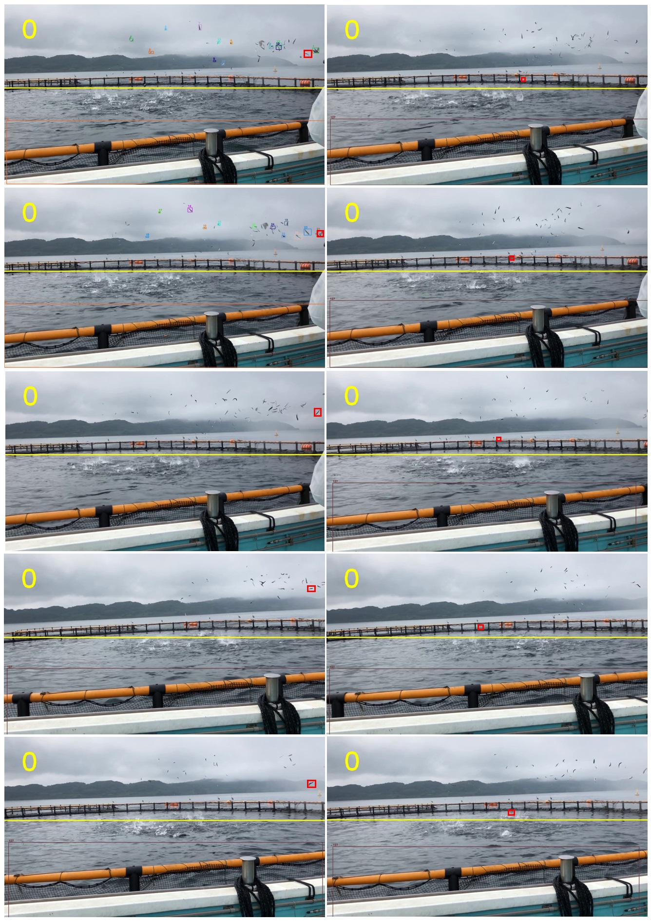
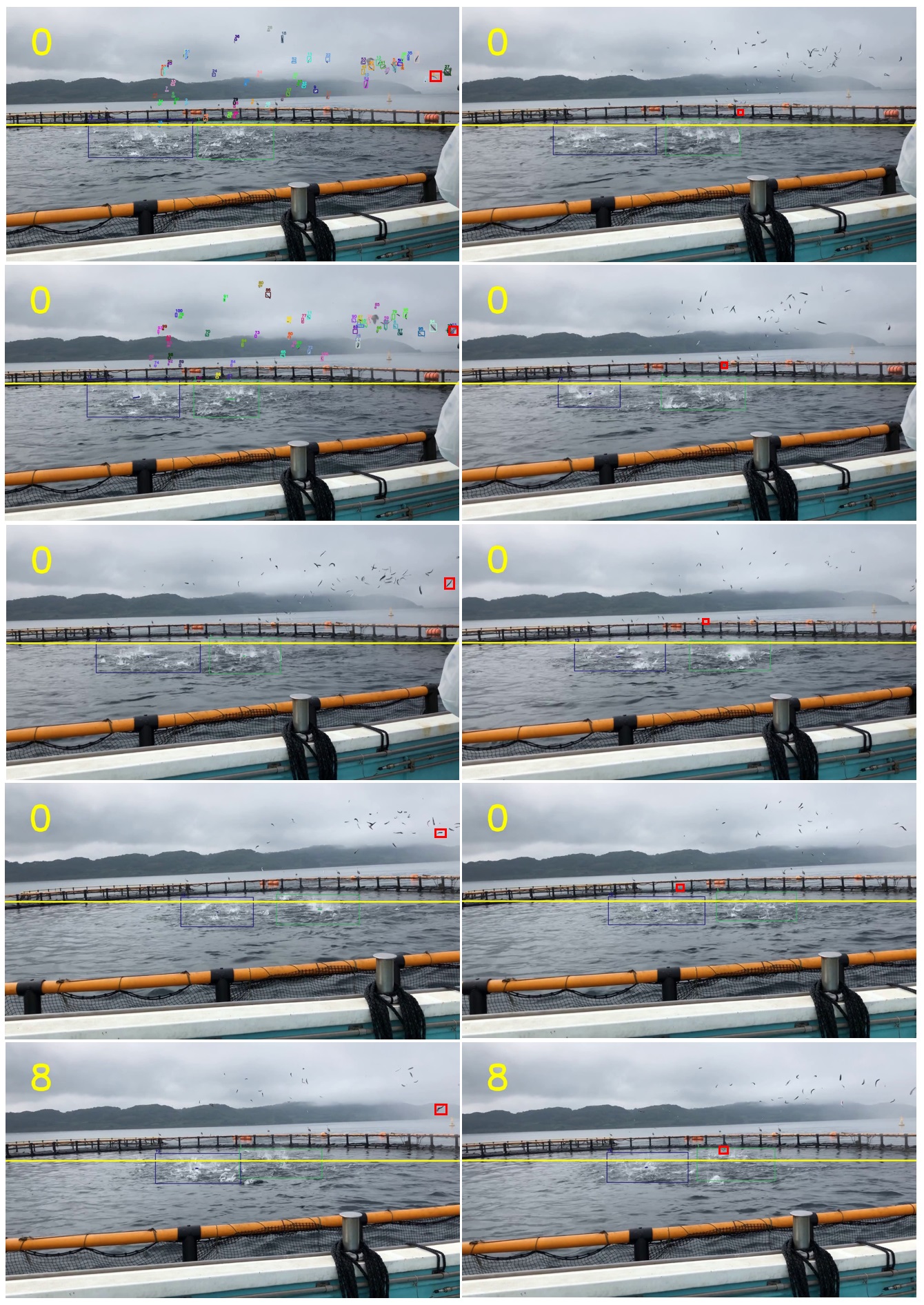
In Fig. 7a, the proposed method is demonstrated to be able to track small nutriment while JDE and SORT with original YOLOv3 and our detection model perform poor (Fig. 7b, 7c, 7d) without tracking results of nutriments even SORT is able to detect some nutriments. By our experiment, the benchmark methods fail to run our datasets because the size of nutriment is too small (maximum size is pixels) and the speed of nutriment is fast (average nutriment movement from start to end node is frames).
IV-B Implementation Details
| Spesification | |||
|---|---|---|---|
| Hardware | CPU | Intel Core i7-9700 CPU @3.00GHz (8 CPUs) | |
| RAM | 16 GB | ||
| GPU | NVIDIA GeForce GTX 745 | ||
| Software | OS | Windows 10 Pro 64-bit | |
| IDE |
|
||
| Language | Python 3.6 64bit | ||
| Methods | N | Mean (fps) | Std. Dev. (fps) | Std. Err. (fps) |
|
|||
|---|---|---|---|---|---|---|---|---|
|
|
|||||||
| Ours | 419 | 1.93 | 0.61 | 0.03 | 1.87 | 1.99 | ||
| JDE | 419 | 1.87 | 0.07 | 0.00 | 1.86 | 1.87 | ||
| YOLOv3 + Sort | 419 | 0.45 | - | - | - | - | ||
|
419 | 0.47 | - | - | - | - | ||
For analysis of the computational complexity and execution time of the proposed methodology, a computational time analysis is conducted using a video with 419 frames. Table II shows the specification of hardware and software for comparison. Table III compares the computation time (in fps) for proposed method, namely trajectory mapping and benchmark approaches: JDE and SORT with original YOLOv3 and our detection model. For average and standard deviation of computational time, we reach and fps, while JDE spends and fps, respectively. SORT only provides average computational time without information of computational time for individual frame. Computational time for both detection model of YOLOv3 and our detection model with SORT performs worst and these benchmark approaches reach fps and , respectively. By analyzing computational complexity, proposed method runs faster than JDE with the different speed is fps.
V Conclusion and Discussion
Tracking approach is the one of features to analyze fish behavior to create a decision to optimize the amount of nutriment. Recent studies have shown that it is possible to track movement objects in entire of frames on video. However, there is no agreement to track multiple small nutriments in the video which has interference of hand-held camera and ocean waves. In this paper, tuna nutriment tracking using trajectory mapping in application to aquaculture fish tank has been presented and demonstrated to be promising for interference video containing multiple small nutriment datasets. We have demonstrated tuna nutriment tracking using trajectory mapping and the method consistently performs well on the interference video with good precision trajectory result. We expect our approach to open the door for future work and to go beyond for feature extraction of ripple activity and focus on integrating tracking approach and ripple activity to be a decision to control fish feeding machine.
References
- [1] F. Fazio, Fish hematology analysis as an important tool of aquaculture: A review. Aquaculture, vol. 500, 237-242, 2019. doi:org/10.1016/j.aquaculture.2018.10.030
- [2] J. Freitas et al., From aquaculture production to consumption: Freshness, safety, traceability and authentication, the four pillars of quality. Aquaculture, vol. 518, 734857, 2019. doi:org/10.1016/j.aquaculture.2019.734857.
- [3] B. Carmen et al., Seagrass meadows improve inflowing water quality in aquaculture ponds. Aquaculture, vol. 528, 735502, 2020. doi:org/10.1016/j.aquaculture.2020.735502.
- [4] W. Liu et al., Characterizing the water quality and microbial communities in different zones of a recirculating aquaculture system using biofloc biofilters. Aquaculture, vol. 529, 735624, 2020. doi:org/10.1016/j.aquaculture.2020.735624.
- [5] U. Farheen et al., Automatic Controlling of Fish Feeding System. International Journal for Research in Applied Science & Engineering Technology (IJRASET), vol. 6, Issue. 7, 362-367, 2018.
- [6] H. Liu et al., Biofloc formation improves water quality and fish yield in a freshwater pond aquaculture system. Aquaculture, vol. 506, 735624, 2019. doi:org/10.1016/j.aquaculture.2019.03.031.
- [7] K. Higuchi et al., Effect of long-term food restriction on reproductive performances in female yellowtail, Seriola quinqueradiata. Aquaculture, vol. 486, 224 - 231, 2018. doi:org/10.1016/j.aquaculture.2017.12.032.
- [8] J.M. Barron et al., Evaluation of effluent waste water from salmonid culture as a potential food and water supply for culturing larval Pacific lamprey Entosphenus tridentatus. Aquaculture, vol. 517, 734791, 2020. doi:org/10.1016/j.aquaculture.2019.734791.
- [9] Y. Atoum et al., Automatic Feeding Control for Dense Aquaculture Fish Tanks. IEEE Signal Process. Lett., vol. 22, 1089-1093, 2015. doi:10.1109/LSP.2014.2385794, 2015.
- [10] A.K. Sabari et al., Smart Fish Feeder. International Journal of Scientific Research in Computer Science, Engineering and Information Technology, vol. 2, Issue. 2, 111-115, 2017.
- [11] P.C. Oostlander et al., Microalgae production cost in aquaculture hatcheries. Aquaculture, vol. 525, 735310, 2020. doi:org/10.1016/j.aquaculture.2020.735310.
- [12] C. J. Bridger and R. K. Booth, The effects of biotelemetry transmitter presence and attachment procedures on fish physiology and behavior. Rev. Fisheries Sci., vol. 11, No. 1, 13–34, 2003.
- [13] S. G. Conti et al., Acoustical monitoring of fish density, behavior, and growth rate in a tank. Aquacult. Eng., vol. 251, No. 2, 314–323, 2006.
- [14] C. Costa et al., Extracting fish size using dual underwater cameras. Aquacult. Eng., vol. 35, No. 3, 218–227, 2006.
- [15] J. Xu et al., Behavioral responses of tilapia (oreochromis niloticus) to acute fluctuations in dissolved oxygen levels as monitored by computer vision. Aquacult. Eng., vol. 35, No. 3, 207–217, 2006.
- [16] L.H. Stien et al., A video analysis procedure for assessing vertical fish distribution in aquaculture tanks. Aquacult. Eng., vol. 37, No. 2, 115–124, 2007.
- [17] B. Zion et al., Real-time underwater sorting of edible fish species. Comput. Electron. Agricult., vol. 56, No. 1, 34–45, 2007.
- [18] S. Duarte et al., Measurement of sole activity by digital image analysis. Aquacult. Eng., vol. 41, No. 1, 22–27, 2009.
- [19] Y. Atoum et al., Automatic Feeding Control for Dense Aquaculture Fish Tanks. IEEE Signal Processing Letters, vol. 22, No. 8, 1089-1093, 2015, doi: 10.1109/LSP.2014.2385794.
- [20] M.A. Adegboye et al., Incorporating Intelligence in Fish Feeding System for Dispensing Feed Based on Fish Feeding Intensity. IEEE Access, vol. 8, 91948-91960, 2020, doi: 10.1109/ACCESS.2020.2994442.
- [21] A. Ess et al., A mobile vision system for robust multi-person tracking. IEEE Conference on Computer Vision and Pattern Recognition (CVPR), 1–8, 2008.
- [22] M. Breitenste et al., Robust tracking-by-detection using a detector confidence particle filter. IEEE International Conference on Computer Vision (ICCV), 1515–1522, 2009.
- [23] S. Pellegrini et al., You’ll never walk alone: modeling social behavior for multi-target tracking. IEEE International Conference on Computer Vision (ICCV), 261–268, 2009.
- [24] T. Ueno et al., Motion-blur-free microscopic video shooting based on frame-by-frame intermittent tracking. IEEE International Conference on Automation Science and Engineering (CASE), 837-842, 2015, doi: 10.1109/CoASE.2015.7294185.
- [25] J. Berclaz et al., Robust people tracking with global trajectory optimization. IEEE Conference on Computer Vision and Pattern Recognition (CVPR), vol. 35, No. 3, 744–750, 2006.
- [26] X. Zhang and E. Izquierdo, Real-Time Multi-Target Multi-Camera Tracking with Spatial-Temporal Information. IEEE Visual Communications and Image Processing (VCIP), 1-4, 2019, doi: 10.1109/VCIP47243.2019.8965845.
- [27] J. Berclaz et al., Multiple object tracking using k-shortest paths optimization. IEEE Transactions on Pattern Analysis and Machine Intelligence (TPAMI), vol. 33, No. 9, 1806–1819, 2011.
- [28] H. Jiang et al., A linear programming approach for multiple object tracking. IEEE Conference on Computer Vision and Pattern Recognition (CVPR), 1–8, 2007.
- [29] L. Zhang et al. Global data association for multi-object tracking using network flows. IEEE Conference on Computer Vision and Pattern Recognition (CVPR), 1–8, 2008.
- [30] H. Pirsiavash et al., Globally optimal greedy algorithms for tracking a variable number of objects. IEEE Conference on Computer Vision and Pattern Recognition (CVPR), 1201–1208, 2011.
- [31] L. Leal-Taixe et al., Learning an image-based motion context for multiple people tracking. IEEE Conference on Computer Vision and Pattern Recognition (CVPR), 2014.
- [32] L. Leal-Taixe et al., Everybody needs somebody: Modeling social and grouping behavior on a linear programming multiple people tracker. IEEE International Conference on Computer Vision (ICCV) Workshops. 1st Workshop on Modeling, Simulation and Visual Analysis of Large Crowds, 2011.
- [33] A. Zamir et al., Gmcp-tracker: Global multi-object tracking using generalized minimum clique graphs. ECCV, 2012.
- [34] S. Tang et al., Multi people tracking with lifted multicut and person re-identification. IEEE Conference on Computer Vision and Pattern Recognition (CVPR), 2017.
- [35] Nghia, Simple video stabilization using OpenCV. http://nghiaho.com/?p=2093, 2010.
- [36] J. Redmon and A. Farhadi, YOLOv3: An Incremental Improvement. CoRR, vol. abs/1804.02767, 2018.
- [37] Weisstein and W. Eric, Least Squares Fitting–Polynomial. From MathWorld–A Wolfram Web Resource, https://mathworld.wolfram.com/LeastSquaresFittingPolynomial.html.
- [38] Z. Wang et al., Towards Real-Time Multi-Object Tracking. CoRR, vol. abs/1909.12605, 2019, http://arxiv.org/abs/1909.12605.
- [39] W. Lin et al., Real-time multi-object tracking with hyper-plane matching. Technical report, , Shanghai Jiao Tong University and ZTE Corp, 2017.
- [40] S. Tang et al., Multiple People Tracking by Lifted Multicut and Person Re-identification. IEEE Conference on Computer Vision and Pattern Recognition (CVPR), Honolulu, HI, 2017, 3701-3710, 2017, doi: 10.1109/CVPR.2017.394.
- [41] Y. Zhang et al., A Simple Baseline for Multi-Object Tracking. CoRR, vol. abs/2004.01888, 2020, https://arxiv.org/abs/2004.01888.
- [42] F. Yu et al., POI: Multiple Object Tracking with High Performance Detection and Appearance Feature. Computer Vision - ECCV 2016 Workshops - Amsterdam, The Netherlands, October 8-10 and 15-16, 2016, Proceedings, Part II, vol. 9914, 36-42, 2016, 10.1007/978-3-319-48881-33.
- [43] M. Babaee et al., A dual CNN-RNN for multiple people tracking. Neurocomputing, vol. 368, 69-83, 2019, 10.1016/j.neucom.2019.08.008.
- [44] B. Pang et al., TubeTK: Adopting Tubes to Track Multi-Object in a One-Step Training Model. CoRR, vol. abs/2006.05683, 2020, https://arxiv.org/abs/2006.05683.
- [45] A. Milan et al., MOT16: A Benchmark for Multi-Object Tracking. CoRR, vol. abs/1603.00831, 2016, http://arxiv.org/abs/1603.00831.
- [46] L. Leal-Taixe et al., MOTChallenge 2015: Towards a Benchmark for Multi-Target Tracking. CoRR, vol. abs/1504.01942, 2015, http://arxiv.org/abs/1504.01942.
- [47] A. Ess et al., Depth and Appearance for Mobile Scene Analysis. IEEE 11th International Conference on Computer Vision, ICCV 2007, Rio de Janeiro, Brazil, October 14-20, 2007, 1-8, 2007, doi:org/10.1109/ICCV.2007.4409092.
- [48] Bewley et al., Simple online and realtime tracking. 2016 IEEE International Conference on Image Processing (ICIP), 3464-3468, 2016, 10.1109/ICIP.2016.7533003.