∎

¹¹institutetext: Zhong-bao Wang, Corresponding author ²²institutetext: 1. Department of Mathematics, Southwest Jiaotong University
Chengdu, Sichuan 611756, China
2. National Engineering Laboratory of Integrated Transportation Big Data Application Technology
Chengdu, Sichuan 611756, China
3. School of Mathematical Sciences, University of Electronic Science and Technology of China
Chengdu, Sichuan, 611731, China
[email protected] ³³institutetext: Zhen-yin Lei ⁴⁴institutetext: 1. Department of Mathematics, Southwest Jiaotong University
Chengdu, Sichuan 611756, China
2. National Engineering Laboratory of Integrated Transportation Big Data Application Technology
Chengdu, Sichuan 611756, China
[email protected] ⁵⁵institutetext: Xin Long ⁶⁶institutetext: 1. Department of Mathematics, Southwest Jiaotong University
Chengdu, Sichuan 611756, China
2. National Engineering Laboratory of Integrated Transportation Big Data Application Technology
Chengdu, Sichuan 611756, China
[email protected] ⁷⁷institutetext: Zhang-you Chen ⁸⁸institutetext: 1. Department of Mathematics, Southwest Jiaotong University
Chengdu, Sichuan 611756, China
2. National Engineering Laboratory of Integrated Transportation Big Data Application Technology
Chengdu, Sichuan 611756, China
[email protected]

Tseng Splitting Method with Double Inertial Steps for Solving Monotone Inclusion Problems

Zhong-bao Wang Zhen-yin Lei Xin Long
Zhang-you Chen

(Received: date / Accepted: date)

Abstract

In this paper, based on double inertial extrapolation steps strategy and relaxed techniques, we introduce a new Tseng splitting method with double inertial extrapolation steps and self-adaptive step sizes for solving monotone inclusion problems in real Hilbert spaces. Under mild and standard assumptions, we establish successively the weak convergence, nonasymptotic $O(\frac{1}{\sqrt{n}})$ convergence rate, strong convergence and linear convergence rate of the proposed algorithm. Finally, several numerical experiments are provided to illustrate the performance and theoretical outcomes of our algorithm.

Keywords Monotone inclusion problem; Tseng splitting method; Double inertial extrapolation steps; Strong and weak convergence; Linear convergence rate

1 Introduction

Let $H$ be a real Hilbert space with the inner product $\left\langle{\cdot,\cdot}\right\rangle$ and the induced norm $\left\|\cdot\right\|$ . The monotone inclusion problem (MIP) is as follows

{\rm find}~{}~{}x^{*}\in H~{}~{}{\rm such~{}that}~{}~{}0\in(A+B)x^{*}.

(1.1)

where $A:H\to H$ is a single mapping and $B:H\to{2^{H}}$ is a multivalued mapping. The solution set is denoted by $\Omega:={(A+B)^{-1}}(0)$ .

The monotone inclusion problem has drawn much attention because it provides a broad unifying frame for variational inequalities, convex minimization problems, split feasibility problems and equilibrium problems, and has been applied to solve several real-world problems from machine learning, signal processing and image restoration, see AB ; BH ; CD ; CW ; DS ; RF ; TYCR .

One of famous methods for solving MIP (1.1) is forward-backward splitting method, which was introduced by Passty PG and Lions et al. LP . This method generates an iterative sequence $\{x_{n}\}$ in following way

{x_{n+1}}={(I+{\lambda_{n}}B)^{-1}}(I-{\lambda_{n}}A){x_{n}}.

(1.2)

where the mapping $A$ is $\frac{1}{L}$ -co-coercive, $B$ is maximal monotone, $I$ is an identity mapping on $H$ and $\lambda_{n}>0$ . The operator $(I-{\lambda_{n}}A)$ is called an forward operator and ${(I+{\lambda_{n}}B)^{-1}}$ is said to be a backward operator.

Tseng TP proposed a modified forward-backward splitting method (also known as Tseng splitting algorithm), whose iterative formula is as follows

\left\{\begin{array}[]{l}{y_{n}}={(I+{\lambda_{n}}B)^{-1}}(I-{\lambda_{n}}A){x_{n}}\\ {x_{n+1}}={y_{n}}-{\lambda_{n}}(A{y_{n}}-A{x_{n}}),\end{array}\right.

(1.3)

where $A$ is $L$ -lipschitz continuous and $\{\lambda_{n}\}\subset(0,1/L)$ . However, the Lipschitz constant of an operator is often unknown or difficult to estimate in nonlinear problems. To overcome this drawback, Cholamjiak et al. CV introduce a relaxed forward-backward splitting method, which uses a simple step-size rule without the prior knowledge of Lipschitz constant of the operator, for solving MIP (1.1) and prove the linear convergence rate of the proposed algorithm.

In recent year, the inertial method was introduced in AF , which can be regarded as a procedure of speeding up the convergence rate of algorithms. Many researchers utilize inertial methods to design algorithm for solving monotone inclusion problems and variational inequalities, see, for example, AB ; CD ; CV ; CH ; CHG ; DQ ; LN ; PTK ; SY ; TD ; YI . To enhance the numerical efficiency, Çopur et al. CHG introduce firstly the double inertial extrapolation steps for solving quasi-variational inequalities in real Hilbert spaces. Combining relaxation techniques with the inertial methods, Cholamjiak et al. CV modify Tseng splitting method to solve MIP (1.1) in real Hilbert spaces. Very recently, incorporating double inertial extrapolation steps and relaxation techniques, Yao et al. YI present a novel subgradients extragradient method to solve variational inequalities, and prove its strong convergence, weak convergence and linear convergence, respectively. However, the linear convergence of YI is obtained under a single inertia rather than double inertias.

This paper devotes to further modifying Tseng splitting method for solving MIP (1.1) in real Hilbert spaces. We obtain successively the weak convergence, nonasymptotic $O(\frac{1}{\sqrt{n}})$ convergence rate, strong convergence and linear convergence rate of the proposed algorithm. Our results obtained in this paper improve the corresponding results in AB ; CV ; CH ; VA ; YI as follows:

$\bullet$ Combining double inertial extrapolation steps strategy and relaxed techniques, we propose a new Tseng splitting method, which include the corresponding methods considered in AB ; CV ; YI as special cases. The two inertial factors in our algorithm are variable sequences, different from the constant inertial factor in AB ; CV ; CH ; YI . Especially, when our algorithm is applied to solving variational inequalities, its some parameters have larger choosing interval than the ones of YI . In addition, one of our inertial factors can be equal to 1, which is not allowed in the single inertial methods CV ; CH , which require that the inertial factor must be strictly less than 1.

$\bullet$ We prove the strong convergence, nonasymptotic $O(\frac{1}{\sqrt{n}})$ convergence rate and linear convergence rate of the proposed algorithm. Note that that the strong convergence does not require to know the modulus of strong monotonicity and the Lipschitz constant in advance. As far as we know, there is no convergence rate results in the literature for methods with double inertial extrapolation steps for solving MIP (1.1) in infinite-dimensional Hilbert spaces.

$\bullet$ Our algorithm use double inertial extrapolation steps to accelerate the speed of the algorithm. The step sizes of our algorithm are updated by a simple calculation without knowing the Lipschitz constant of the underlying operator. Some numerical experiments show that our algorithm has better efficiency than the corresponding algorithms in AB ; CV ; CH ; VA ; YI .

The structure of this article is as follows. In section 2, we recall some essential definitions and results which is relate to this paper. In section 3, we present our algorithm and analyze its weak convergence. In section 4, we establish the strong convergence and the linear convergence rate of our method. In section 5, we present some numerical experiments to demonstrate the performance of our algorithm. We give some concluding remarks in section 6.

2 Preliminaries

In this section, we first give some definitions and results that will be used in this paper. The weak convergence and strong convergence of sequences are denoted by $\rightharpoonup$ and $\to$ , respectively.

Definition 1

The mapping $A:H\rightarrow H$ is called

(i)

pseudomonotone on $H$ if $\langle Ax,y-x\rangle\geq 0$ implies that $\langle Ay,y-x\rangle\geq 0,~{}\forall x,y\in H$ ;
(ii)

monotone on $H$ if

$\langle Ax-Ay,x-y\rangle\geq 0,~{}\forall~{}x,y\in H;$
(iii)

$\mu$ -strongly monotone on $H$ if there exists a positive constant $\mu>0$

$\langle Ax-Ay,x-y\rangle\geq\mu{\left\|{x-y}\right\|^{2}},~{}\forall~{}x,y\in H;$
(iv)

$L$ -lipschitz continuous on $H$ if there exists a scalar $L>0$ satisfying

$\|Ax-Ay\|\leq L\|x-y\|,~{}\forall~{}x,y\in H;$
(v)

$r$ -strongly pseudomonotone on $H$ if there exists a positive constant $r>0$ such that

$\langle Ay,x-y\rangle\geq 0$ implies that $\langle Ax,x-y\rangle\geq r{\left\|{x-y}\right\|^{2}},~{}\forall~{}x,y\in H.$

Definition 2

The graph of $A$ is the set in $H\times H$ defined by

Graph(A):=\{(x,u):x\in H,u\in Ax\}.

Let $C\subset H$ be a nonempty, closed and convex set. The normal cone $N_{C}(x)$ of $C$ at $x$ is represented by

{N_{C}}(x):=\left\{\begin{array}[]{l}\{z\in H:\left\langle{z,y-x}\right\rangle\leq 0,\forall y\in C\},~{}if~{}x\in C,\\ \emptyset,~{}~{}~{}~{}~{}~{}~{}~{}~{}~{}~{}~{}~{}~{}~{}~{}~{}~{}~{}~{}~{}~{}~{}~{}~{}~{}~{}~{}~{}~{}~{}~{}~{}~{}~{}~{}~{}~{}~{}~{}~{}otherwise.\end{array}\right.

The projection of $x\in H$ onto $C$ , denoted by $P_{C}(x)$ , is defined as

{P_{C}}(x):=\arg{\min_{y\in C}}\left\|{x-y}\right\|.

and is has $\left\langle{x-{P_{C}}(x),y-{P_{C}}(x)}\right\rangle\leq 0,\forall y\in C.$
The sequence $\{u_{n}\}$ is $Q$ -linear convergence if there is $q\in(0,1)$ such that $\left\|{{u^{k+1}}-u}\right\|\leq q\left\|{{u^{k}}-u}\right\|$ for all $k$ large enough.

Definition 3

The set-valued mapping $A:H\to{2^{H}}$ is called

(i)

monotone on $H$ if for all $x,y\in H$ , $u\in Ax$ and $v\in Ay$ implies that

$\langle u-v,x-y\rangle\geq 0;$
(ii)

maximal monotone on $H$ if it is monotone and for any $(x,u)\in H\times H,\left\langle{u-v,x-y}\right\rangle\geq 0$ for every $(y,v)\in Graph(A)$ implies that $u\in Ax$ ;
(iii)

$\mu$ -strongly monotone on $H$ if for all $x,y\in H$ , $u\in Ax$ and $v\in Ay$ implies that

$\langle u-v,x-y\rangle\geq\mu{\left\|{x-y}\right\|^{2}},~{}\forall~{}x,y\in H.$

Lemma 1

(MP )Let $\{\varphi_{n}\},\{\delta_{n}\}$ and $\{{\alpha_{n}}\}$ be sequences in $[0,+\infty)$ such that

\varphi_{n+1}\leq\varphi_{n}+{\alpha_{n}}(\varphi_{n}-\varphi_{n-1})+\delta_{n},\forall n\geq 1,\sum\limits_{n=1}^{\infty}{\delta_{n}}<+\infty

and there exists a real number $\alpha$ with $0\leq{\alpha_{n}}\leq\alpha<1$ for all $n\in N$ .Then the following hold :

(i)

$\sum{{}_{n=1}^{+\infty}}{[\varphi_{n}-\varphi_{n-1}]_{+}}<+\infty$ where ${[t]_{+}}:=\max\{t,0\}$ ;
(ii)

there exists ${\varphi^{*}}\in[0,+\infty)$ such that $\mathop{\lim}\limits_{n\to\infty}\varphi_{n}={\varphi^{*}}$ .

Lemma 2

(OZ )Let $C$ be a nonempty set of $H$ and $\{{x_{n}}\}$ be a sequence in $H$ such that the following two conditions hold:

(i)

for every $x\in C,\mathop{\lim}\limits_{n\to\infty}\left\|{{x_{n}}-x}\right\|$ exists;
(ii)

every sequential weak cluster point of $\{{x_{n}}\}$ is in $C$ .

Then $\{{x_{n}}\}$ converges weakly to a point in $C$ .

Lemma 3

TX Let $A:H\to H$ be a maximal monotone mapping and $B:H\to{2^{H}}$ be a Lipschitz continuous and monotone mapping. Then the mapping $A+B$ is a maximal monotone mapping.

Lemma 4

LQ Let $\{a_{n}\}$ and $\{b_{n}\}$ be nonnegative real numbers sequences for which there exists $0\leq q<1$ , so that

a_{n+1}\leq q{a_{n}}+b_{n}~{}~{}for~{}every~{}n\in N.

If $\mathop{\lim}\limits_{n\to\infty}{b_{n}}=0$ , then $\mathop{\lim}\limits_{n\to\infty}{a_{n}}=0$ .

Lemma 5

XH Let $\{{\alpha_{n}}\}$ , $\{a_{n}\}$ , $\{b_{n}\}$ and $\{c_{n}\}$ be nonnegative real numbers sequences and there exists $n_{0}\in N$ such that

{a_{n+1}}\leq(1-{\alpha_{n}}){a_{n}}+{\alpha_{n}}{b_{n}}+{c_{n}}~{}~{}\forall n\geq 1,

where $\{{\alpha_{n}}\}$ , $\{b_{n}\}$ and $\{c_{n}\}$ satisfy the following conditions

(i)

$\{\alpha_{n}\}\subset(0,1)$ and $\sum\limits_{n=0}^{\infty}{{\alpha_{n}}}=\infty;$
(ii)

$\lim{\sup_{n\to\infty}}{b_{n}}\leq 0;$
(iii)

${c_{n}}\geq 0,~{}\forall n\geq 0~{},\sum\limits_{n=1}^{\infty}{{c_{n}}}<\infty$ .

Then $\mathop{\lim}\limits_{n\to\infty}{a_{n}}=0$ .

Lemma 6

GT Let $B:H\to{2^{H}}$ be a set-valued maximal monotone mapping and $A:H\to H$ is a mapping. Define ${T_{\lambda}}:={(I+\lambda B)^{-1}}(I-\lambda A),\lambda>0$ . Then $Fix({T_{\lambda}})={(A+B)^{-1}}0$ .

Lemma 7

(BH ,Corollaty 2.14) For all $x,y\in H$ and $\alpha\in R$ , the following equality holds:

{\left\|{\alpha x+(1-\alpha)y}\right\|^{2}}=\alpha{\left\|x\right\|^{2}}+(1-\alpha){\left\|y\right\|^{2}}-\alpha(1-\alpha){\left\|{x-y}\right\|^{2}}.

3 Weak convergence

In this section, we introduce the Tseng splitting method with double inertial steps to solve MIP (1.1) and discuss convergence and convergence rate of the new algorithm. We firstly give the following conditions.

( $C_{1}$ )

The solution set of the inclusion problem (1.1) is nonempty, that is, $\Omega\neq\emptyset$ .
( $C_{2}$ )

The mappings $A:H\to H$ is $L$ -Lipschitz continuous and monotone and the set-valued mapping $B:H\to{2^{H}}$ is maximal monotone.
( $C_{3}$ )

The real sequences $\{\alpha_{n}\}$ , $\{\beta_{n}\}$ , $\{\beta_{n}\}$ , $\{a_{n}\}$ , $\{p_{n}\}$ and $\{\mu_{n}\}$ satisfy the following conditions
(i)

$0\leq\alpha_{n}\leq 1$ ;
(ii)

$0\leq\beta_{n}\leq\beta_{n+1}\leq\beta<\frac{{3+2\varepsilon-\sqrt{8\varepsilon+17}}}{{2\varepsilon}},\varepsilon\in(1,+\infty)$ ;
(iii)

$0<\theta<\theta_{n}\leq\theta_{n+1}\leq\dfrac{1}{1+\varepsilon},\varepsilon\in(1,+\infty)$ ;
(iv)

${a_{n}}=(1-{\theta_{n}}){\beta_{n}}+{\theta_{n}}{\alpha_{n}}$ is a non-decreasing sequence;
(v)

$\sum\limits_{n=1}^{\infty}{{p_{n}}}<\infty$ and $\mathop{\lim}\limits_{n\to\infty}{\mu_{n}}=0$ .

Remark 1

Note that if $\{\alpha_{n}\}$ is a non-decreasing sequence, $\tilde{\delta}\geq 0$ and $\beta_{n}=\tilde{\delta}\leq\alpha_{1}$ , then the condition ( $C_{3}$ )(iv) holds naturally. In addition, if we choose $\alpha_{n}=\frac{1}{5}+\frac{1}{{6+n}}$ , $\beta_{n}=\frac{1}{6}-\frac{1}{{6+n}}$ and $\theta_{n}=\frac{1}{4}-\frac{1}{{6+n}}$ , then the condition ( $C_{3}$ )(iv) is also true.

Algorithm 3.1

Choose ${x_{0}},{x_{1}}\in H$ , $\mu\in(0,1)$ and $\lambda_{1}>0$

Step 1.

Compute

\begin{array}[]{l}{w_{n}}={x_{n}}+{\alpha_{n}}({x_{n}}-{x_{n-1}})\\ {z_{n}}={x_{n}}+{\beta_{n}}({x_{n}}-{x_{n-1}})\\ {y_{n}}={(I+{\lambda_{n}}B)}^{-1}(I-{\lambda_{n}}A){w_{n}}\end{array}

where

{\lambda_{n+1}}=\left\{\begin{array}[]{l}\min\{\frac{{(\mu_{n}+\mu)\left\|{{w_{n}}-{y_{n}}}\right\|}}{{\left\|{A{w_{n}}-A{y_{n}}}\right\|}},{\lambda_{n}}+p_{n}\},A{w_{n}}\neq A{y_{n}}\\ {\lambda_{n}+p_{n}},\quad\quad\quad\quad\quad\quad\quad\quad{\rm otherwise}.\end{array}\right.

If ${w_{n}}={y_{n}}$ , stop and $y_{n}$ is a solution of the problem (1.1). Otherwise

Step 2.

Compute

${x_{n+1}}=(1-{\theta_{n}}){z_{n}}+{\theta_{n}}({y_{n}}-{\lambda_{n}}(A{y_{n}}-A{w_{n}}))$

Let $n=n+1$ and return to Step 1.

Remark 2

(i)

In our Algorithm 3.1, we can take the inertial factor $\alpha_{n}=1$ . This is not allowed in the corresponding algorithms of CV ; CH , where the only single inertial extrapolation step is considered and the inertia is bounded away from $1$ .
(ii)

In order to get the larger step sizes, being similar to the sequence $\{\theta_{n}\}$ in Algorithm 3.1 of W , the sequence $\{\mu_{n}\}$ is used to relax the parameter $\mu$ . The sequence $\{\theta_{n}\}$ can be called a relaxed parameter sequence, which can often improve numerical efficiency of algorithms, see CV . If $\mu_{n}=0$ , then the step size $\lambda_{n}$ is the same as the one of Algorithm 4.1 in CH . If $\mu_{n}=0$ and $p_{n}=0$ , then the step size $\lambda_{n}$ is the same as the one of Algorithm 3.1 of VA .
(iii)

Note that if $\beta_{n}=0$ , then the condition ( $C_{3}$ )(iii) can be relaxed as $0<\theta<\theta_{n}\leq\theta_{n+1}\leq\dfrac{1}{1+\varepsilon},\varepsilon\in[0,+\infty)$ , which indicates that ${\theta_{n}}=\hat{\theta}$ can equal 1. Setting ${\alpha_{n}}=\alpha$ , ${\theta_{n}}=\hat{\theta}$ , ${\mu_{n}}=0$ and ${\beta_{n}}={p_{n}}=0$ , our algorithm can reduce to Algorithm 2 of CV . In addition, if ${\alpha_{n}}={\theta_{n}}=\alpha$ , ${\mu_{n}}=0$ and ${\beta_{n}}={p_{n}}=0$ , Algorithm 3.1 can reduce to Algorithm 1 of AB .

Lemma 8

The sequences $\{\lambda_{n}\}$ from Algorithm 3.1 is bounded and $\lambda_{n}\in[\min\{\frac{\mu}{L},{\lambda_{1}}\},{\lambda_{1}}+P]$ . Furthermore there exists $\lambda\in[\min\{\frac{\mu}{L},{\lambda_{1}}\},{\lambda_{1}}+P]$ such that $\mathop{\lim}\limits_{n\to\infty}{\lambda_{n}}=\lambda$ , where $P=\sum\limits_{n=1}^{\infty}{{p_{n}}}$ .

Proof

By the definition of $\lambda_{n}$ , if $A{w_{n}}\neq A{y_{n}}$ , we get

\begin{array}[]{l}{\lambda_{n}}\geq\frac{{(\mu+{\mu_{n}})\left\|{w_{n}-y_{n}}\right\|}}{{\left\|{Aw_{n}-Ay_{n}}\right\|}}\geq\frac{{\mu+{\mu_{n}}}}{L}\geq\frac{\mu}{L}.\end{array}

(3.1)

Since $P=\sum\limits_{n=1}^{\infty}{{p_{n}}}$ , we have

\begin{array}[]{l}{\lambda_{n+1}}\leq{\lambda_{n}}+{p_{n}}\leq{\lambda_{1}}+\sum\limits_{n=1}^{\infty}{{p_{n}}}={\lambda_{1}}+P.\end{array}

(3.2)

It implies that $\{\frac{\mu}{L},{\lambda_{1}}\}\leq{\lambda_{n}}\leq{\lambda_{1}}+P$ .
We have

\begin{array}[]{l}{\lambda_{n+1}}-{\lambda_{n}}={[{\lambda_{n+1}}-{\lambda_{n}}]_{+}}-{[{\lambda_{n+1}}-{\lambda_{n}}]_{-}}.\end{array}

(3.3)

Thus

\begin{array}[]{l}{\lambda_{n+1}}-{\lambda_{1}}=\sum\limits_{i=1}^{n}{{{[{\lambda_{i+1}}-{\lambda_{i}}]}_{+}}}-\sum\limits_{i=1}^{n}{{{[{\lambda_{i+1}}-{\lambda_{i}}]}_{-}}}.\end{array}

(3.4)

Since $\{\lambda_{n}\}$ is bounded and $\sum\limits_{n=1}^{\infty}{{{[{\lambda_{n+1}}-{\lambda_{n}}]}_{+}}}\leq\sum\limits_{n=1}^{\infty}{{p_{n}}}<\infty$ , we get $\sum\limits_{n=1}^{\infty}{{{[{\lambda_{n+1}}-{\lambda_{n}}]}_{-}}}$ is convergent. Therefore, there exists $\lambda\in[\min\{\frac{\mu}{L},{\lambda_{1}}\},{\lambda_{1}}+P]$ such that $\mathop{\lim}\limits_{n\to\infty}{\lambda_{n}}=\lambda$ . This proof is completed.

Remark 3

If ${w_{n}}={y_{n}}$ , then ${y_{n}}={(I+{\lambda_{n}}B)}^{-1}(I-{\lambda_{n}}A){y_{n}}$ . By Lemma 6, we know ${y_{n}}\in\Omega$ .

Lemma 9

Suppose that the sequence $\{y_{n}\}$ is generated by Algorithm 3.1. Thus the following assertions hold:

(i)

if the conditions ( $C_{1}$ ) and ( $C_{2}$ ) hold, then

\begin{array}[]{l}{\left\|{{y_{n}}-{\lambda_{n}}(A{y_{n}}-A{w_{n}})-p}\right\|^{2}}\leq{\left\|{{w_{n}}-p}\right\|^{2}}-(1-\frac{{{(\mu+{\mu_{n}})^{2}}{\lambda_{n}}^{2}}}{{{\lambda_{n+1}}^{2}}}){\left\|{{w_{n}}-{y_{n}}}\right\|^{2}},\forall p\in\Omega;\end{array}

(ii)

if the conditions ( $C_{1}$ ) and ( $C_{2}$ ) hold and $A$ or $B$ is $r$ -strongly monotone, then

\begin{array}[]{l}\begin{split}{\left\|{{y_{n}}-{\lambda_{n}}(A{y_{n}}-A{w_{n}})-p}\right\|^{2}}&\leq{\left\|{{w_{n}}-p}\right\|^{2}}-(1-\frac{{{(\mu+{\mu_{n}})^{2}}{\lambda_{n}}^{2}}}{{{\lambda_{n+1}}^{2}}}){\left\|{{w_{n}}-{y_{n}}}\right\|^{2}}\\ &-2r{\lambda_{n}}{\left\|{{y_{n}}-p}\right\|^{2}},\forall p\in\Omega.\end{split}\end{array}

Proof

(i) According to the definition of $\lambda_{n}$ , we have that

\begin{array}[]{c}\begin{split}\left\|{{y_{n}}-{\lambda_{n}}(A{y_{n}}-A{w_{n}})-p}\right\|^{2}&={\left\|{{y_{n}}-p}\right\|^{2}}+{\lambda_{n}}^{2}{\left\|{A{y_{n}}-A{w_{n}}}\right\|^{2}}-2{\lambda_{n}}\left\langle{A{y_{n}}-A{w_{n}},{y_{n}}-p}\right\rangle\\ &\leq{\left\|{{y_{n}}-{w_{n}}}\right\|^{2}}+{\left\|{{w_{n}}-p}\right\|^{2}}+2\left\langle{{y_{n}}-{w_{n}},{w_{n}}-p}\right\rangle\\ &\quad+\frac{{{(\mu+{\mu_{n}})^{2}}{\lambda_{n}}^{2}}}{{{\lambda_{n+1}}^{2}}}{\left\|{{y_{n}}-{w_{n}}}\right\|^{2}}-2{\lambda_{n}}\left\langle{A{y_{n}}-A{w_{n}},{y_{n}}-p}\right\rangle\\ &=(1+\frac{{{(\mu+{\mu_{n}})^{2}}{\lambda_{n}}^{2}}}{{{\lambda_{n+1}}^{2}}}){\left\|{{y_{n}}-{w_{n}}}\right\|^{2}}+{\left\|{{w_{n}}-p}\right\|^{2}}+2\left\langle{{y_{n}}-{w_{n}},{w_{n}}-{y_{n}}}\right\rangle\\ &\quad+2\left\langle{{y_{n}}-{w_{n}},{y_{n}}-p}\right\rangle-2{\lambda_{n}}\left\langle{A{y_{n}}-A{w_{n}},{y_{n}}-p}\right\rangle\\ &=(-1+\frac{{{(\mu+{\mu_{n}})^{2}}{\lambda_{n}}^{2}}}{{{\lambda_{n+1}}^{2}}}){\left\|{{y_{n}}-{w_{n}}}\right\|^{2}}+{\left\|{{w_{n}}-p}\right\|^{2}}\\ &\quad-2\left\langle{{w_{n}}-{y_{n}}-{\lambda_{n}}(A{w_{n}}-A{y_{n}}),{y_{n}}-p}\right\rangle.\end{split}\end{array}

(3.5)

Since ${y_{n}}={(I+{\lambda_{n}}B)^{-1}}(I-{\lambda_{n}}A){w_{n}}$ and $B$ is maximal monotone, we obtain

\frac{{{w_{n}}-{y_{n}}-{\lambda_{n}}A{w_{n}}}}{{{\lambda_{n}}}}\in B{y_{n}}.

(3.6)

Thus

\frac{{{w_{n}}-{y_{n}}-{\lambda_{n}}A{w_{n}}}}{{{\lambda_{n}}}}+A{y_{n}}\in(A+B){y_{n}}.

Since $A:H\to H$ is monotone and $B:H\to{2^{H}}$ is a maximal monotone operator, Lemma 3 implies that $A+B$ is maximal monotone. Since $p\in\Omega$ , $0\in(A+B)p$ and so

\left\langle{\frac{{{w_{n}}-{y_{n}}-{\lambda_{n}}A{w_{n}}}}{{{\lambda_{n}}}}+A{y_{n}}-0,{y_{n}}-p}\right\rangle\geq 0.

Hence

\left\langle{{w_{n}}-{y_{n}}-{\lambda_{n}}(A{w_{n}}-A{y_{n}}),{y_{n}}-p}\right\rangle\geq 0.

(3.7)

Combing (3.5) with (3.7), we get

\begin{array}[]{l}{\left\|{{y_{n}}-{\lambda_{n}}(A{y_{n}}-A{w_{n}})-p}\right\|^{2}}\leq{\left\|{{w_{n}}-p}\right\|^{2}}-(1-\frac{{{(\mu+{\mu_{n}})^{2}}{\lambda_{n}}^{2}}}{{{\lambda_{n+1}}^{2}}}){\left\|{{w_{n}}-{y_{n}}}\right\|^{2}}.\end{array}

(3.8)

The proof of the part (i) is completed.

(ii) Case I $B$ is $r$ -strongly monotone.

Since $p\in\omega$ , we have $0\in(A+B)p$ and thus $-Ap\in Bp$ . Since $B$ is $r$ -strongly monotone, by (3.6), we have

\left\langle{\frac{{{w_{n}}-{y_{n}}-{\lambda_{n}}A{w_{n}}}}{{{\lambda_{n}}}}+Ap,{y_{n}}-p}\right\rangle\geq r{\left\|{{y_{n}}-p}\right\|^{2}}.

(3.9)

The monotonicity of $A$ implies that

\left\langle Ay_{n}-Ap,y_{n}-p\right\rangle\geq 0.

(3.10)

Adding together (3.9) and (3.10), we have

\left\langle{\frac{{{w_{n}}-{y_{n}}-{\lambda_{n}}A{w_{n}}}}{{{\lambda_{n}}}}+A{y_{n}},{y_{n}}-p}\right\rangle\geq r{\left\|{{y_{n}}-p}\right\|^{2}},

which implies

\left\langle{{w_{n}}-{y_{n}}-{\lambda_{n}}A{w_{n}}+{\lambda_{n}}A{y_{n}},{y_{n}}-p}\right\rangle\geq r{\lambda_{n}}{\left\|{{y_{n}}-p}\right\|^{2}}.

(3.11)

Utilizing (3.5) and (3.11), we get

\begin{array}[]{l}\begin{split}{\left\|{{y_{n}}-{\lambda_{n}}(A{y_{n}}-A{w_{n}})-p}\right\|^{2}}&\leq{\left\|{{w_{n}}-p}\right\|^{2}}-(1-\frac{{{(\mu+{\mu_{n}})^{2}}{\lambda_{n}}^{2}}}{{{\lambda_{n+1}}^{2}}}){\left\|{{w_{n}}-{y_{n}}}\right\|^{2}}\\ &-2r{\lambda_{n}}{\left\|{{y_{n}}-p}\right\|^{2}}.\end{split}\end{array}

(3.12)

Case II $A$ is $r$ -strongly monotone.

The strong monotonicity of $A$ implies that

\left\langle Ay_{n}-Ap,y_{n}-p\right\rangle\geq r{\left\|{{y_{n}}-p}\right\|^{2}}.

(3.13)

Since $p\in\omega$ , we have $0\in(A+B)p$ and thus $-Ap\in Bp$ . Since $B$ is monotone, by (3.6), we have

\left\langle{\frac{{{w_{n}}-{y_{n}}-{\lambda_{n}}A{w_{n}}}}{{{\lambda_{n}}}}+Ap,{y_{n}}-p}\right\rangle\geq 0.

(3.14)

The rest of proof is the same as in Case I. This completes the proof of Lemma 9.

Lemma 10

Assume that the conditions ( $C_{1}$ ) and ( $C_{2}$ ) hold, and $\{{w_{n}}\}$ and $\{{y_{n}}\}$ are sequences generated by Algorithm 3.1. If $\mathop{\lim}\limits_{n\to\infty}{\left\|{{w_{n}}-{y_{n}}}\right\|}=0$ and ${\{{w_{n}}\}}$ converges weakly to some $z\in H$ , then $z\in\Omega$ .

Proof

Letting $(u,v)\in$ Graph $(A+B)$ , we get $v-Au\in Bu$ . Since $B$ is maximal monotone, by (3.6), we have

\left\langle v-Au-\frac{{{w_{n}}-{y_{n}}-{\lambda_{n}}A{w_{n}}}}{{{\lambda_{n}}}},u-{y_{n}}\right\rangle\geq 0.

(3.15)

This implies that

\begin{array}[]{c}\begin{split}\left\langle v,u-{y_{n}}\right\rangle&\geq\frac{1}{{{\lambda_{n}}}}\left\langle{\lambda_{n}}Au+{w_{n}}-{y_{n}}-{\lambda_{n}}A{w_{n}},u-{y_{n}}\right\rangle\\ &=\frac{1}{{{\lambda_{n}}}}\left\langle{u-{y_{n}},{w_{n}}-{y_{n}}}\right\rangle+\left\langle{u-{y_{n}},Au-A{w_{n}}}\right\rangle\\ &=\frac{1}{{{\lambda_{n}}}}\left\langle{u-{y_{n}},{w_{n}}-{y_{n}}}\right\rangle+\left\langle{u-{y_{n}},Au-A{y_{n}}}\right\rangle+\left\langle{u-{y_{n}},A{y_{n}}-A{w_{n}}}\right\rangle.\end{split}\end{array}

(3.16)

From the Lipschitz continuity and monotonicity of $A$ , it follows that

\begin{array}[]{c}\begin{split}\left\langle{u-{y_{n}},v}\right\rangle&\geq\frac{1}{{{\lambda_{n}}}}\left\langle{u-{y_{n}},{w_{n}}-{y_{n}}}\right\rangle+\left\langle{u-{y_{n}},A{y_{n}}-A{w_{n}}}\right\rangle\\ &\geq\frac{1}{{{\lambda_{n}}}}\left\langle{u-{y_{n}},{w_{n}}-{y_{n}}}\right\rangle-\left\|{u-{y_{n}}}\right\|\left\|{A{y_{n}}-A{w_{n}}}\right\|\\ &\geq\frac{1}{{{\lambda_{n}}}}\left\langle{u-{y_{n}},{w_{n}}-{y_{n}}}\right\rangle-L\left\|{u-{y_{n}}}\right\|\left\|{{y_{n}}-{w_{n}}}\right\|.\end{split}\end{array}

(3.17)

Since $\mathop{\lim}\limits_{n\to\infty}{\left\|{{w_{n}}-{y_{n}}}\right\|}=0$ , by Lemma 8 and (3.17), we have

\left\langle{u-z,v}\right\rangle=\mathop{\lim}\limits_{n\to\infty}\left\langle{u-{w_{n}},v}\right\rangle=\mathop{\lim}\limits_{n\to\infty}\left\langle{u-{y_{n}},v}\right\rangle\geq 0

Since $v\in(A+B)u$ and $A+B$ is maximal monotone, we know $0\in(A+B)z$ , that is, $z\in\Omega$ . This proof is completed.

Theorem 3.1

Assume that the conditions ( $C_{1}$ )-( $C_{3}$ ) hold. Then the sequence $\{{x_{n}}\}$ from Algorithm 3.1 converges weakly to some element $p\in\Omega$ .

Proof

By the definition of $x_{n+1}$ and Lemma 7, we have

\begin{array}[]{c}\begin{split}{\left\|{{x_{n+1}}-p}\right\|^{2}}&={\left\|{(1-{\theta_{n}}){z_{n}}+{\theta_{n}}({y_{n}}-{\lambda_{n}}(A{y_{n}}-A{w_{n}}))-p}\right\|^{2}}\\ &=(1-{\theta_{n}}){\left\|{{z_{n}}-p}\right\|^{2}}+{\theta_{n}}{\left\|{{y_{n}}-{\lambda_{n}}(A{y_{n}}-A{w_{n}})-p}\right\|^{2}}\\ &\quad-(1-{\theta_{n}}){\theta_{n}}{\left\|{{z_{n}}-{y_{n}}+{\lambda_{n}}(A{y_{n}}-A{w_{n}})}\right\|^{2}}.\end{split}\end{array}

(3.18)

The definition of $x_{n+1}$ implies that ${y_{n}}-{\lambda_{n}}(A{y_{n}}-A{w_{n}})=\frac{{{x_{n+1}}-(1-{\theta_{n}}){z_{n}}}}{{{\theta_{n}}}}$ . Thus

\begin{array}[]{c}\begin{split}{\left\|{{z_{n}}-{y_{n}}+{\lambda_{n}}(A{y_{n}}-A{w_{n}})}\right\|^{2}}&={\left\|{{z_{n}}-\frac{{{x_{n+1}}-(1-{\theta_{n}}){z_{n}}}}{{{\theta_{n}}}}}\right\|^{2}}\\ &=\frac{1}{{{\theta_{n}^{2}}}}{\left\|{{x_{n+1}}-{z_{n}}}\right\|^{2}}.\end{split}\end{array}

(3.19)

By Lemma 9, we have

{\left\|{{y_{n}}-{\lambda_{n}}(A{y_{n}}-A{w_{n}})-p}\right\|^{2}}\leq{\left\|{{w_{n}}-p}\right\|^{2}}-(1-\frac{{{(\mu+{\mu_{n}})^{2}}{\lambda_{n}}^{2}}}{{{\lambda_{n+1}}^{2}}}){\left\|{{w_{n}}-{y_{n}}}\right\|^{2}},\forall p\in\Omega.

(3.20)

Substituting (3.19) and (3.20) into (3.18), we get

\begin{split}{\left\|{{x_{n+1}}-p}\right\|^{2}}&\leq(1-{\theta_{n}}){\left\|{{z_{n}}-p}\right\|^{2}}+{\theta_{n}}{\left\|{{w_{n}}-p}\right\|^{2}}-{\theta_{n}}(1-\frac{{{(\mu+{\mu_{n}})^{2}}{\lambda_{n}}^{2}}}{{{\lambda_{n+1}}^{2}}})\left\|{{w_{n}}-{y_{n}}}\right\|^{2}\\ &\quad-\frac{{1-{\theta_{n}}}}{{{\theta_{n}}}}{\left\|{{x_{n+1}}-{z_{n}}}\right\|^{2}}.\end{split}

(3.21)

Lemma 8 and the fact $\mathop{\lim}\limits_{n\to\infty}{\mu_{n}}=0$ imply that $\mathop{\lim}\limits_{n\to\infty}1-\frac{{{(\mu+{\mu_{n}})^{2}}{\lambda_{n}}^{2}}}{{{\lambda_{n+1}}^{2}}}=1-{\mu^{2}}>0$ . Thus there exists a positive integer $N\geq 1$ such that

{\theta_{n}}(1-\frac{{{(\mu+{\mu_{n}})^{2}}{\lambda_{n}}^{2}}}{{{\lambda_{n+1}}^{2}}})\left\|{{w_{n}}-{y_{n}}}\right\|^{2}\geq 0,~{}\forall~{}n\geq N.

Thanks to (3.21), we have

\left\|{{x_{n+1}}-p}\right\|^{2}\leq(1-{\theta_{n}}){\left\|{{z_{n}}-p}\right\|^{2}}+{\theta_{n}}{\left\|{{w_{n}}-p}\right\|^{2}}-\frac{{1-{\theta_{n}}}}{{{\theta_{n}}}}{\left\|{{x_{n+1}}-{z_{n}}}\right\|^{2}},~{}\forall~{}n\geq N.

(3.22)

By the definition of $z_{n}$ and Lemma 7, we obtain

\begin{array}[]{c}\begin{split}{\left\|{{z_{n}}-p}\right\|^{2}}&={\left\|{{x_{n}}+{\beta_{n}}({x_{n}}-{x_{n-1}})-p}\right\|^{2}}\\ &={\left\|{(1+{\beta_{n}})({x_{n}}-p)-{\beta_{n}}({x_{n-1}}-p)}\right\|^{2}}\\ &=(1+{\beta_{n}}){\left\|{{x_{n}}-p}\right\|^{2}}-{\beta_{n}}{\left\|{{x_{n-1}}-p}\right\|^{2}}+{\beta_{n}}(1+{\beta_{n}}){\left\|{{x_{n}}-{x_{n-1}}}\right\|^{2}}.\end{split}\end{array}

(3.23)

From the definition of $w_{n}$ and Lemma 7, it follows that

{\left\|{{w_{n}}-p}\right\|^{2}}=(1+{\alpha_{n}}){\left\|{{x_{n}}-p}\right\|^{2}}-{\alpha_{n}}{\left\|{{x_{n-1}}-p}\right\|^{2}}+{\alpha_{n}}(1+{\alpha_{n}}){\left\|{{x_{n}}-{x_{n-1}}}\right\|^{2}}.

(3.24)

The definition of $z_{n}$ means that

\begin{array}[]{c}\begin{split}{\left\|{{x_{n+1}}-{z_{n}}}\right\|^{2}}&={\left\|{{x_{n+1}}-{x_{n}}-{\beta_{n}}({x_{n}}-{x_{n-1}})}\right\|^{2}}\\ &\geq{\left\|{{x_{n+1}}-{x_{n}}}\right\|^{2}}+{\beta_{n}}^{2}{\left\|{{x_{n}}-{x_{n-1}}}\right\|^{2}}-2{\beta_{n}}\left\|{{x_{n+1}}-{x_{n}}}\right\|\left\|{{x_{n}}-{x_{n-1}}}\right\|\\ &\geq(1-{\beta_{n}}){\left\|{{x_{n+1}}-{x_{n}}}\right\|^{2}}+({\beta_{n}}^{2}-{\beta_{n}}){\left\|{{x_{n}}-{x_{n-1}}}\right\|^{2}}.\end{split}\end{array}

(3.25)

Owing to (3.23), (3.24), (3.25) and (3.22), we know

\begin{split}\left\|{{x_{n+1}}-p}\right\|^{2}&\leq(1-{\theta_{n}})[(1+{\beta_{n}}){\left\|{{x_{n}}-p}\right\|^{2}}-{\beta_{n}}{\left\|{{x_{n-1}}-p}\right\|^{2}}+{\beta_{n}}(1+{\beta_{n}}){\left\|{{x_{n}}-{x_{n-1}}}\right\|^{2}}]\\ &\quad+{\theta_{n}}[(1+{\alpha_{n}}){\left\|{{x_{n}}-p}\right\|^{2}}-{\alpha_{n}}{\left\|{{x_{n-1}}-p}\right\|^{2}}+{\alpha_{n}}(1+{\alpha_{n}}){\left\|{{x_{n}}-{x_{n-1}}}\right\|^{2}}]\\ &\quad-\frac{{1-{\theta_{n}}}}{{{\theta_{n}}}}[(1-{\beta_{n}}){\left\|{{x_{n+1}}-{x_{n}}}\right\|^{2}}+({\beta_{n}}^{2}-{\beta_{n}}){\left\|{{x_{n}}-{x_{n-1}}}\right\|^{2}}]\\ &\leq[1+(1-{\theta_{n}}){\beta_{n}}+{\theta_{n}}{\alpha_{n}}]{\left\|{{x_{n}}-p}\right\|^{2}}-[(1-{\theta_{n}}){\beta_{n}}+{\theta_{n}}{\alpha_{n}}]{\left\|{{x_{n-1}}-p}\right\|^{2}}\\ &\quad+[(1-{\theta_{n}})(1+{\beta_{n}}){\beta_{n}}+{\theta_{n}}(1+{\alpha_{n}}){\alpha_{n}}-\frac{{(1-{\theta_{n}})}}{{{\theta_{n}}}}({\beta_{n}}^{2}-{\beta_{n}})]{\left\|{{x_{n}}-{x_{n-1}}}\right\|^{2}}\\ &\quad-\frac{{(1-{\theta_{n}})}}{{{\theta_{n}}}}(1-{\beta_{n}}){\left\|{{x_{n+1}}-{x_{n}}}\right\|^{2}}\\ &\leq(1+{a_{n}}){\left\|{{x_{n}}-p}\right\|^{2}}-{a_{n}}{\left\|{{x_{n-1}}-p}\right\|^{2}}+{b_{n}}{\left\|{{x_{n}}-{x_{n-1}}}\right\|^{2}}-{c_{n}}{\left\|{{x_{n+1}}-{x_{n}}}\right\|^{2}}.\end{split}

(3.26)

where ${a_{n}}=(1-{\theta_{n}}){\beta_{n}}+{\theta_{n}}{\alpha_{n}}$ , ${b_{n}}:=(1-{\theta_{n}})(1+{\beta_{n}}){\beta_{n}}+{\theta_{n}}(1+{\alpha_{n}}){\alpha_{n}}-\frac{{1-{\theta_{n}}}}{{{\theta_{n}}}}({\beta_{n}}^{2}-{\beta_{n}})$ and ${c_{n}}:=\frac{{1-{\theta_{n}}}}{{{\theta_{n}}}}(1-{\beta_{n}})$ .
Define

{\Gamma_{n}}:={\left\|{{x_{n}}-p}\right\|^{2}}-{a_{n}}{\left\|{{x_{n-1}}-p}\right\|^{2}}+{b_{n}}{\left\|{{x_{n}}-{x_{n-1}}}\right\|^{2}}

Since $\{a_{n}\}$ is non-decreasing, by (3.26), we deduce that

\begin{array}[]{c}\begin{split}{\Gamma_{n+1}}-{\Gamma_{n}}&={\left\|{{x_{n+1}}-p}\right\|^{2}}-(1+{a_{n+1}}){\left\|{{x_{n}}-p}\right\|^{2}}+{a_{n}}{\left\|{{x_{n-1}}-p}\right\|^{2}}\\ &\quad-{b_{n}}{\left\|{{x_{n}}-{x_{n-1}}}\right\|^{2}}+{b_{n+1}}{\left\|{{x_{n+1}}-{x_{n}}}\right\|^{2}}\\ &\leq{\left\|{{x_{n+1}}-p}\right\|^{2}}-(1+{a_{n}}){\left\|{{x_{n}}-p}\right\|^{2}}+{a_{n}}{\left\|{{x_{n-1}}-p}\right\|^{2}}\\ &\quad-{b_{n}}{\left\|{{x_{n}}-{x_{n-1}}}\right\|^{2}}+{b_{n+1}}{\left\|{{x_{n+1}}-{x_{n}}}\right\|^{2}}\\ &\leq-({c_{n}}-{b_{n+1}}){\left\|{{x_{n+1}}-{x_{n}}}\right\|^{2}}.\end{split}\end{array}

(3.27)

The condition ( $C_{3}$ ) means that

\begin{array}[]{c}\begin{split}{c_{n}}-{b_{n+1}}&=\frac{{1-{\theta_{n}}}}{{{\theta_{n}}}}(1-{\beta_{n}})-(1-{\theta_{n+1}})(1+{\beta_{n+1}}){\beta_{n+1}}-{\theta_{n+1}}(1+{\alpha_{n+1}}){\alpha_{n+1}}\\ &\quad+\frac{{1-{\theta_{n+1}}}}{{{\theta_{n+1}}}}({\beta_{n+1}}^{2}-{\beta_{n+1}})\\ &\geq\frac{{1-{\theta_{n+1}}}}{{{\theta_{n+1}}}}(1-2{\beta_{n+1}}+{\beta_{n+1}}^{2})-(1-{\theta_{n+1}})({\beta_{n+1}}+{\beta_{n+1}}^{2})-2{\theta_{n+1}}\\ &\geq\varepsilon(1-2\beta+{\beta^{2}})-\frac{\varepsilon}{{1+\varepsilon}}(\beta+{\beta^{2}})-\frac{2}{{1+\varepsilon}}\\ &=\frac{1}{{1+\varepsilon}}[{\varepsilon^{2}}{\beta^{2}}-(3\varepsilon+2{\varepsilon^{2}})\beta+({\varepsilon^{2}}+\varepsilon-2)].\end{split}\end{array}

(3.28)

Combining (3.27) and (3.28), we infer that

{\Gamma_{n+1}}-{\Gamma_{n}}\leq-\delta{\left\|{{x_{n+1}}-{x_{n}}}\right\|^{2}}.

(3.29)

where $\delta:=\frac{{{\varepsilon^{2}}{\beta^{2}}-(3\varepsilon+2{\varepsilon^{2}})\beta+({\varepsilon^{2}}+\varepsilon-2)}}{{1+\varepsilon}}$ . Since $\beta<\frac{{3+2\varepsilon-\sqrt{8\varepsilon+17}}}{{2\varepsilon}},\varepsilon\in(1,+\infty)$ , we conclude that $\delta>0$ . From (3.29), it follows that

{\Gamma_{n+1}}-{\Gamma_{n}}\leq 0.

Thus the sequence $\{{\Gamma_{n}}\}$ is nonincreasing. The condition ( $C_{3}$ ) implies that $b_{n}>0$ . Thus

\begin{array}[]{c}\begin{split}{\Gamma_{n}}&={\left\|{{x_{n}}-p}\right\|^{2}}-{a_{n}}{\left\|{{x_{n-1}}-p}\right\|^{2}}+{b_{n}}{\left\|{{x_{n}}-{x_{n-1}}}\right\|^{2}}\\ &\geq{\left\|{{x_{n}}-p}\right\|^{2}}-{a_{n}}{\left\|{{x_{n-1}}-p}\right\|^{2}}.\end{split}\end{array}

(3.30)

This implies that

\begin{array}[]{c}\begin{split}{\left\|{{x_{n}}-p}\right\|^{2}}&\leq{a_{n}}{\left\|{{x_{n-1}}-p}\right\|^{2}}+{\Gamma_{n}}\\ &\leq a{\left\|{{x_{n-1}}-p}\right\|^{2}}+{\Gamma_{1}}\\ &\vdots\\ &\leq{a^{n}}{\left\|{{x_{0}}-p}\right\|^{2}}+{\Gamma_{1}}(1+a+\ldots{a^{n-1}})\\ &\leq{a^{n}}{\left\|{{x_{0}}-p}\right\|^{2}}+\frac{{{\Gamma_{1}}}}{{1-a}}.\end{split}\end{array}

(3.31)

where $a:=\frac{{5+2\varepsilon-\sqrt{8\varepsilon+17}}}{{2+2\varepsilon}}<1$ .
By definition of $\{{\Gamma_{n}}\}$ , we have

\begin{array}[]{c}\begin{split}{\Gamma_{n+1}}&={\left\|{{x_{n+1}}-p}\right\|^{2}}-{a_{n+1}}{\left\|{{x_{n}}-p}\right\|^{2}}+{b_{n+1}}{\left\|{{x_{n+1}}-{x_{n}}}\right\|^{2}}\\ &\geq-{a_{n+1}}{\left\|{{x_{n}}-p}\right\|^{2}}.\end{split}\end{array}

(3.32)

According to (3.31) and (3.32), we infer that

-{\Gamma_{n+1}}\leq{a_{n+1}}{\left\|{{x_{n}}-p}\right\|^{2}}\leq a{\left\|{{x_{n}}-p}\right\|^{2}}\leq{a^{n+1}}{\left\|{{x_{0}}-p}\right\|^{2}}+\frac{{a{\Gamma_{1}}}}{{1-a}}.

(3.33)

By (3.33) and (3.29), we get

\begin{array}[]{c}\begin{split}\delta\sum\limits_{k=1}^{n}{{{\left\|{{x_{k+1}}-{x_{k}}}\right\|}^{2}}\leq{\Gamma_{1}}}-{\Gamma_{n+1}}&\leq{a^{n+1}}{\left\|{{x_{0}}-p}\right\|^{2}}+\frac{{{\Gamma_{1}}}}{{1-a}}\\ &\leq{\left\|{{x_{0}}-p}\right\|^{2}}+\frac{{{\Gamma_{1}}}}{{1-a}}.\end{split}\end{array}

(3.34)

This implies

\sum\limits_{k=1}^{\infty}\|x_{k+1}-x_{k}\|^{2}\leq\infty.

(3.35)

Thus

\left\|{{x_{n+1}}-{x_{n}}}\right\|\to 0,n\to\infty.

(3.36)

The definition of $\{{\Gamma_{n}}\}$ implies that

{\left\|{{x_{n+1}}-{w_{n}}}\right\|^{2}}={\left\|{{x_{n+1}}-{x_{n}}}\right\|^{2}}+{\alpha_{n}}{\left\|{{x_{n}}-{x_{n-1}}}\right\|^{2}}-2{\alpha_{n}}\left\langle{{x_{n+1}}-{x_{n}},{x_{n}}-{x_{n-1}}}\right\rangle.

(3.37)

Since $\{\alpha_{n}\}$ is bounded, by (3.37), we obtain

{\left\|{{x_{n+1}}-{w_{n}}}\right\|^{2}}\to 0,n\to\infty.

(3.38)

On the other hand

\left\|{{x_{n}}-{w_{n}}}\right\|\leq\left\|{{x_{n}}-{x_{n+1}}}\right\|+\left\|{{x_{n+1}}-{w_{n}}}\right\|.

(3.39)

From (3.36) and (3.38), it follows that

{\left\|{{x_{n}}-{w_{n}}}\right\|^{2}}\to 0,n\to\infty.

(3.40)

By (3.26), we have

\begin{array}[]{c}\begin{split}{\left\|{{x_{n+1}}-p}\right\|^{2}}&\leq(1+{a_{n}}){\left\|{{x_{n}}-p}\right\|^{2}}-{a_{n}}{\left\|{{x_{n-1}}-p}\right\|^{2}}+{b_{n}}{\left\|{{x_{n}}-{x_{n-1}}}\right\|^{2}}-{c_{n}}{\left\|{{x_{n+1}}-{x_{n}}}\right\|^{2}}\\ &\leq(1+{a_{n}}){\left\|{{x_{n}}-p}\right\|^{2}}-{a_{n}}{\left\|{{x_{n-1}}-p}\right\|^{2}}+{b_{n}}{\left\|{{x_{n}}-{x_{n-1}}}\right\|^{2}}\\ &={\left\|{{x_{n}}-p}\right\|^{2}}+{a_{n}}({\left\|{{x_{n}}-p}\right\|^{2}}-{\left\|{{x_{n-1}}-p}\right\|^{2}})+{b_{n}}{\left\|{{x_{n}}-{x_{n-1}}}\right\|^{2}}.\end{split}\end{array}

(3.41)

Since $0\leq a_{n}<a<1$ and $\{b_{n}\}$ is bounded, by Lemma 1 and (3.35), we know there exists $l\in[0,+\infty)$ such that

\mathop{\lim}\limits_{n\to\infty}{\left\|{{x_{n}}-p}\right\|^{2}}=l.

(3.42)

Then from (3.24), we have

\begin{array}[]{c}\begin{split}{\left\|{{w_{n}}-p}\right\|^{2}}&=(1+{\alpha_{n}}){\left\|{{x_{n}}-p}\right\|^{2}}-{\alpha_{n}}{\left\|{{x_{n-1}}-p}\right\|^{2}}+{\alpha_{n}}(1+{\alpha_{n}}){\left\|{{x_{n}}-{x_{n-1}}}\right\|^{2}}\\ &={\left\|{{x_{n}}-p}\right\|^{2}}+{\alpha_{n}}({\left\|{{x_{n}}-p}\right\|^{2}}-{\left\|{{x_{n-1}}-p}\right\|^{2}})+{\alpha_{n}}(1+{\alpha_{n}}){\left\|{{x_{n}}-{x_{n-1}}}\right\|^{2}}.\end{split}\end{array}

(3.43)

Since $\{{\alpha_{n}}\}$ is bounded, by (3.36) and (3.42), we obtain

\mathop{\lim}\limits_{n\to\infty}{\left\|{{w_{n}}-p}\right\|^{2}}=l.

(3.44)

Utilizing the similar discussion as in obtaining (3.44), we can get

\mathop{\lim}\limits_{n\to\infty}{\left\|{{z_{n}}-p}\right\|^{2}}=l.

(3.45)

Owing to (3.21), we have

\begin{array}[]{c}\begin{split}{\theta_{n}}(1-\frac{{{(\mu+{\mu_{n}})^{2}}{\lambda_{n}}^{2}}}{{{\lambda_{n+1}}^{2}}}){\left\|{{w_{n}}-{y_{n}}}\right\|^{2}}&\leq(1-{\theta_{n}}){\left\|{{z_{n}}-p}\right\|^{2}}+{\theta_{n}}{\left\|{{w_{n}}-p}\right\|^{2}}\\ &\quad-\frac{{(1-{\theta_{n}})}}{{{\theta_{n}}}}{\left\|{{x_{n+1}}-{z_{n}}}\right\|^{2}}-{\left\|{{x_{n+1}}-p}\right\|^{2}}\\ &\leq(1-{\theta_{n}}){\left\|{{z_{n}}-p}\right\|^{2}}+{\theta_{n}}{\left\|{{w_{n}}-p}\right\|^{2}}-{\left\|{{x_{n+1}}-p}\right\|^{2}}.\end{split}\end{array}

(3.46)

Since $0<\theta_{n}<\dfrac{1}{1+\epsilon},\varepsilon\in(1,+\infty)$ and $\mathop{\lim}\limits_{n\to\infty}1-\frac{{{(\mu+{\mu_{n}})^{2}}{\lambda_{n}}^{2}}}{{{\lambda_{n+1}}^{2}}}=1-{\mu^{2}}>0$ , by (3.42) (3.44) and (3.45), we get $\mathop{\lim}\limits_{n\to\infty}\left\|{{w_{n}}-{y_{n}}}\right\|=0.$

Since $\{{x_{n}}\}$ is bounded, we assume that there exists a subsequence $\{{x_{{n_{k}}}}\}$ of $\{{x_{n}}\}$ such that ${x_{{n_{k}}}}\rightharpoonup z\in H$ . The fact $\lim_{n\to\infty}\|{{w_{n}}-{x_{n}}}\|=0$ implies that ${w_{{n_{k}}}}\rightharpoonup z\in H$ . By Lemma 10, we know $z\in\Omega$ . The two assumptions of Lemma 2 are verified. Lemma 2 ensure that the sequence $\{{x_{n}}\}$ converges weakly to $\mu^{*}\in\Omega$ . The proof is completed.

Let $C$ is a nonempty, closed and convex subset of $H$ . If $B=N_{C}$ , then MIP (1.1) reduce to the following variational inequality, denoted by VI $(A,C)$ : find a point $x^{*}\in C$ such that

\langle A(x^{*}),y-x^{*}\rangle\geq 0,~{}\forall~{}y\in C.

Denote the solution set of VI $(A,C)$ by $S$ .

Assumption 3.1

(i)

The solution set of the problem (VI) is nonempty, that is, $S\neq\emptyset$ .
(ii)

The mapping $A:H\to H$ is pseudomonotone, Lipschitz continuous and $A$ satisfies the condition: for any $\{x_{n}\}\subset H$ with $x_{n}\rightharpoonup w^{*}$ , one has $\|Aw^{*}\|\leq\liminf_{n\to\infty}\|Ax_{n}\|.$

Proposition 1

Suppose that $B=N_{C}$ in Algorithm 3.1. Thus the following statements hold:

(i)

if the Assumption 3.1 hold, then

\begin{array}[]{l}{\left\|{{y_{n}}-{\lambda_{n}}(A{y_{n}}-A{w_{n}})-p}\right\|^{2}}\leq{\left\|{{w_{n}}-p}\right\|^{2}}-(1-\frac{{{(\mu+{\mu_{n}})^{2}}{\lambda_{n}}^{2}}}{{{\lambda_{n+1}}^{2}}}){\left\|{{w_{n}}-{y_{n}}}\right\|^{2}},\forall p\in S;\end{array}

(ii)

if the Assumption 3.1 hold and $A$ is $\mu$ -strongly pseudomonotone, then

\begin{array}[]{l}\begin{split}{\left\|{{y_{n}}-{\lambda_{n}}(A{y_{n}}-A{w_{n}})-p}\right\|^{2}}&\leq{\left\|{{w_{n}}-p}\right\|^{2}}-(1-\frac{{{(\mu+{\mu_{n}})^{2}}{\lambda_{n}}^{2}}}{{{\lambda_{n+1}}^{2}}}){\left\|{{w_{n}}-{y_{n}}}\right\|^{2}}\\ &-2\mu{\lambda_{n}}{\left\|{{y_{n}}-p}\right\|^{2}},\forall p\in S.\end{split}\end{array}

Proof

Since $B=N_{C}$ , we know ${y_{n}}={(I+{\lambda_{n}}B)}^{-1}(I-{\lambda_{n}}A){w_{n}}={P_{C}}({w_{n}}-{\lambda_{n}}A{w_{n}})$ . Thus we get

\left\langle{{y_{n}}-{w_{n}}+{\lambda_{n}}A{w_{n}},{y_{n}}-p}\right\rangle\leq 0.

(3.47)

For any given $p\in S$ , $\left\langle{Ap,y_{n}-p}\right\rangle\geq 0.$ Since $A$ is pseudomonotone, we have

\left\langle{Ay_{n},y_{n}-p}\right\rangle\geq 0.

(3.48)

From (3.47) and (3.48), it follows that

\left\langle{{w_{n}}-{y_{n}}-{\lambda_{n}}A{w_{n}}+{\lambda_{n}}A{y_{n}},{y_{n}}-p}\right\rangle\geq 0.

(3.49)

which is just (3.7). The rest of the proof follows the same arguments as in Lemma 9. The proof of the part (i) is completed.

(ii) For any given $p\in S$ , $\left\langle{Ap,y_{n}-p}\right\rangle\geq 0.$ The strong pseudomonotonicity of $A$ implies that

\left\langle Ay_{n},y_{n}-p\right\rangle\geq\mu{\left\|{{y_{n}}-p}\right\|^{2}}.

(3.50)

According to(3.47) and (3.50), we have

\langle w_{n}-y_{n}-\lambda_{n}(Aw_{n}-Ay_{n}),y_{n}-p\rangle\geq\mu\lambda_{n}{\left\|{{y_{n}}-p}\right\|^{2}}.

(3.51)

The rest of proof is the same as in Lemma 9. This completes the proof of Proposition 1.

Proposition 2

Assume that $B=N_{C}$ , the Assumption 3.1 hold, and $\{{w_{n}}\}$ and $\{{y_{n}}\}$ are sequences generated by Algorithm 3.1. If $\mathop{\lim}\limits_{n\to\infty}{\left\|{{w_{n}}-{y_{n}}}\right\|}=0$ and ${\{{w_{n}}\}}$ converges weakly to some $z\in H$ , then $z\in S$ .

Proof

This proof is the same as in Lemma 3.7 of TYCR , and we omit it.

Corollary 1

If $B=N_{C}$ , the conditions ( $C_{3}$ ) and Assumption 3.1 hold, then the sequence $\{{x_{n}}\}$ from Algorithm 3.1 converges weakly to a point $p\in S$ .

Proof

Replacing Lemmas 9 and 10 by Propositions 1 and 2, respectively and using the same proof as in Theorem 3.1, we obtain the desired conclusion.

Remark 4

Compared with Theorem 4.2 of YI , the advantages of Corollary 1 have (i) the sequence $\{\alpha_{n}\}$ may not be non-decreasing; (ii) the sequence $\{\beta_{n}\}$ may not be a constant; (iii) we require $0<\theta<\theta_{n}\leq\theta_{n+1}<\dfrac{1}{1+\epsilon},\varepsilon\in(1,+\infty)$ other than $\varepsilon\in(2,+\infty)$ , which extend the taking value interval of $\theta_{n}$ . From the numerical experiment in Section 5, it can be seen that the larger the values of $\theta_{n}$ , the better the algorithm performs.

Motivated by the Theorem 5.1 of SILD , which may be the first nonasymptotic convergence rate results of inertial projection-type algorithm for solving variational inequalities with monotone mappings, we give the nonasymptotic $O(\frac{1}{\sqrt{n}})$ convergence rate with $``\min_{N\leq i\leq n}"$ for Algorithm 3.1.

Theorem 3.2

Assume that the conditions ( $C_{1}$ )-( $C_{3}$ ) hold, the sequence $\{x_{n}\}$ be generated by Algorithm 3.1 and $[t]_{+}:=max\{t,0\}$ . Then for any $p\in\Omega$ , there exist constants M such that the following estimate holds

\mathop{\min}\limits_{N\leq i\leq n}\left\|{{w_{i}}-{y_{i}}}\right\|\leq{(\frac{{({{\left\|{{x_{N}}-p}\right\|}^{2}}+\frac{a}{{1-a}}{{[{{\left\|{{x_{N}}-p}\right\|}^{2}}-{{\left\|{{x_{N-1}}-p}\right\|}^{2}}]}_{+}}+\frac{{(2+\frac{{1-\theta}}{{4\theta}})M}}{{1-a}})\frac{1}{{\theta(1-\mu)}}}}{{n-N+1}})^{\frac{1}{2}}}.

Proof

{\theta_{n}}(1-\frac{{{(\mu+{\mu_{n}})^{2}}{\lambda_{n}}^{2}}}{{{\lambda_{n+1}}^{2}}})\left\|{{w_{n}}-{y_{n}}}\right\|^{2}\geq\theta_{n}(1-\mu)\left\|{{w_{n}}-{y_{n}}}\right\|^{2},~{}\forall~{}n\geq N.

Thanks to (3.21), we have, for all $n\geq N$

\begin{split}{\left\|{{x_{n+1}}-p}\right\|^{2}}&\leq(1-{\theta_{n}}){\left\|{{z_{n}}-p}\right\|^{2}}+{\theta_{n}}{\left\|{{w_{n}}-p}\right\|^{2}}-{\theta_{n}}(1-\mu)\left\|{{w_{n}}-{y_{n}}}\right\|^{2}-\frac{{1-{\theta_{n}}}}{{{\theta_{n}}}}{\left\|{{x_{n+1}}-{z_{n}}}\right\|^{2}}\\ &\leq(1-{\theta_{n}}){\left\|{{z_{n}}-p}\right\|^{2}}+{\theta_{n}}{\left\|{{w_{n}}-p}\right\|^{2}}-{\theta}(1-\mu)\left\|{{w_{n}}-{y_{n}}}\right\|^{2}-\frac{{1-{\theta_{n}}}}{{{\theta_{n}}}}{\left\|{{x_{n+1}}-{z_{n}}}\right\|^{2}}.\end{split}

(3.52)

Owing to (3.23), (3.24), (3.25) and (3.52), we know, for all $n\geq N$

\begin{split}\left\|{{x_{n+1}}-p}\right\|^{2}&\leq(1-{\theta_{n}})[(1+{\beta_{n}}){\left\|{{x_{n}}-p}\right\|^{2}}-{\beta_{n}}{\left\|{{x_{n-1}}-p}\right\|^{2}}+{\beta_{n}}(1+{\beta_{n}}){\left\|{{x_{n}}-{x_{n-1}}}\right\|^{2}}]\\ &\quad+{\theta_{n}}[(1+{\alpha_{n}}){\left\|{{x_{n}}-p}\right\|^{2}}-{\alpha_{n}}{\left\|{{x_{n-1}}-p}\right\|^{2}}+{\alpha_{n}}(1+{\alpha_{n}}){\left\|{{x_{n}}-{x_{n-1}}}\right\|^{2}}]\\ &\quad-\frac{{1-{\theta_{n}}}}{{{\theta_{n}}}}[(1-{\beta_{n}}){\left\|{{x_{n+1}}-{x_{n}}}\right\|^{2}}+({\beta_{n}}^{2}-{\beta_{n}}){\left\|{{x_{n}}-{x_{n-1}}}\right\|^{2}}]\\ &\quad-{\theta}(1-\mu)\left\|{{w_{n}}-{y_{n}}}\right\|^{2}\\ &\leq[1+(1-{\theta_{n}}){\beta_{n}}+{\theta_{n}}{\alpha_{n}}]{\left\|{{x_{n}}-p}\right\|^{2}}-[(1-{\theta_{n}}){\beta_{n}}+{\theta_{n}}{\alpha_{n}}]{\left\|{{x_{n-1}}-p}\right\|^{2}}\\ &\quad+[(1-{\theta_{n}})(1+{\beta_{n}}){\beta_{n}}+{\theta_{n}}(1+{\alpha_{n}}){\alpha_{n}}-\frac{{(1-{\theta_{n}})}}{{{\theta_{n}}}}({\beta_{n}}^{2}-{\beta_{n}})]{\left\|{{x_{n}}-{x_{n-1}}}\right\|^{2}}\\ &\quad-\frac{{(1-{\theta_{n}})}}{{{\theta_{n}}}}(1-{\beta_{n}}){\left\|{{x_{n+1}}-{x_{n}}}\right\|^{2}}-{\theta}(1-\mu)\left\|{{w_{n}}-{y_{n}}}\right\|^{2}\\ &\leq(1+{a_{n}}){\left\|{{x_{n}}-p}\right\|^{2}}-{a_{n}}{\left\|{{x_{n-1}}-p}\right\|^{2}}+{b_{n}}{\left\|{{x_{n}}-{x_{n-1}}}\right\|^{2}}-{c_{n}}{\left\|{{x_{n+1}}-{x_{n}}}\right\|^{2}}\\ &\quad-{\theta}(1-\mu)\left\|{{w_{n}}-{y_{n}}}\right\|^{2}.\\ &\leq(1+{a_{n}}){\left\|{{x_{n}}-p}\right\|^{2}}-{a_{n}}{\left\|{{x_{n-1}}-p}\right\|^{2}}+{b_{n}}{\left\|{{x_{n}}-{x_{n-1}}}\right\|^{2}}-{\theta}(1-\mu)\left\|{{w_{n}}-{y_{n}}}\right\|^{2}.\end{split}

(3.53)

where $\{a_{n}\}$ , $\{b_{n}\}$ and $\{c_{n}\}$ have the same definitions as in (3.26).

This implies that, for all $n\geq N$

{\theta}(1-\mu)\left\|{{w_{n}}-{y_{n}}}\right\|^{2}\leq{\left\|{{x_{n}}-p}\right\|^{2}}-\left\|{{x_{n+1}}-p}\right\|^{2}+{a_{n}}({\left\|{{x_{n}}-p}\right\|^{2}}-{\left\|{{x_{n-1}}-p}\right\|^{2}})+{b_{n}}{\left\|{{x_{n}}-{x_{n-1}}}\right\|^{2}}.

(3.54)

Let ${\sigma_{n}}={\left\|{{x_{n}}-p}\right\|^{2}},{K_{n}}={\sigma_{n}}-{\sigma_{n-1}}$ and ${\tau_{n}}={b_{n}}{\left\|{{x_{n}}-{x_{n-1}}}\right\|^{2}}$ . We get, for all $n\geq N$

\begin{split}{\theta}(1-\mu)\left\|{{w_{n}}-{y_{n}}}\right\|^{2}&\leq\sigma_{n}-\sigma_{n+1}+a_{n}K_{n}+\tau_{n}\\ &\leq\sigma_{n}-\sigma_{n+1}+a_{n}[K_{n}]_{+}+\tau_{n}\\ &\leq\sigma_{n}-\sigma_{n+1}+a[K_{n}]_{+}+\tau_{n}\\ \end{split}

(3.55)

where $a$ has been defined in (3.31).
In view of (3.35), we have $\sum\limits_{k=1}^{\infty}\|x_{k+1}-x_{k}\|^{2}\leq\infty$ . Thus, there exists a positive constant $M$ such that

\sum\limits_{k=1}^{\infty}\|x_{k+1}-x_{k}\|^{2}\leq M

Therefore,

\begin{split}\sum\limits_{n=1}^{\infty}{{\tau_{n}}}&=\sum\limits_{n=1}^{\infty}{{b_{n}}{{\left\|{{x_{n}}-{x_{n-1}}}\right\|}^{2}}}\\ &=\sum\limits_{n=1}^{\infty}{[(1-{\theta_{n}})(1+{\beta_{n}}){\beta_{n}}+{\theta_{n}}(1+{\alpha_{n}}){\alpha_{n}}+\frac{{1-{\theta_{n}}}}{{{\theta_{n}}}}({\beta_{n}}-{\beta_{n}}^{2})]{{\left\|{{x_{n}}-{x_{n-1}}}\right\|}^{2}}}\\ &\leq\sum\limits_{n=1}^{\infty}{(2+\frac{{1-\theta}}{{4\theta}}){{\left\|{{x_{n}}-{x_{n-1}}}\right\|}^{2}}}\\ &=(2+\frac{{1-\theta}}{{4\theta}})\sum\limits_{n=1}^{\infty}{{{\left\|{{x_{n}}-{x_{n-1}}}\right\|}^{2}}}\\ &\leq(2+\frac{{1-\theta}}{{4\theta}})M={C_{1}}\end{split}

(3.56)

From (3.53), it follows that, for all $n\geq N$

{K_{n+1}}\leq{a_{n}}{K_{n}}+{\tau_{n}}\leq{a_{n}}{[{K_{n}}]_{+}}+{\tau_{n}}.

Thus,

\begin{split}{[{K_{n+1}}]_{+}}&\leq a{[{K_{n}}]_{+}}+{\tau_{n}}\\ &\leq{a^{n-N+1}}{[{K_{n}}]_{+}}+\sum\limits_{j=1}^{n-N+1}{{a^{j-1}}{\tau_{n+1-j}}}.\end{split}

(3.57)

Combining (3.56) and (3.57), we obtain

\begin{split}\sum\limits_{n=N}^{\infty}{{{[{K_{n+1}}]}_{+}}}&\leq\frac{a}{{1-a}}{[{K_{N}}]_{+}}+\frac{1}{{1-a}}\sum\limits_{n=N}^{\infty}{{\tau_{n}}}\\ &\leq\frac{a}{{1-a}}{[{K_{N}}]_{+}}+\frac{{{C_{1}}}}{{1-a}}.\end{split}

(3.58)

From (3.55), it follows that

\begin{split}\theta(1-\mu)\sum\limits_{n=N}^{n}{{{\left\|{{w_{n}}-{y_{n}}}\right\|}^{2}}}&\leq{\sigma_{N}}-\sigma_{{n+1}}+a\sum\limits_{n=N}^{n}{{{[{K_{n}}]}_{+}}}+\sum\limits_{n=N}^{n}{{\tau_{n}}}\\ &\leq{\sigma_{N}}+a({[{K_{N}}]_{+}}+\sum\limits_{n=N}^{n}{{{[{K_{n+1}}]}_{+}}})+\sum\limits_{n=N}^{n}{{\tau_{n}}}\\ &\leq{\sigma_{N}}+a{[{K_{N}}]_{+}}+\frac{{{a^{2}}}}{{1-a}}{[{K_{N}}]_{+}}+\frac{{a{C_{1}}}}{{1-a}}+{C_{1}}\\ &={\sigma_{N}}+\frac{a}{{1-a}}{[{K_{N}}]_{+}}+\frac{{{C_{1}}}}{{1-a}}\\ &={\sigma_{N}}+\frac{a}{{1-a}}{[{K_{N}}]_{+}}+\frac{{(2+\frac{{1-\theta}}{{4\theta}})M}}{{1-a}}.\end{split}

(3.59)

This implies that

\sum\limits_{i=N}^{n}{{{\left\|{{w_{i}}-{y_{i}}}\right\|}^{2}}}\leq({\left\|{{x_{N}}-p}\right\|^{2}}+\frac{a}{{1-a}}{[{\left\|{{x_{N}}-p}\right\|^{2}}-{\left\|{{x_{N-1}}-p}\right\|^{2}}]_{+}}+\frac{{(2+\frac{{1-\theta}}{{4\theta}})M}}{{1-a}})\frac{1}{{\theta(1-\mu)}}.

(3.60)

and thus

\mathop{\min}\limits_{N\leq i\leq n}{\left\|{{w_{i}}-{y_{i}}}\right\|^{2}}\leq\frac{{({{\left\|{{x_{N}}-p}\right\|}^{2}}+\frac{a}{{1-a}}{{[{{\left\|{{x_{N}}-p}\right\|}^{2}}-{{\left\|{{x_{N-1}}-p}\right\|}^{2}}]}_{+}}+\frac{{(2+\frac{{1-\theta}}{{4\theta}})M}}{{1-a}})\frac{1}{{\theta(1-\mu)}}}}{{n-N+1}}.

(3.61)

Since ${[\mathop{\min}\limits_{N\leq i\leq n}{\left\|{{w_{i}}-{y_{i}}}\right\|^{2}}]^{\frac{1}{2}}}=\mathop{\min}\limits_{N\leq i\leq n}\left\|{{w_{i}}-{y_{i}}}\right\|$ , we get

\mathop{\min}\limits_{N\leq i\leq n}\left\|{{w_{i}}-{y_{i}}}\right\|\leq{(\frac{{({{\left\|{{x_{N}}-p}\right\|}^{2}}+\frac{a}{{1-a}}{{[{{\left\|{{x_{N}}-p}\right\|}^{2}}-{{\left\|{{x_{N-1}}-p}\right\|}^{2}}]}_{+}}+\frac{{(2+\frac{{1-\theta}}{{4\theta}})M}}{{1-a}})\frac{1}{{\theta(1-\mu)}}}}{{n-N+1}})^{\frac{1}{2}}}.

(3.62)

This completes the proof.

Remark 5

By Lemma 6 we know ${y_{n}}={w_{n}}$ implies that $y_{n}$ is a solution of MIP. This means that the error estimate given in Theorem 3.2 can be regarded as the convergence rate of Algorithm 3.1.

4 Strong convergence

In this section, we analyse strong convergence and linear convergence of Algorithm 3.1. Firstly, we give the following assumption.

Assumption 4.1

The mapping $A:H\to H$ is $L$ -Lipschitz continuous, $r$ -strongly monotone and the set-valued mapping $B:H\to{2^{H}}$ is maximal monotone or the mapping $A:H\to H$ is $L$ -Lipschitz continuous, monotone and the set-valued mapping $B:H\to{2^{H}}$ is $r$ -strongly monotone.

Theorem 4.1

Assume that the conditions ( $C_{1}$ ),( $C_{3}$ ) and Assumption 4.1 hold. Let $\{{x_{n}}\}$ be a sequence generated by Algorithm 3.1. Then $\{{x_{n}}\}$ converges strongly to some solution $p\in\Omega$ .

Proof

By (3.18) (3.19) and Lemma 9 (ii), we have

\begin{array}[]{c}\begin{split}{\left\|{{x_{n+1}}-p}\right\|^{2}}&\leq(1-{\theta_{n}}){\left\|{{z_{n}}-p}\right\|^{2}}+{\theta_{n}}{\left\|{{w_{n}}-p}\right\|^{2}}-{\theta_{n}}(1-\frac{{{(\mu+{\mu_{n}})^{2}}{\lambda_{n}}^{2}}}{{{\lambda_{n+1}}^{2}}}){\left\|{{w_{n}}-{y_{n}}}\right\|^{2}}\\ &\quad-2{\theta_{n}}r{\lambda_{n}}{\left\|{{y_{n}}-p}\right\|^{2}}-\frac{{(1-{\theta_{n}})}}{{{\theta_{n}}}}{\left\|{{x_{n+1}}-{z_{n}}}\right\|^{2}}\\ &\leq(1-{\theta_{n}}){\left\|{{z_{n}}-p}\right\|^{2}}+{\theta_{n}}{\left\|{{w_{n}}-p}\right\|^{2}}-{\theta_{n}}(1-\frac{{{(\mu+{\mu_{n}})^{2}}{\lambda_{n}}^{2}}}{{{\lambda_{n+1}}^{2}}}){\left\|{{w_{n}}-{y_{n}}}\right\|^{2}}\\ &\quad-2{\theta_{n}}r{\lambda_{n}}{\left\|{{y_{n}}-p}\right\|^{2}}.\end{split}\end{array}

(4.1)

{\theta_{n}}(1-\frac{{{(\mu+{\mu_{n}})^{2}}{\lambda_{n}}^{2}}}{{{\lambda_{n+1}}^{2}}})\left\|{{w_{n}}-{y_{n}}}\right\|^{2}\geq 0,~{}\forall~{}n\geq N.

It follows that from (4.1)

\begin{array}[]{c}\begin{split}{\left\|{{x_{n+1}}-p}\right\|^{2}}&\leq(1-{\theta_{n}}){\left\|{{z_{n}}-p}\right\|^{2}}+{\theta_{n}}{\left\|{{w_{n}}-p}\right\|^{2}}-2{\theta_{n}}r{\lambda_{n}}{\left\|{{y_{n}}-p}\right\|^{2}}\\ &\leq(1-{\theta_{n}}){\left\|{{z_{n}}-p}\right\|^{2}}+{\theta_{n}}{\left\|{{w_{n}}-p}\right\|^{2}}-2\theta r{\lambda_{n}}{\left\|{{y_{n}}-p}\right\|^{2}},~{}\forall n\geq N.\end{split}\end{array}

(4.2)

From Lemma 8, it follows that

\begin{array}[]{c}{\left\|{{x_{n+1}}-p}\right\|^{2}}\leq(1-{\theta_{n}}){\left\|{{z_{n}}-p}\right\|^{2}}+{\theta_{n}}{\left\|{{w_{n}}-p}\right\|^{2}}-2\theta r\lambda^{*}{\left\|{{y_{n}}-p}\right\|^{2}},~{}\forall n\geq N,\end{array}

(4.3)

where $\lambda^{*}=\min\{\frac{\mu}{L},{\lambda_{1}}\}$ .
The definition of $w_{n}$ implies that

\begin{array}[]{c}\begin{split}{\left\|{{w_{n}}-p}\right\|^{2}}&={\left\|{{x_{n}}+{\alpha_{n}}({x_{n}}-{x_{n-1}})-p}\right\|^{2}}\\ &\leq{\left\|{{x_{n}}-p}\right\|^{2}}+{\alpha_{n}}^{2}{\left\|{{x_{n}}-{x_{n-1}}}\right\|^{2}}+2{\alpha_{n}}\left\|{{x_{n}}-p}\right\|\left\|{{x_{n}}-{x_{n-1}}}\right\|.\end{split}\end{array}

(4.4)

By utilizing the definition of $z_{n}$ , we have

\begin{array}[]{c}{\left\|{{z_{n}}-p}\right\|^{2}}\leq{\left\|{{x_{n}}-p}\right\|^{2}}+{\beta_{n}}^{2}{\left\|{{x_{n}}-{x_{n-1}}}\right\|^{2}}+2{\beta_{n}}\left\|{{x_{n}}-p}\right\|\left\|{{x_{n}}-{x_{n-1}}}\right\|.\end{array}

(4.5)

Combining (4.3) (4.4) and (4.5), we obtain

\begin{array}[]{c}\begin{split}{\left\|{{x_{n+1}}-p}\right\|^{2}}&\leq(1-{\theta_{n}})({\left\|{{x_{n}}-p}\right\|^{2}}+{\beta_{n}}^{2}{\left\|{{x_{n}}-{x_{n-1}}}\right\|^{2}}+2{\beta_{n}}\left\|{{x_{n}}-p}\right\|\left\|{{x_{n}}-{x_{n-1}}}\right\|)\\ &\quad+{\theta_{n}}({\left\|{{x_{n}}-p}\right\|^{2}}+{\alpha_{n}}^{2}{\left\|{{x_{n}}-{x_{n-1}}}\right\|^{2}}+2{\alpha_{n}}\left\|{{x_{n}}-p}\right\|\left\|{{x_{n}}-{x_{n-1}}}\right\|)\\ &\quad-2{\theta}\lambda^{*}r{\left\|{{y_{n}}-p}\right\|^{2}}\\ &={\left\|{{x_{n}}-p}\right\|^{2}}+((1-{\theta_{n}}){\beta_{n}}^{2}+{\theta_{n}}{\alpha_{n}}^{2}){\left\|{{x_{n}}-{x_{n-1}}}\right\|^{2}}\\ &\quad+2((1-{\theta_{n}}){\beta_{n}}+{\theta_{n}}{\alpha_{n}})\left\|{{x_{n}}-p}\right\|\left\|{{x_{n}}-{x_{n-1}}}\right\|-2{\theta}\lambda^{*}r{\left\|{{y_{n}}-p}\right\|^{2}},~{}\forall n\geq N.\end{split}\end{array}

(4.6)

In addition,

\begin{array}[]{c}\begin{split}{\left\|{{x_{n}}-p}\right\|^{2}}&\leq 2({\left\|{{x_{n}}-{y_{n}}}\right\|^{2}}+{\left\|{{y_{n}}-p}\right\|^{2}})\\ &\leq 4({\left\|{{x_{n}}-{w_{n}}}\right\|^{2}}+{\left\|{{y_{n}}-{w_{n}}}\right\|^{2}})+2{\left\|{{y_{n}}-p}\right\|^{2}},\end{split}\end{array}

which implies that

\begin{array}[]{c}\begin{split}{\left\|{{y_{n}}-p}\right\|^{2}}\geq\frac{1}{2}{\left\|{{x_{n}}-p}\right\|^{2}}-2{\left\|{{y_{n}}-{w_{n}}}\right\|^{2}}-2{\left\|{{w_{n}}-{x_{n}}}\right\|^{2}}.\end{split}\end{array}

(4.7)

In view of (4.6) and (4.7), we have

\begin{array}[]{c}\begin{split}{\left\|{{x_{n+1}}-p}\right\|^{2}}&\leq{\left\|{{x_{n}}-p}\right\|^{2}}+((1-{\theta_{n}}){\beta_{n}}^{2}+{\theta_{n}}{\alpha_{n}}^{2}){\left\|{{x_{n}}-{x_{n-1}}}\right\|^{2}}\\ &\quad+2((1-{\theta_{n}}){\beta_{n}}+{\theta_{n}}{\alpha_{n}})\left\|{{x_{n}}-p}\right\|\left\|{{x_{n}}-{x_{n-1}}}\right\|\\ &\quad-\theta r\lambda^{*}{\left\|{{x_{n}}-p}\right\|^{2}}+4\theta r\lambda^{*}{\left\|{{y_{n}}-{w_{n}}}\right\|^{2}}+4\theta r\lambda^{*}{\left\|{{w_{n}}-{x_{n}}}\right\|^{2}}\\ &=(1-\theta r\lambda^{*}){\left\|{{x_{n}}-p}\right\|^{2}}+((1-{\theta_{n}}){\beta_{n}}^{2}+{\theta_{n}}{\alpha_{n}}^{2}){\left\|{{x_{n}}-{x_{n-1}}}\right\|^{2}}\\ &\quad+2((1-{\theta_{n}}){\beta_{n}}+{\theta_{n}}{\alpha_{n}})\left\|{{x_{n}}-p}\right\|\left\|{{x_{n}}-{x_{n-1}}}\right\|\\ &\quad+4\theta r\lambda^{*}{\left\|{{y_{n}}-{w_{n}}}\right\|^{2}}+4\theta r\lambda^{*}{\left\|{{w_{n}}-{x_{n}}}\right\|^{2}},~{}\forall n\geq N.\end{split}\end{array}

(4.8)

Since ${\lambda^{*}}\leq\frac{\mu}{L}$ and $r\leq L$ , we obtain $1-\theta r\lambda^{*}\in(0,1)$ .

Since $x_{n}$ is bounded, and $\mathop{\lim}\limits_{n\to\infty}\left\|{{x_{n+1}}-{x_{n}}}\right\|=\mathop{\lim}\limits_{n\to\infty}\left\|{{x_{n}}-{w_{n}}}\right\|=\mathop{\lim}\limits_{n\to\infty}\left\|{{w_{n}}-{y_{n}}}\right\|=0$ , owing to Lemma 4, we have

\mathop{\lim}\limits_{n\to\infty}{\left\|{{x_{n}}-p}\right\|^{2}}=0.

(4.9)

Hence

\mathop{\lim}\limits_{n\to\infty}{\left\|{{x_{n}}-p}\right\|}=0.

(4.10)

This proof is completed.

Remark 6

To the best of our knowledge, Theorem 4.1 is one of the few available strong convergence results for algorithms with the double inertial extrapolation steps to solve MIP (1.1). In addition, we emphasize that Theorem 4.1 does not need to know the modulus of strong monotonicity and the Lipschitz constant in advance.

Owing to Proposition 1 and Theorem 4.1, it is easy to get the following results.

Corollary 2

Let $B=N_{C}$ and $A$ is $\mu$ -strong pseudomonotone and $L$ -Lipschitz continuous. If the conditions ( $C_{3}$ ) hold, then the sequence $\{{x_{n}}\}$ from Algorithm 3.1 converges strongly to a point $p\in S$ .

Remark 7

Corollary 2 improves Theorem 5.1 of YI in the following aspects: (i) the sequence $\{\alpha_{n}\}$ may not be non-decreasing; (ii) the sequence $\{\beta_{n}\}$ may not be a constant; (iii) we require $0<\theta<\theta_{n}\leq\theta_{n+1}<\dfrac{1}{1+\epsilon},\varepsilon\in(1,+\infty)$ other than $\varepsilon\in(2,+\infty)$ , which extend the taking value interval of $\theta_{n}$ .

In order to discuss the linear convergence rate of our algorithm, we need the following assumption.

Assumption 4.2

(i)

The solution set of the inclusion problem (1.1) is nonempty, that is, $\Omega\neq\emptyset$ .
(ii)

The mapping $A:H\to H$ is $L$ -Lipschitz continuous, $r$ -strongly monotone and the set-valued mapping $B:H\to{2^{H}}$ is maximal monotone or the mapping $A:H\to H$ is $L$ -Lipschitz continuous, monotone and the set-valued mapping $B:H\to{2^{H}}$ is $r$ -strongly monotone.
(iii)

Let $\hat{\lambda}:=\min\{\frac{\mu}{L},{\lambda_{1}}\}$ , $\tau:=1-\frac{1}{2}\min\{1-\mu,2\hat{\lambda}r\}\in(\frac{1}{2},1)$ and the following conditions hold:

( $c_{1}$ )

$0\leq{\beta_{n}}\leq\beta<\frac{1}{2}(\frac{1}{\tau}-1)$
( $c_{2}$ )

$0\leq{\alpha_{n}}\leq\alpha<\frac{{1-\tau}}{\tau}$
( $c_{3}$ )

$\max\{\frac{1-\beta}{1+\alpha-\beta},~{}\frac{{\beta}}{{1+{\beta}-\tau(1+{\alpha})}}\}<\theta\leq\theta_{n-1}\leq\theta_{n}\leq\frac{{-1-\beta+\sqrt{{{(1+\beta)}^{2}}-4(\frac{1}{\tau}-1-2\beta)(\beta-1)}}}{{2(\frac{1}{\tau}-1-2\beta)}}$

Remark 8

The parameters set satisfying the condition is non-empty. For example, we can choose $L=1.5$ , $r=1$ , $\mu=0.45$ , $\beta=\beta_{n}=0.1$ , $\alpha=\alpha_{n}=0.37$ and $\theta_{n}=0.72$ .

Next, we establish the linear convergence rate of our algorithm under Assumption 4.2.

Theorem 4.2

Suppose that Assumption 4.2 hold. Then $\{{x_{n}}\}$ generated by Algorithm 3.1 converges linearly to some point in $\Omega$ .

Proof

By Lemma 8 we know $\mathop{\lim}\limits_{n\to\infty}{\lambda_{n}}=\lambda\geq\hat{\lambda}=\min\{\frac{\mu}{L},{\lambda_{1}}\}$ . Since $\mathop{\lim}\limits_{n\to\infty}{\mu_{n}}=0$ , $\mathop{\lim}\limits_{n\to\infty}1-\frac{{{(\mu+{\mu_{n}})^{2}}{\lambda_{n}}^{2}}}{{{\lambda_{n+1}}^{2}}}=1-{\mu^{2}}>1-\mu>0$ . Thus it follows that from (4.1) there exists a positive integer $N\geq 1$ such that

\begin{array}[]{c}\begin{split}{\left\|{{x_{n+1}}-p}\right\|^{2}}&\leq(1-{\theta_{n}}){\left\|{{z_{n}}-p}\right\|^{2}}+{\theta_{n}}{\left\|{{w_{n}}-p}\right\|^{2}}-\frac{{(1-{\theta_{n}})}}{{{\theta_{n}}}}{\left\|{{x_{n+1}}-{z_{n}}}\right\|^{2}}\\ &\quad-{\theta_{n}}(1-{\mu}){\left\|{{w_{n}}-{y_{n}}}\right\|^{2}}-2{\theta_{n}}r\hat{\lambda}{\left\|{{y_{n}}-p}\right\|^{2}}\\ &\leq(1-{\theta_{n}}){\left\|{{z_{n}}-p}\right\|^{2}}+{\theta_{n}}{\left\|{{w_{n}}-p}\right\|^{2}}-\frac{{(1-{\theta_{n}})}}{{{\theta_{n}}}}{\left\|{{x_{n+1}}-{z_{n}}}\right\|^{2}}\\ &\quad-\theta_{n}\min\{1-\mu,2\hat{\lambda}r\}({\left\|{{w_{n}}-{y_{n}}}\right\|^{2}}+{\left\|{{y_{n}}-p}\right\|^{2}})\\ &\leq(1-\theta_{n}){\left\|{{z_{n}}-p}\right\|^{2}}+{\theta_{n}}\tau{\left\|{{w_{n}}-p}\right\|^{2}}-\frac{{(1-{\theta_{n}})}}{{{\theta_{n}}}}{\left\|{{x_{n+1}}-{z_{n}}}\right\|^{2}},~{}\forall n\geq N.\end{split}\end{array}

(4.11)

Substituting (3.23), (3.24) and (3.25) into (4.11), we have

\begin{array}[]{c}\begin{split}{\left\|{{x_{n+1}}-p}\right\|^{2}}&\leq(1-\theta_{n})[(1+{\beta_{n}}){\left\|{{x_{n}}-p}\right\|^{2}}-{\beta_{n}}{\left\|{{x_{n-1}}-p}\right\|^{2}}+(1+{\beta_{n}})\beta_{n}{\left\|{{x_{n}}-{x_{n-1}}}\right\|^{2}}]\\ &\quad+\theta_{n}\tau[(1+{\alpha_{n}}){\left\|{{x_{n}}-p}\right\|^{2}}-{\alpha_{n}}{\left\|{{x_{n-1}}-p}\right\|^{2}}+(1+{\alpha_{n}}){\alpha_{n}}{\left\|{{x_{n}}-{x_{n-1}}}\right\|^{2}}]\\ &\quad-\frac{{(1-\theta_{n})}}{\theta_{n}}[(1-{\beta_{n}}){\left\|{{x_{n+1}}-{x_{n}}}\right\|^{2}}+({{\beta_{n}}^{2}}-{\beta_{n}}){\left\|{{x_{n}}-{x_{n-1}}}\right\|^{2}}]\\ &\leq[(1-\theta_{n})(1+{\beta_{n}})+\theta_{n}\tau(1+{\alpha_{n}})]{\left\|{{x_{n}}-p}\right\|^{2}}-[(1-\theta_{n}){\beta_{n}}+\theta_{n}\tau{\alpha_{n}}]{\left\|{{x_{n-1}}-p}\right\|^{2}}\\ &\quad+[(1-\theta_{n})(1+{\beta_{n}}){\beta_{n}}+\theta_{n}\tau(1+{\alpha_{n}}){\alpha_{n}}+\frac{{(1-\theta_{n})}}{\theta_{n}}({\beta_{n}}-{{\beta_{n}}^{2}})]{\left\|{{x_{n}}-{x_{n-1}}}\right\|^{2}}\\ &\quad-\frac{{(1-\theta_{n})}}{\theta_{n}}(1-{\beta_{n}}){\left\|{{x_{n+1}}-{x_{n}}}\right\|^{2}}\\ &\leq[(1-\theta_{n})(1+{\beta_{n}})+\theta_{n}\tau(1+{\alpha_{n}})]{\left\|{{x_{n}}-p}\right\|^{2}}\\ &\quad+[(1-\theta_{n})(1+{\beta_{n}}){\beta_{n}}+\theta_{n}\tau(1+{\alpha_{n}}){\alpha_{n}}+\frac{{(1-\theta_{n})}}{\theta_{n}}({\beta_{n}}-{{\beta_{n}}^{2}})]{\left\|{{x_{n}}-{x_{n-1}}}\right\|^{2}}\\ &\quad-\frac{{(1-\theta_{n})}}{\theta_{n}}(1-{\beta_{n}}){\left\|{{x_{n+1}}-{x_{n}}}\right\|^{2}}\\ &\leq[(1-\theta_{n})(1+{\beta})+\theta_{n}\tau(1+{\alpha})]{\left\|{{x_{n}}-p}\right\|^{2}}\\ &\quad+[(1-\theta_{n})(1+{\beta}){\beta}+\theta_{n}\tau(1+{\alpha}){\alpha}+\frac{{(1-\theta_{n})}}{\theta_{n}}({\beta}-{{\beta}^{2}})]{\left\|{{x_{n}}-{x_{n-1}}}\right\|^{2}}\\ &\quad-\frac{{(1-\theta_{n})}}{\theta_{n}}(1-{\beta}){\left\|{{x_{n+1}}-{x_{n}}}\right\|^{2}},~{}\forall n\geq N.\end{split}\end{array}

(4.12)

This implies that

\begin{array}[]{c}{\left\|{{x_{n+1}}-p}\right\|^{2}}+\sigma_{n}{\left\|{{x_{n+1}}-{x_{n}}}\right\|^{2}}\leq[(1-\theta_{n})(1+{\beta})+\theta_{n}\tau(1+{\alpha})]({\left\|{{x_{n}}-p}\right\|^{2}}+\delta_{n}{\left\|{{x_{n}}-{x_{n-1}}}\right\|^{2}}).\end{array}

(4.13)

where $\delta_{n}=\frac{{(1-\theta_{n})(1+{\beta}){\beta}+\theta_{n}\tau(1+{\alpha}){\alpha}+\frac{{(1-\theta_{n})}}{\theta_{n}}({\beta}-{{\beta}^{2}})}}{{(1-\theta_{n})(1+{\beta})+\theta_{n}\tau(1+{\alpha})}}$ and $\sigma_{n}=\frac{{(1-\theta_{n})}}{\theta_{n}}(1-{\beta})$ .
Now, we will show that $\delta_{n}<\sigma_{n}$ :

\begin{array}[]{c}\begin{split}\delta_{n}-\sigma_{n}&=\frac{{(1-\theta_{n})(1+{\beta}){\beta}+\theta_{n}\tau(1+{\alpha}){\alpha}+\frac{{1-\theta_{n}}}{\theta_{n}}({\beta}-{{\beta}^{2}})}}{{(1-\theta_{n})(1+{\beta})+\theta_{n}\tau(1+{\alpha})}}-\frac{{1-\theta_{n}}}{\theta_{n}}(1-{\beta})\\ &=\frac{{(1-{\theta_{n}})(1+{\beta}){\beta}+{\theta_{n}}\tau(1+{\alpha}){\alpha}+\frac{{1-{\theta_{n}}}}{{{\theta_{n}}}}({\beta}-{\beta}^{2})}}{{(1-{\theta_{n}})(1+{\beta})+{\theta_{n}}\tau(1+{\alpha})}}\\ &\quad-\frac{{[(1-{\theta_{n}})(1+{\beta})+{\theta_{n}}\tau(1+{\alpha})]\frac{{1-{\theta_{n}}}}{{{\theta_{n}}}}(1-{\beta})}}{{(1-{\theta_{n}})(1+{\beta})+{\theta_{n}}\tau(1+{\alpha})}}\\ &=\frac{{\frac{{1-{\theta_{n}}}}{{{\theta_{n}}}}[{\theta_{n}}(1+{\beta}){\beta}+{\beta}-{\beta}^{2}-(1-{\theta_{n}})(1-{\beta}^{2})]}}{{(1-{\theta_{n}})(1+{\beta})+{\theta_{n}}\tau(1+{\alpha})}}\\ &\quad+\frac{{\tau(1+{\alpha})[{\theta_{n}}{\alpha}-(1-{\theta_{n}})(1-{\beta})]}}{{(1-{\theta_{n}})(1+{\beta})+{\theta_{n}}\tau(1+{\alpha})}}\\ &=\frac{{\frac{{1-{\theta_{n}}}}{{{\theta_{n}}}}[{\theta_{n}}{\beta}+{\beta}-1+{\theta_{n}}]}}{{(1-{\theta_{n}})(1+{\beta})+{\theta_{n}}\tau(1+{\alpha})}}+\frac{{\tau(1+{\alpha})[{\theta_{n}}{\alpha}-1+{\theta_{n}}+{\beta}-{\theta_{n}}{\beta}]}}{{(1-{\theta_{n}})(1+{\beta})+{\theta_{n}}\tau(1+{\alpha})}}\\ &=\frac{{[-(1+\beta){\theta_{n}}^{2}+2{\theta_{n}}+\beta-1]+{\theta_{n}}\tau(1+\alpha)[{\theta_{n}}(1+\alpha)-1+\beta-{\theta_{n}}\beta]}}{{{\theta_{n}}((1-{\theta_{n}})(1+\beta)+{\theta_{n}}\tau(1+\alpha))}}\\ &\leq\frac{{[-(1+\beta){\theta_{n}}^{2}+2{\theta_{n}}+\beta-1]+[\frac{1}{\tau}{\theta_{n}}^{2}-{\theta_{n}}+\beta{\theta_{n}}-\beta{\theta_{n}}^{2}]}}{{{\theta_{n}}((1-{\theta_{n}})(1+\beta)+{\theta_{n}}\tau(1+\alpha))}}\\ &=\frac{{(\frac{1}{\tau}-1-2\beta){\theta_{n}}^{2}+(1+\beta){\theta_{n}}+\beta-1}}{{{\theta_{n}}((1-{\theta_{n}})(1+\beta)+{\theta_{n}}\tau(1+\alpha))}}\end{split}\end{array}

(4.14)

Since $\theta_{n}\leq\frac{{-1-\beta+\sqrt{{{(1+\beta)}^{2}}-4(\frac{1}{\tau}-1-2\beta)(\beta-1)}}}{{2(\frac{1}{\tau}-1-2\beta)}}$ , we get $\delta_{n}\leq\sigma_{n}$ . From $\theta_{n-1}\leq\theta_{n}$ , it follows that $\sigma_{n}\leq\sigma_{n-1}$ . By (4.13), we have

\begin{array}[]{c}\begin{split}{\left\|{{x_{n+1}}-p}\right\|^{2}}+\sigma_{n}{\left\|{{x_{n+1}}-{x_{n}}}\right\|^{2}}&\leq[(1-\theta_{n})(1+{\beta})+\theta_{n}\tau(1+{\alpha})]({\left\|{{x_{n}}-p}\right\|^{2}}+\sigma_{n}{\left\|{{x_{n}}-{x_{n-1}}}\right\|^{2}})\\ &=[(1+{\beta})+\theta_{n}[\tau(1+{\alpha})-(1+\beta)]({\left\|{{x_{n}}-p}\right\|^{2}}+\sigma_{n}{\left\|{{x_{n}}-{x_{n-1}}}\right\|^{2}}).\\ &<[(1+{\beta})+\theta[\tau(1+{\alpha})-(1+\beta)]({\left\|{{x_{n}}-p}\right\|^{2}}+\sigma_{n-1}{\left\|{{x_{n}}-{x_{n-1}}}\right\|^{2}}),\\ \end{split}\end{array}

(4.15)

where the last inequality follows from $\sigma_{n}\leq\sigma_{n-1}$ and $\alpha<\frac{{1-\tau}}{\tau}-\frac{\beta}{{\tau}}$ .
Since $\frac{\beta}{{(1+\beta)-\tau(1+\alpha)}}<\theta$ , we have $(1+{\beta})+\theta[\tau(1+{\alpha})-(1+\beta)]\in(0,1)$ . Therefore we get

\begin{array}[]{c}{\left\|{{x_{n+1}}-p}\right\|^{2}}+\sigma_{n}{\left\|{{x_{n+1}}-{x_{n}}}\right\|^{2}}\leq[(1+{\beta})+\theta[\tau(1+{\alpha})-(1+\beta)]^{n-1}({\left\|{{x_{2}}-p}\right\|^{2}}+\sigma_{1}{\left\|{{x_{2}}-{x_{1}}}\right\|^{2}}).\end{array}

(4.16)

This implies that

{\left\|{{x_{n+1}}-p}\right\|^{2}}\leq[(1+{\beta})+\theta[\tau(1+{\alpha})-(1+\beta)]^{n-1}({\left\|{{x_{2}}-p}\right\|^{2}}+\sigma_{1}{\left\|{{x_{2}}-{x_{1}}}\right\|^{2}}).

(4.17)

Hence, the proof is completed.

Remark 9

Theorem 6.2 of YI gives a linear convergence rate result of the subgradient extragradient method with double inertial steps for solving variational inequalities. However, it only discuss the single inertial case in YI . As far as we know, algorithms with the double inertial extrapolation steps for solving variational inequalities and monotone inclusions have no linear convergent result. Hence Theorem 4.2 is a new result.

5 Numerical experiments

In this section, we provide some numerical examples to show the performance of our Algorithm 3.1 (shortly Alg1), and compare it with others, including Abubakar et al’s Algorithm 3.1 (shortly AKHAlg1) AB , Chlolamjiak et al’s Algorithm 3.2(CHCAlg2) CV , Cholamjiak et al’s Algorithm 3.1 (CHMAlg1) CH , Hieu et al’s Algorithm 3.1 (HAMAlg1) VA and Yao et al’s Algorithm 1 (YISAlg1) YI .

All the programs were implemented in MATLAB R2021b on Intel(R) Core(TM) i7-7700HQ CPU@
2.80GHZ computer with RAM 8.00GB. We denote the number of iterations by ”Iter.” and the CPU time seconds by ”CPU(s)”.

Example 1

We consider the signal recovery in compress sensing. This problem can be modeled as

y=Ax+\varepsilon.

(5.1)

where ${\rm{y}}\in{{\rm{R}}^{M}}$ is observed or measured data, $A:{R^{N}}\to{R^{M}}$ is bounded linear operator, $x\in{R^{N}}$ is a vector with $K$ $(K<<N)$ nonzero components and $\varepsilon$ is the noise. It is know that the problem (5.1) can be viewed as the LASSO problem CV

\mathop{\min}\limits_{x\in{R^{N}}}\frac{1}{2}\left\|{y-Ax}\right\|_{2}^{2}+\lambda{\left\|x\right\|_{1}}~{}(\lambda>0).

(5.2)

The minimization problem 5.2 is equivalent to the following monotone inclusion problem

{\rm find}~{}x\in{R^{N}}~{}{\rm such}~{}{\rm that}~{}0\in(B+C)x.

(5.3)

where $B={A^{T}}(Ax-y)$ and $C=\partial(\lambda{\left\|x\right\|_{1}})$ . In this experiment, the vector $x\in{R^{N}}$ is from uniform distribution in the interval $[-1,1]$ .

The matrix $A\in{R^{M\times N}}$ is produced by a normal distribution with mean zero and one variance. The vector $y$ is generated by Gaussian noise $\varepsilon$ with variance $10^{-4}$ . The initial points ${x_{0}}$ and ${x_{1}}$ are both zero. We use ${E_{n}}=\left\|{{x_{n}}-{x_{n-1}}}\right\|$ to measure the restoration accuracy. And the stopping criterion is ${E_{n}}\leq{10^{-5}}$ .

In the first experiment we consider the influence of different $\alpha_{n}$ and $\beta_{n}$ on the performance of our algorithm. We take $\mu=0.9$ , ${\theta_{n}}=0.45$ , ${\lambda_{1}}=0.1$ , ${\mu_{n}}=0$ and $p_{n}=\frac{1}{{{n^{2}}}}$ .

Table 1: The performances of Algorithm 3.1 for different values of

\alpha_{n}

and

\beta_{n}

in Example 5.1

	0.2	0.4	0.6	0.8	0.9	1
0	966	872	777	681	632	584
0.02	954	859	764	668	620	572
0.04	942	848	752	656	608	559
0.06	930	836	740	644	596	547
0.08	918	823	728	632	583	535
0.1	906	811	716	620	571	522

It can be seen from Table 1 that Algorithm 3.1 with double inertial extrapolation steps, that is, $\beta_{n}\neq 0$ outperform the one with single inertia, moreover, the increase of $\alpha_{n}$ and $\beta_{n}$ significantly improves the convergence speed of the algorithm. This implies that it is important to investigate double inertial methods from both theoretical and numerical viewpoint.

In second experiment we compared the performance of our algorithm with other algorithms. The following two cases are considered

Case 1: $K=20,~{}M=256,~{}N=512$ ;

Case 2: $K=40,~{}M=512,~{}N=1024$ .

The parameters for algorithms are chosen as

Alg1: $\mu=0.9$ , ${\alpha_{n}}=1-\frac{1}{{{{10}^{n}}}}$ , ${\beta_{n}}=0.1-\frac{1}{{1000+n}}$ , ${\theta_{n}}=0.45-\frac{1}{{1000+n}}$ , ${\lambda_{1}}=0.1$ , ${\mu_{n}}=\frac{1}{{{n^{2}}}}$ and $p_{n}=\frac{1}{{{n^{2}}}};$

CHCAlg2: $\mu=0.9$ , $\alpha=0.1$ , $\theta=1$ and ${\lambda_{1}}=1;$

CHMAlg1: $\mu=0.4$ , ${\alpha_{1}}=0.01$ , ${\alpha_{2}}=0.02$ and ${\lambda_{0}}=0.01$ ;

HAMAlg1: $\mu=0.4$ , ${\lambda_{-1}}={\lambda_{0}}=0.1$ ;

AKHAlg1: $\mu=0.3$ , $\rho=0.1$ , $\varrho=0.9$ and ${\lambda_{0}}=1$ .

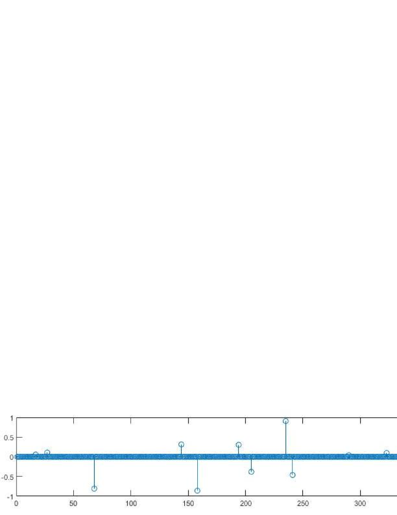
Fig.1 and Table.2 show the numerical results of our algorithm and other algorithms in two cases respectively. We give the graphs of original signal and recovered signal in Fig. 2.

Table 2: Numerical results for Example 1

Algorithms	Case 1		Case 2
Algorithms	Iter.	CPU(s)	Iter.	CPU(s)
Alg1	525	0.2447	809	1.2297
CHCAlg2	1347	0.5340	2595	3.0049
CHMAlg1	887	0.3496	1554	1.9651
HAMAlg1	971	0.3904	1577	1.5138
AKHAlg1	3427	1.3142	6723	6.4723

Refer to caption — (a) $K=20$ , $M=256$ , $N=512$

Remark 10

It can be seen from Fig.1 and Table 2 that the number of iterations and CPU time of our algorithm are better than other algorithms, indicating that our algorithm has better performance.

Example 2

We consider our algorithm to solve the variational inequality problem . The operator $A:{R^{m}}\to{R^{m}}$ is defined by $A(x):=Mx+q$ with $M=N{N^{T}}+S+D$ and $q\in{R^{m}}$ , where $N$ is an $m\times m$ matrix, $S$ is an $m\times m$ skew-symmetric matrix and $D$ is an $m\times m$ diagonal matrix. All entries of $N$ and $S$ are uniformly generated from $(-5,5)$ and all diagonal entries of $D$ are uniformly generated from $(0,0.3)$ . It is easy to see that $M$ is positive definite. Define the feasible set $C:={R_{m}}^{+}$ and use ${E_{n}}=\left\|{{x_{n}}}\right\|$ to measure the accuracy, and the stoping criterion is ${E_{n}}\leq 10^{-3}$ .

In the first experiment we consider the effect of relaxation coefficients $\theta_{n}$ on the performance of Algorithm 3.1. We choose $\mu=0.9$ , ${\alpha_{n}}=1$ , ${\beta_{n}}=0.1$ , ${\lambda_{1}}=0.1$ , ${\mu_{n}}=0$ and $p_{n}=\frac{1}{{{n^{2}}}}$ .

Table 3: The performances of Algorithm 3.1 for different values of

\theta_{n}

in Example 5.2

$\theta_{n}$	0.05	0.1	0.15	0.2	0.25	0.3	0.35	0.4	0.45
$Iter.$	16988	8521	5562	4035	3095	2454	1987	1360	1346
$CPU(s)$	1.8752	0.9888	0.6785	0.4804	0.3879	0.2910	0.2436	0.2246	0.1674

Table 3 shows that the performance comparison of Algorithm 3.1 for different values of $\theta_{n}$ . It can be seen that the performance of the algorithm becomes better with the increase of the relaxed parameter $\theta_{n}$ . This indicates that the increase of the relaxation coefficient value range is of great significance to improve the performance of the algorithm.

In second experiment we compared the performance of our algorithm with other algorithms. The following cases are considered

Case 1: $m=50$ ; Case 2: $m=100$ ; Case 3: $m=150$ ; Case 4: $m=200.$

The parameters for algorithms are chosen as

Alg1: $\mu=0.9$ , ${\alpha_{n}}=1-\frac{1}{{{{10}^{n}}}}$ , ${\beta_{n}}=0.1-\frac{1}{{1000+n}}$ , ${\theta_{n}}=0.45-\frac{1}{{1000+n}}$ , ${\mu_{n}}=0$ and ${p_{n}}=\frac{1}{{{n^{2}}}};$

HAMAlg1: $\mu=0.4$ , ${\lambda_{-1}}={\lambda_{0}}=0.3;$

CHCAlg2: $\mu=0.9$ , $\alpha=0.3$ , $\theta=0.4$ and ${\lambda_{1}}=1;$

YISAlg1: $\mu=0.9$ , ${\alpha_{n}}=0.2903$ , $\delta=0.0241$ , ${\theta_{n}}=1$ and ${\lambda_{1}}=0.1;$

AKHAlg1: $\mu=0.3$ , $\rho=0.1$ , $\varrho=0.9$ and ${\lambda_{0}}=1$ ;

CHMAlg1: $\mu=0.4$ , ${\alpha_{1}}=0.01$ , ${\alpha_{2}}=0.02$ and ${\lambda_{0}}=1$ .

Fig.3 and Table.4 show the performance comparison of our algorithm with other algorithms in four cases respectively.

Table 4: Numerical results for Example 2

Algorithms	$m=50$		$m=100$		$m=150$		$m=200$
Algorithms	Iter.	CPU(s)	Iter.	CPU(s)	Iter.	CPU(s)	Iter.	CPU(s)
Alg1	448	0.0191	642	0.0380	759	0.0968	1012	0.1681
CHCAlg2	723	0.0224	1048	0.0499	1234	0.1105	1644	0.2128
YISAlg1	600	0.0917	963	0.0635	1214	0.1374	1595	0.2125
HAMAlg1	779	0.0203	1142	0.0475	1355	0.1410	1751	0.1940
AKHAlg1	1049	0.0267	1425	0.0659	1691	0.1625	2371	0.2839
CHMAlg1	871	0.0331	1182	0.0637	1408	0.1366	1879	0.2158

Remark 11

It can be seen that our algorithm performs better than other algorithms for such problems as Example 5.2 from Fig.3 and Table 4.

Example 3

Let $H:={L_{2}}([1,2])$ with the norm

\left\|x\right\|:={(\int_{0}^{1}{x(t})^{2}}dt{)^{\frac{1}{2}}}.

and the inner product

\left\langle{x,y}\right\rangle:=\int_{0}^{1}{x(t)y(t)dt}.

Let $C:=\{x\in{L^{2}}([0,1]):\int_{0}^{1}{tx(t)dt=2}\}$ and define $A:{L^{2}}([0,1])\to{L^{2}}([0,1])$ by

Ax(t):=\max\{x(t),0\},x\in{L^{2}}([0,1]),t\in[0,1].

It is clear that $A$ is monotone and Lipschitz with $L=1$ . The orthogonal projection onto $C$ have the following explicit formula

{P_{C}}(x)(t):=x(t)-\frac{{\int_{0}^{1}{tx(t)dt-2}}}{{\int_{0}^{1}{{t^{2}}dt}}}t.

The example is taken from YI . Use ${E_{n}}=\left\|{{x_{n+1}}-{x_{n}}}\right\|$ to measure the accuracy. The stoping criterion is ${E_{n}}\leq 10^{-4}$ .

The following cases are considered

Case 1: ${x_{0}}=\frac{{97{t^{2}}+4t}}{{13}},{x_{1}}=\frac{{{t^{2}}-{e^{-7t}}}}{{250}};$

Case 2: ${x_{0}}=\frac{{97{t^{2}}+4t}}{{13}},{x_{1}}=\frac{{\sin(3t)+\cos(10t)}}{{100}};$

Case 3: ${x_{0}}=\frac{{{t^{2}}-{e^{-7t}}}}{{250}},{x_{1}}=\frac{{\sin(3t)+\cos(10t)}}{{100}};$

Case 4: ${x_{0}}=\frac{{\sin(3t)+\cos(10t)}}{{100}},{x_{1}}=\frac{{97{t^{2}}+4t}}{{13}}.$

The parameters for algorithms are chosen as

Alg1: $\mu=0.4$ , ${\alpha_{n}}=1-\frac{1}{{{{10}^{n}}}}$ , ${\beta_{n}}=0.1-\frac{1}{{1000+n}}$ , ${\theta_{n}}=0.45-\frac{1}{{1000+n}}$ and ${p_{n}}=\frac{1}{{{n^{2}}}};$

CHCAlg2: $\mu=0.4$ , $\alpha=0.3$ , $\theta=0.4$ and ${\lambda_{1}}=1;$

HAMAlg1: $\mu=0.4$ , ${\lambda_{-1}}={\lambda_{0}}=0.1;$

YISAlg1: $\mu=0.4$ , ${\alpha_{n}}=0.2250$ , $\delta=0.4950$ , ${\theta_{n}}=1$ and ${\lambda_{1}}=1.1;$

AKHAlg1: $\mu=0.4$ , $\rho=0.45$ , $\varrho=0.3$ and ${\lambda_{0}}=0.5;$

CHMAlg1: $\mu=0.4$ , ${\alpha_{1}}=0.01$ , ${\alpha_{2}}=0.02$ and ${\lambda_{0}}=1$ .

Table 5: Numerical results for Example 3

Algorithms	Case1		Case2		Case3		Case4
Algorithms	Iter.	CPU(s)	Iter.	CPU(s)	Iter.	CPU(s)	Iter.	CPU(s)
Alg1	32	0.0554	32	0.0499	18	0.0296	36	0.0416
CHCAlg2	40	0.0601	40	0.0616	24	0.0361	52	0.0664
VAMAlg1	47	0.0616	46	0.0558	22	0.0311	70	0.0974
YISAlg1	45	0.0894	45	0.0629	26	0.0457	53	0.0912
AKHAlg1	38	0.0746	39	0.0506	20	0.0277	46	0.0697
HAMAlg1	34	0.0651	37	0.0498	24	0.0343	70	0.0802

Remark 12

From Table 5 and Fig.4, we observe that our Algorithm 3.1 performs better and converges faster.

6 Conclusions

In this paper, we propose a new Tseng splitting method with double inertial extrapolation steps for solving monotone inclusion problems in real Hilbert spaces and establish the weak convergence, nonasymptotic $O(\frac{1}{\sqrt{n}})$ convergence rate, strong convergence and linear convergence rate of the proposed algorithm, respectively. Our method has the following advantages:

(i) Our method uses adaptive step sizes, which can be updated by a simple calculation without knowing the Lipschitz constant of the underlying operator.

(ii) Our method own double inertial extrapolation steps, in which inertial factor $\alpha_{n}$ can equal $1$ . This is not allowed in the corresponding algorithms of CV ; CH , where the only single inertial extrapolation step is considered and the inertial factor is bounded away from $1$ . From Table 1 in section 5, it can be seen Algorithm 3.1 with double inertial extrapolation steps outperforms the one with the single inertia.

(iii) Our method includes the corresponding methods considered in AB ; CV ; YI as special cases. Especially, when our algorithm is used to solve variational inequalities, the relaxed parameter sequence $\{\theta_{n}\}$ have larger choosing interval than the ones of YI . Via Table 3 in section 5, we observe that the performance of the algorithm becomes better with the increase of the relaxed parameter $\theta_{n}$ .

(iv) To the best of our knowledge, there are few available convergence rate results for algorithms with the double inertial extrapolation steps for solving variational inequalities and monotone inclusions. From numerical experiments in section 5, we can see that our algorithm has better efficiency than the corresponding algorithms in AB ; CV ; CH ; VA ; YI .

Acknowledgements.

This work was supported by the National Natural Science Foundation of China (11701479, 11701478), the Chinese Postdoctoral Science Foundation (2018M643434) and the Fundamental Research Funds for the Central Universities (2682021ZTPY040).

References

(1) Abubakar, J., Kumam, P., Hassan Ibrahim, A., Padcharoen, A.: Relaxed inertial Tsengs type method for solving the inclusion problem with application to image restoration. Mathematics. 8, 818 (2020)
(2) Alvarez, F., Attouch, H.: An inertial proximal method for maximal monotone operators via discretization of a nonlinear oscillator with damping. Set-Valued Analysis. 9, 3-11 (2001)
(3) Bauschke, H.H., Combettes, P.L.: Convex analysis and monotone operator theory in Hilbert spaces. Springer, New York (2011)
(4) Cai, G., Dong, Q.L., Peng, Y.: Strong convergence theorems for inertial Tseng’s extragradient method for solving variational inequality problems and fixed point problems. Optim. Lett. 15, 1457-1474 (2021)
(5) Cholamjiak, P., Hieu, D.V., Cho, Y.J.: Relaxed forward-backward splitting methods for solving variational inclusions and applications. J. Sci. Comput.88, 85 (2021)
(6) Cholamjiak, P., Hieu, D.V., Muu, L.D.: Inertial splitting methods without prior constants for solving variational inclusions of two operators. Bull. Iran. Math. Soc. (2022).https://doi.org/10.1007/s41980-022-00682-3
(7) Combettes, P.L., Wajs, V.: Signal recovery by proximal forward-backward splitting. SIAM Multiscale Model Simul. 4, 1168-1200 (2005)
(8) Çopur AK, Hacio $\breve{g}$ lu E, G $\ddot{u}$ rsoy F, et al.: An efficient inertial type iterative algorithm to approximate the solutions of quasi variational inequalities in real Hilbert spaces. J. Sci. Comput. 89:50(2022)
(9) Dong, Q., Jiang, D., Cholamjiak, P.: A strong convergence result involving an inertial forward-backward algorithm for monotone inclusions. J. Fixed Point Theory Appl. 19, 3097-3118 (2017)
(10) Duchi, J., Singer, Y.: Efficient online and batch learning using forward-backward splitting. J. Mach. Learn Res. 10, 2899-2934 (2009)
(11) Gibali, A., Thong, D.V.: Tseng type methods for solving inclusion problems and its applications. Calcolo 55, 55:49 (2018)
(12) Linh, N.X., Thong, D.V., Cholamjiak, P.: Strong convergence of an inertial extragradient method with an adaptive nondecreasing step size for solving variational inequalities. Acta Math. Sci. 42, 795-812 (2022)
(13) Lions, P.L., Mercier, B.: Splitting algorithms for the sum of two nonlinear operators. SIAM J. Numer. Anal. 16, 964-979 (1979)
(14) Liu, Q.: A convergence theorem of the sequence of Ishikawa iterates for quasi-contractive mappings. J. Math. Anal. Appl. 146, 301-305 (1990)
(15) Maing $\acute{e}$ , P. E.: Convergence theorems for inertial KM-type algorithms. J. Comput. Appl. Math. 219, 223-236 (2008)
(16) Opial, Z.: Weak convergence of the sequence of successive approximations for nonexpansive mappings. Bull. Am. Math. Soc. 73, 591-597 (1967)
(17) Padcharoen, A., Kitkuan, D., Kumam, W., Kumam, P.: Tseng methods with inertial for solving inclusion problems and application to image deblurring and image recovery problems. Comput. Math. Methods (2020). https://doi.org/10.1002/cmm4.1088
(18) Passty, G.B.: Ergodic convergence to a zero of the sum of monotone operators in Hilbert space. J. Math. Anal. Appl. 72, 383-390 (1979)
(19) Raguet, H., Fadili, J., Peyr $\acute{e}$ , G.: A generalized forward-backward splitting. SIAM J. Imaging Sci. 6, 1199-1226 (2013)
(20) Shehu, Y., Iyiola, O.S., Li, X.H., et al.: Convergence analysis of projection method for variational inequalities. Comput. Appl. Math. 38, 161 (2019)
(21) Shehu, Y., Iyiola, O.S., Reich, S.: A modified inertial subgradient extragradient method for solving variational inequalities. Optimization and Engineering, 23, 421-449.(2021)
(22) Tan, K.K., Xu, H.K.: Approximating fixed points of nonexpansive mappings by the Ishikawa iteration process. J. Math. Anal. Appl. 178, 301-308 (1993)
(23) Thong, D.V., Vinh, N.T. Cho, Y.J.: A strong convergence theorem for Tseng’s extragradient method for solving variational inequality problems. Optim. Lett. 14, 1157-1175 (2020)
(24) Thong, D.V., Yang, J., Cho, Y.J., Rassias, T.M.: Explicit extragradient-like method with adaptive stepsizes for pseudomonotone variational inequalities. Optim. Lett. 15, 2181-2199 (2021)
(25) Tseng, P.: A modified forward-backward splitting method for maximal monotone mapping. SIAM J. Control Optim. 38, 431-446 (2000)
(26) Van Hieu, D., Anh, P.K. Muu, L.D.: Modified forward-backward splitting method for variational inclusions. 4OR-Q J. Oper. Res. 19, 127-151 (2021)
(27) Wang, Z.B., Chen, X., Jiang, Y,, et al.: Inertial projection and contraction algorithms with larger step sizes for solving quasimonotone variational inequalities. J. Glob. Optim. 82:499-522 (2022)
(28) Xu, H.K.: Iterative algorithms for nonlinear operators. J. Lond. Math. Soc. 66, 240-256 (2002)
(29) Yao, Y., Iyiola, O.S. Shehu, Y.: Subgradient extragradient method with double inertial steps for variational inequalities. J. Sci. Comput. 90, 71 (2022)