Truncated string state space approach and its application to nonintegrable spin- Heisenberg chain
Abstract
By circumventing the difficulty of obtaining exact string state solutions to Bethe ansatz equations, we devise a truncated string state space approach for investigating spin dynamics in a nonintegrable spin- Heisenberg chain subjected to a staggered field at various magnetizations. The obtained dynamical spectra reveal a series of elastic peaks at integer multiples of the ordering wave vector , indicating the presence of multi- Bethe string states within the ground state. The spectrum exhibits a separation between different string continua as the strength of the staggered field increases at low magnetization, reflecting the confinement of the Bethe strings. This approach provides a unified string-state-based framework for understanding spin dynamics in low-dimensional nonintegrable Heisenberg models, which has a successful application to observations across various phases of the quasi-one-dimensional antiferromagnet .
I Introduction
One-dimensional quantum systems characterized by exact solutions and quantum integrability offer a fascinating arena to study many-body physics. Notable examples include the one-dimensional (1D) spin- XXZ model [1, 2, 3, 4], Gaudin-Yang model [5, 6, 7], Lieb-Liniger model [8, 9], and quantum Ising models [10, 11, 12, 13]. Although these models have paved the way for determining the eigenstates and eigenenergies of those systems, it has long been a challenge to calculate their form factors and thus dynamical response, which was partly tackled recently [14, 7, 15, 16, 17, 18, 19, 20]. Empowered by the theoretical development, the spin dynamics of celebrated many-body quasiparticles, such as spinons [21, 22, 23], strings [24, 25, 26], [27, 28, 29, 30, 31] and particles [32, 33, 34], have been extensively explored, providing crucial guidance for the experimental observations in quasi-1D materials [3, 35, 36, 37, 38, 39, 40, 30, 31]. This progress has led to the cooperative effort of both theorists and experimentalists to unveil the intricate nature of these exotic phenomena.
Bearing real materials in mind, it becomes crucial to ask how robust integrable physics is against nonintegrable perturbations that may partially or fully break the conservation laws of integrable systems. This has inspired extensive research focused on nonintegrable models such as spin- ladders [41, 42], chains with a staggered magnetic field [43, 44], frustrated spin chains [45], and dimerized spin chains [46, 47]. Most studies are performed by using effective field theory [43, 44] or numerical methods such as the exact diagonalization (ED) [45, 46], matrix product state [47], and quantum Monte Carlo methods [48]. However, on the one hand, numerical methods in general lack a clear understanding of the essential physical picture, on the other hand, the effective field theory can provide only limited insight within the low-energy and long-wavelength limit. Therefore, a method able to go beyond those limitations is always desired.
At first glance it may seem promising to apply Bethe states to study nonintegrable systems. However, a notorious open problem persists: finding the precise complex solutions of the Bethe ansatz equation (BAE) for string states [24, 49, 50, 51, 52, 53]. In the past few decades, many approaches have been explored, including a carefully-designed iterative method [54] and a rational -system method [55, 56, 57]. The former can easily access large system size but suffers from many unphysical solutions with repeated roots. Although the latter can solve the BAE for all exact solutions simultaneously, it is limited to a small system size. Those shortcomings impede the practical application of Bethe states to understand nonintegrable systems of reasonable size.
In this paper, we first outline a solving machine for the spin- Heisenberg chain, which can obtain exact solutions for Bethe string states. Based on these string states, we develop a truncated string-state-space approach (TS3A) to study nonintegrable Hamiltonian, specifically the spin- Heisenberg chain with a staggered field. The TS3A can determine the eigenstate and eigenenergy for the nonintegrable Hamiltonian in the truncated Hilbert space. Additionally, we evaluate its efficiency for small systems under various truncation schemes, involving different energy cutoffs and string lengths, by comparing its performance to that of ED calculations.
Following the TS3A, we analyze the nonintegrable spin dynamics in the spin- Heisenberg chain with staggered field characterized by wavevector . In addition to the -ordering of the system, a series of elastic peaks appear at , indicating the ground state contains multi- Bethe string states. Moreover, the staggered field plays the role of the confining field for the Bethe string states, constraining the motion of spins along the chain. The confinement of Bethe strings results in two separated continua in dynamical spectra at low magnetization. Notably, the above results were successfully applied to experimental observations of the quasi-1D antiferromagnet , aligning with the unified Bethe-string-based framework provided by the TS3A [58].
The rest of this paper is organized as follows. Section II introduces the Hamiltonian of the 1D Heisenberg model with a staggered field. Section III illustrates the Bethe string state and then presents a method for obtaining exact solutions from the BAE. The framework of the TS3A is developed, and its efficiency is investigated in Sec. IV. Then Sec. V discusses the spin dynamics of the nonintegrable Hamiltonian. Section VI contains the conclusion and outlook.
II Model
Our parent Hamiltonian is the 1D Heisenberg spin- model with longitudinal field ,
| (1) |
with being the total number of sites, being antiferromagnetic coupling, and being spin operators with components () at site . With the introduction of a staggered field which couples to the spin chain, the total Hamiltonian becomes nonintegrable,
| (2) |
where
| (3) |
is the strength of the staggered field, and the ordering wave vector , where the magnetization density , which is the ratio of magnetization to its saturation value . In practice, the staggered field can be effectively induced from three-dimensional (3D) magnetic ordering of quasi-1D materials, such as [59, 60, 61, 58], [62] and [30]. We note that the staggered field can be both commensurate and incommensurate, depending on whether is a rational or irrational number, respectively.

III Exact Bethe string state
In this section, we begin with an introduction to the coordinate Bethe ansatz and Bethe string states for the Hamiltonian [Eq. (1)]. Then an efficient method is presented for obtaining the exact solutions from the BAE.
III.1 Bethe ansatz and the Bethe string state
Due to U(1) symmetry of [Eq. (1)] the magnetization is the conserved quantity, where is the number of down spins, i.e. magnons, with respect to the fully polarized state with all up spins . In the coordinate Bethe ansatz [63, 64, 65], the eigenstate of [Eq. (1)] is the Bethe state with magnons, which is determined by a set of rapidities satisfying the BAE,
| (4) |
with . The corresponding quasi-momentum . These rapidities manifest as either complex-conjugate pairs or real numbers [Fig. 1(a)] [66]. The pair of complex rapidities implies significant physical property: the corresponding magnons exhibit an intriguing phenomenon in coordinate space, forming effectively bounded magnons commonly known as “Bethe string” [24, 64, 67]. And the length of the string is determined by the number of rapidities with a common real center. Intuitively, Bethe string () of length is a “big” quasiparticle in which bounded magnons move coherently, referred to as a -string [Fig. 1(b)-(d)]. When , the 1-string is just the unbound magnon. Correspondingly, the rapidities of a string takes the form [24, 49]
| (5) |
where denotes the th magnon in the -string. The number of -strings is denoted as , and label different -strings with the same length . Thus we have for an -magnon Bethe state. We refer to as the string center which gives the real part of the -string if the deviation is omitted. Under the assumption , we obtain eigenenergy of a Bethe string state, , with . Therefore, we can show the relation between energy and quasi-momentum for different strings in Fig. 1(e). For finite , the eigenenergy becomes with .
To ensure clarity in terminology, we refer to a Bethe state with all magnons being as the 1-string state. For , we classify an -string state with and . When , it is simply referred to as the -string state. This convention can be consistently extended to cover other cases.
| unphysical | 0.4458 | 0.4458 | 0.1803 | ||
| physical | 0.1807 |
III.2 Exact solution
To characterize Bethe string states, the initial step is to obtain rapidities () by solving the BAE [Eq. (4)]. This is commonly achieved by considering the logarithmic form of BAE,
| (6) |
where , and is the corresponding Bethe quantum number. Equation (6) is highly efficient for finding the real solutions using the iterative method [54, 68]. However, for complex solutions, we first need to consider the reduced Bethe equation with [67],
| (7) |
with , and , with , and . The is referred to as the reduced Bethe quantum number. The Eq. (7) can also be tackled iteratively to obtain the string centers , whose associated complex solutions are constructed from Eq. (5) with . Nevertheless, these solutions are generally not exact because they disregard the finite deviation . By utilizing the solutions obtained with Eq. (7) as an initial guess, the finite deviation is accessible for a majority of the string states following the method in Ref. [54]. A summary is presented in Appendix. A.
However, the strategy introduced above fails to generate all exact solutions when the number of lattice sites exceeds , with example in Table 1 and details in Appendix A. The limitations arise from the generation of repeated real rapidities in string states which are physically forbidden [69, 70]. The key to solving the problem is that the repeated real rapidities actually form a complex conjugate pair with a minor imaginary part (typically ). To implement the observation into the algorithm, we divide and conquer, with details in Appendix A.3. For instance, for a 3-string state, the typical rapidity pattern is that three of them share a common real part up to a finite deviation , while the remaining rapidities are all real. However, when we encounter repeated real rapidities (in first row of Table 1), usually involving the 3-string center and one real rapidity, we introduce a small imaginary part to create a complex conjugate pair. This pair and other rapidities are then treated as a new initial guess for the BAE, from which we are able to efficiently obtain the exact solution, the second row in Table 1.
Before ending this section, it is imperative to underscore the importance of exact solutions. As shown in the Appendix B, the determinant expression of becomes divergent when represents string states with zero deviation due to the failure of regularization. Therefore, assuming may not be appropriate for our subsequent TS3A approach. Therefore, the practical route is to consider the string states with finite .


IV Truncated string-state-space approach
In many physical problems, our focus is on the low-energy subspace rather than the entire Hilbert space [71, 72, 73]. In this study, we employ the TS3A method, as illustrated in [Fig. 1f], to gain insights into the low-energy physics of nonintegrable Heisenberg models Eq. (2). The detailed construction is as follows.
When considering a nonintegrable perturbation, such as [Eq. (3)], the Bethe string state is no longer the eigenstate. Therefore, it becomes necessary to find out the new ground state and low-energy excited states before conducting any calculations of physical quantities, such as correlation functions. The first step is to construct the matrix representation of the nonintegrable Hamiltonian [Eq. (2)] within a truncated low-energy subspace of Bethe string states, denoted as , with . The truncated dimension of is typically much less than , which is determined by the energy cutoff and types of Bethe string states . Following the diagonalization of , a new ground state and low-energy excited states are obtained, which are considered as approximate eigenstates of the Hamiltonian .
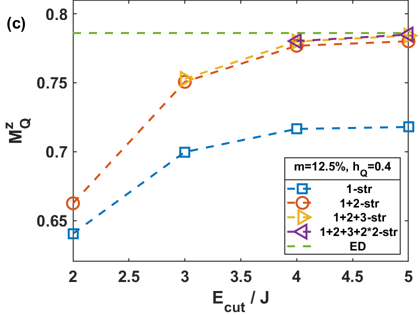
However, an immediate question arises: How do we select the types of Bethe string states and determine the energy cutoff? To answer the first question, we investigate the form factor between Bethe string states. It is evident from Fig. 2(a) that the form factors for string states generally diminish rapidly as the difference in string length increases. For instance, the ground state of Eq. (1) is a 1-string state, and then we can safely truncate the string state space into relevant subspace in terms of string lengths. For the second issue, we study the asymptotic behavior of ground state energy and the staggered magnetization as the energy cutoff of the truncated space increase. In Fig. 2(b,c), the calculation includes all allowed string states within a given . As increases the results converge rapidly and approach the exact values obtained from the ED calculation. Notably, even if only 1- and 2-string states are considered, the obtained results are already very close to the exact values, while the impact of 3- and -string states is marginal. This phenomenon confirms the suggestion that the relevant string states primarily arise from those with small length differences, as illustrated in Fig. 2(a).
V Spin dynamics
To investigate nonintegrable spin dynamics of [Eq. (2)], we focus on the zero-temperature dynamical structure factor (DSF) for spin along longitudinal () direction (),
| (8) |
with being the transfer momentum and being the transfer energy between the ground state and excited states , whose energies are and , respectively. In the following calculation, the eigenstates and are obtain by the TS3A developed in Sec. IV. The form factor is deeply related to the form factor of Bethe string states, which can be elegantly expressed in terms of determinant [25, 74, 75, 22, 23, 26], with a summary in Appendix B.


To begin with, we investigate the TS3A results under different truncation schemes for , , and . In Fig. 3(a1-a4), the DSF is calculated with different selected string types and fixed energy cutoff , showing that 1- and 2-strings are the dominant states in the spin dynamics. In Fig. 3(b1-b4), the DSF is calculated with different energy cutoff and fixed string types (including 1-, 2-, 3- and -string), showing that the dynamical spectrum converges quickly as increases. Furthermore, we compare the DSF results at obtained from TS3A to that of the ED method [76, 77], whose results reveal a remarkable agreement in Fig. 4. This excellent comparison suggests that the TS3A is a highly efficient method for studying the nonintegrable spin dynamics.
In the following, we present the DSF results obtained from the TS3A at . Due to the staggered field perturbation term [Eq. (3)], where , the non-vanishing matrix element of only appears between Bethe states with momentum difference . As a result, the ground state consists of Bethe states with momenta . For static structure factor , a series of staggered-field-induced peaks appear at (), manifesting the presence of multi- Bethe states in the ground state. For instance, in Fig. 5(a-d), there are satellite peaks at in addition to the predominant peaks at , with .


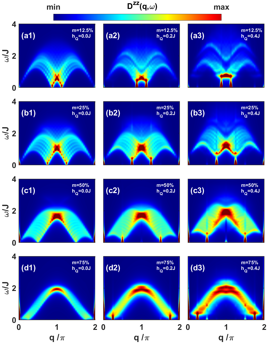
In Fig. 6, when , the dynamical spectra exhibit gapless excitations at , and the 2-string states are barely separated from the broad continuum of 1-string states. When , an energy gap emerges both near the elastic line and between the continua of 1- and 2-string states. This phenomenon arises because the staggered field acts as a confining field for the Heisenberg spin chains, effectively restricting the motion of spins [78, 79, 80, 43, 44]. These induced gaps reflect the energy cost for the excitation of Bethe strings, which is known as the confinement of Bethe strings. At small magnetization [Fig. 6(a1-a3)], 2-string states are effectively confined and become separated from the 1-string continuum. However, as magnetization increases, the 2-string continuum gradually dissipates into higher energy ranges.
Notably, the capability for larger size calculation of TS3A not only reduces the finite size effect but also renders the characteristics of spectra more transparent and discernible. And, the TS3A offers two key advantages compared to the ED method: First, it has higher efficiency, facilitating much larger systems (); second, it naturally provides a unified Bethe-string-based physical picture for understanding the underlying physics.
We conclude this section by emphasizing that our model and findings offer a direct application in comprehending the low-energy spin dynamics observed in the quasi-1D antiferromagnet [59, 61, 58]. In this material, the low-energy effective Hamiltonian is described by the 1D Heisenberg models Eq. (1), and Eq. (2) if the material is 3D ordered. In Fig. 5(e), the quasi-elastic signals obtained from neutron scattering align with the theoretical predictions, providing compelling evidence for the coexistence of multi- Bethe states in the ordered phase of . Moreover, the staggered field, arising from the 3D ordering, plays the role of a confining field coupled with the spin chains within the material. As a result, the distinctive features characterizing the confined string states are observed through the inelastic neutron scattering spectra of [58].
VI Conclusion
We exploited an efficient routine to find exact solutions for the Bethe string states from the BAE of the spin- Heisenberg spin chain. Based on the exact solutions we further developed the TS3A which enabled us to determine eigenstates and eigenenergies of nonintegrable spin- Heisenberg systems with U(1) symmetry preserved. The method was then applied to systematically study the spin dynamics of the spin- Heisenberg spin chain under staggered field. In the dynamical spectra, we revealed a series of elastic peaks located at the integer multiples of the ordering wavevector , signifying the existence of multi- Bethe string states within the ground state. Moreover, the staggered field serves as a confining field for Bethe string states, inducing confinement gaps between the continua of 1- and 2-string states.
Our TS3A machine offers a Bethe-string-based scenario, contributing to a more comprehensive understanding of Heisenberg spin systems. We have demonstrated the efficiency and validity of this framework by interpreting experimental observations of the quasi-1D antiferromagnet . This intriguing consistency between theoretical predictions based on the TS3A and experimental results motivates its extended application to ladder and two-dimensional Heisenberg systems. This broadening of scope not only enhances the versatility of the Bethe string picture but also transcends its conventional one-dimensional limitations.
Acknowledgments
We thank Yunfeng Jiang for helpful discussion. This work is supported by National Natural Science Foundation of China No. 12274288 and the Innovation Program for Quantum Science and Technology Grant No. 2021ZD0301900, and the Natural Science Foundation of Shanghai with grant No. 20ZR1428400.
Appendix A Iterative method for exact solution
This appendix present the iterative method for solving the Bethe equation. Note that it’s sufficient to solve the highest weight state containing only finite rapidities, while other states can be obtained by adding infinite rapidities [54].
A.1 Deviation
For the 1-string state, all rapidities are real, which can be directly solved from the iterative form of the Bethe equation,
| (9) |
where is the corresponding Bethe quantum number for .
For the string state, there is at least one complex rapidity in the pattern of Eq. (5). To obtain the corresponding rapidities, we convert the reduced Bethe equation Eq. (7) into the iterative form,
| (10) |
where is the corresponding reduced Bethe quantum number for string centers . Following Eq. (5), the complex string states is constructed from with .
A.2 Deviation
To determine the exact deviation , the strategy becomes more intricate for the XXX model [54] and for the gapped XXZ model [26]. Here, we only consider 2- and 3-string states for illustration.
For a string with length , its two complex rapidities are , where the deviations are purely imaginary, and . Then we can have the first-order deviation,
| (11) |
Next, utilizing the first-order deviation, we can determine the true Bethe quantum number from reduced one ,
| (12) |
where
| (13) |
Then, considering the sum of the logarithmic Bethe equations Eq. (6),
| (14) |
and the deformation of Bethe equation Eq. (4),
| (15) |
we can solve for , along with from the Bethe equations Eq. (6) of 1-strings.
For a string with length , it contains three rapidities, , , where . Then we can have the first-order deviation,
| (16) |
We note that for the 3-string, must hold, which leads to the fact that must be a wide pair with . Then, we still need two more equations to solve the true Bethe quantum numbers , . The first equation is the sum of the logarithmic Bethe equations Eq. (6),
| (17) |
Another necessary equation is the sum of logarithmic BAEs of
| (18) |
Let A be the right hand side of Eq. (18). Because , is the even(odd) integer number in when is even(odd). Therefore,
| (19) |
Now combing the wide pair condition (), Eqs. (17), and (19), and can be determined. The Bethe quantum number for real rapidities can be shown to be of the following expression,
| (20) |
To solve rapidities, we first need the sum of logarithmic BAE of and without setting and to be zero
| (21) |
The second equation is the sum of logarithmic BAE of Eq. (18). The third one is obtained from Bethe equation Eq. (4) after some simple manipulation
| (22) |
The logarithmic Bethe equations Eq. (6) are also needed for real rapidities.
| 1. unphysical | 4 | 0.495521913637784 + 0.962224932131036i | -3.632275481625215 | |
| 3 | 0.445792844757107 + 0.000000000000000i | |||
| 5 | 0.495521913637784 - 0.962224932131036i | |||
| 2 | 0.180317318693691 + 0.000000000000000i | |||
| 3 | 0.445792844757134 + 0.000000000000000i | |||
| 2. physical | 4 | 0.491814213695900 + 0.961471132379077i | -3.60069325626932 | |
| 3 | 0.444763506448628 + 0.018770199402376i | |||
| 5 | 0.491814213695898 - 0.961471132379085i | |||
| 2 | 0.180714318631831 + 0.000000000000000i | |||
| 3 | 0.444763506448649 - 0.018770199402378i |
Here, we present the 3-string state results of and obtained from the above iterative method in the first set of Table 2. We can observe that two real rapidities coincide, one is the string center and another is a 1-string. However, it is unphysical because of the incorrect eigenenergy and the absence of wave function under this set of solutions.
A.3 Repeated real rapidities
To tackle the issue of the repeated real rapidities of , we introduce a small imaginary part to create a complex conjugate pair, as required by the BAE. Now, we have two complex conjugate pairs. The first pair has a small imaginary part, , while the second one has a larger imaginary part around , . Note that 4 complex rapidities need 4 equations to solve. The strategy is similar to the procedures mentioned above. Two equations come from the sum of logarithmic Bethe equations of and . Another two equations come from the original Bethe equations of and . Combining the logarithmic Bethe equations for real rapidity, we could solve , , and real rapidities .
Appendix B The determinant formula
B.1 Norm of the Bethe state
B.2 Form factors
The non-zero form factors associated with correspond to states characterized by equal magnon numbers,
| (25) |
where , and is the eigen-momentum of Bethe state . The matrix elements of and matrix are defined as
| (26) |
| (27) |
respectively. Here we note that both the 2- and 3-string states with can cause divergence in the matrix Eq. (27). However, the divergence can not be regularized since there are no common terms in matrix Eq. (26).
References
- Jimbo and Miwa [1995] M. Jimbo and T. Miwa, Algebraic Analysis of Solvable Lattice Models (American Mathematical Society, 1995).
- Franchini [2017] F. Franchini, An Introduction to Integrable Techniques for One-Dimensional Quantum Systems, Vol. 940 (Springer, Cham, 2017).
- Yang et al. [2023a] J. Yang, X. Wang, and J. Wu, Magnetic excitations in the one-dimensional Heisenberg-Ising model with external fields and their experimental realizations, J. Phys. A: Math. Theor. 56, 013001 (2023a).
- He et al. [2017] F. He, Y. Jiang, Y.-C. Yu, H.-Q. Lin, and X.-W. Guan, Quantum criticality of spinons, Phys. Rev. B 96, 220401 (2017).
- Gaudin [1967] M. Gaudin, Un systeme a une dimension de fermions en interaction, Phys. Lett. A 24, 55 (1967).
- Yang [1967] C. N. Yang, Some exact results for the many-body problem in one dimension with repulsive delta-function interaction, Phys. Rev. Lett. 19, 1312 (1967).
- Guan et al. [2013] X.-W. Guan, M. T. Batchelor, and C. Lee, Fermi gases in one dimension: From bethe ansatz to experiments, Rev. Mod. Phys. 85, 1633 (2013).
- Lieb and Liniger [1963] E. H. Lieb and W. Liniger, Exact Analysis of an Interacting Bose Gas. i. The General Solution and the Ground State, Phys. Rev. 130, 1605 (1963).
- Lieb [1963] E. H. Lieb, Exact Analysis of an Interacting Bose Gas. II. The Excitation Spectrum, Phys. Rev. 130, 1616 (1963).
- Pfeuty [1970] P. Pfeuty, The one-dimensional Ising model with a transverse field, Ann. Phys. 57, 79 (1970).
- Niemeijer [1967] T. Niemeijer, Some exact calculations on a chain of spins 1/2, Physica 36, 377 (1967).
- Boyanovsky [1989] D. Boyanovsky, Field theory of the two-dimensional Ising model: Conformal invariance, order and disorder, and bosonization, Phys. Rev. B 39, 6744 (1989).
- A. B. Zamolodchikov [1989] A. B. Zamolodchikov, Integrables of motion and S-matrix of the (scaled) T = Ising model with magnetic field, Int. J. Mod. Phys. A 4, 4235 (1989).
- Li et al. [2023] R.-T. Li, S. Cheng, Y.-Y. Chen, and X.-W. Guan, Exact results of dynamical structure factor of Lieb-Liniger model, J. Phys. A: Math. Theor. 56, 335204 (2023).
- Guan and Andrei [2018] H. Guan and N. Andrei, Quench Dynamics of the Gaudin-Yang Model, arXiv.1803.04846 (2018).
- Kitanine et al. [1999] N. Kitanine, J. M. Maillet, and V. Terras, Form factors of the XXZ Heisenberg spin-1/2 finite chain, Nucl. Phys. B 554, 647 (1999).
- Kitanine et al. [2000] N. Kitanine, J. M. Maillet, and V. Terras, Correlation functions of the XXZ Heisenberg spin-1/2 chain in a magnetic field, Nucl. Phys. B 567, 554 (2000).
- Yang et al. [2022] J. Yang, W. Yuan, T. Imai, Q. Si, J. Wu, and M. Kormos, Local dynamics and thermal activation in the transverse-field ising chain, Phys. Rev. B 106, 125149 (2022).
- Iorgov et al. [2011] N. Iorgov, V. Shadura, and Y. Tykhyy, Spin operator matrix elements in the quantum Ising chain: fermion approach, J. Stat. Mech. 2011, P02028 (2011).
- Mussardo [2020] G. Mussardo, Statistical Field Theory: An Introduction to Exactly Solved Models in Statistical Physics (Oxford University Press, 2020).
- Caux and Hagemans [2006a] J.-S. Caux and R. Hagemans, The four-spinon dynamical structure factor of the heisenberg chain, Journal of Statistical Mechanics: Theory and Experiment 2006, P12013 (2006a).
- Caux et al. [2008a] J.-S. Caux, J. Mossel, and I. P. Castillo, The two-spinon transverse structure factor of the gapped heisenberg antiferromagnetic chain, Journal of Statistical Mechanics: Theory and Experiment 2008, P08006 (2008a).
- Castillo [2020] I. P. Castillo, The exact two-spinon longitudinal dynamical structure factor of the anisotropic XXZ model, arXiv:2005.10729 [cond-mat] (2020).
- Takahashi [1971] M. Takahashi, One-Dimensional Heisenberg Model at Finite Temperature, Prog. Theor. Phys. 46, 401 (1971).
- Kohno [2009] M. Kohno, Dynamically Dominant Excitations of String Solutions in the Spin-1/2 Antiferromagnetic Heisenberg Chain in a Magnetic Field, Phys. Rev. Lett. 102, 037203 (2009).
- Yang et al. [2019] W. Yang, J. Wu, S. Xu, Z. Wang, and C. Wu, One-dimensional quantum spin dynamics of Bethe string states, Phys. Rev. B 100, 184406 (2019).
- Coldea et al. [2010] R. Coldea, D. A. Tennant, E. M. Wheeler, E. Wawrzynska, D. Prabhakaran, M. Telling, K. Habicht, P. Smeibidl, and K. Kiefer, Quantum criticality in an Ising chain: Experimental evidence for emergent symmetry, Science 327, 177 (2010).
- Wu et al. [2014] J. Wu, M. Kormos, and Q. Si, Finite-temperature spin dynamics in a perturbed quantum critical ising chain with an symmetry, Phys. Rev. Lett. 113, 247201 (2014).
- Wang et al. [2021] X. Wang, H. Zou, K. Hódsági, M. Kormos, G. Takács, and J. Wu, Cascade of singularities in the spin dynamics of a perturbed quantum critical ising chain, Phys. Rev. B 103, 235117 (2021).
- Zou et al. [2021] H. Zou, Y. Cui, X. Wang, Z. Zhang, J. Yang, G. Xu, A. Okutani, M. Hagiwara, M. Matsuda, G. Wang, G. Mussardo, K. Hódsági, M. Kormos, Z. He, S. Kimura, R. Yu, W. Yu, J. Ma, and J. Wu, spectra of quasi-one-dimensional antiferromagnet under transverse field, Phys. Rev. Lett. 127, 077201 (2021).
- Wang et al. [2023] X. Wang, K. Puzniak, K. Schmalzl, C. Balz, M. Matsuda, A. Okutani, M. Hagiwara, J. Ma, J. Wu, and B. Lake, Spin dynamics of the particles (2023), arXiv:2308.00249 [cond-mat.str-el] .
- Gao et al. [2024] Y. Gao, X. Wang, N. Xi, Y. Jiang, R. Yu, and J. Wu, Spin dynamics and dark particle in a weak-coupled quantum ising ladder with spectrum (2024), arXiv:2402.11229 [cond-mat.str-el] .
- Xi et al. [2024] N. Xi, X. Wang, Y. Gao, Y. Jiang, R. Yu, and J. Wu, Emergent spectrum and topological soliton excitation in CoNb2O6 (2024), arXiv:2403.10785 [cond-mat.str-el] .
- LeClair et al. [1998] A. LeClair, A. Ludwig, and G. Mussardo, Integrability of coupled conformal field theories, Nucl. Phys. B 512, 523 (1998).
- Lake et al. [2013] B. Lake, D. A. Tennant, J.-S. Caux, T. Barthel, U. Schollwöck, S. E. Nagler, and C. D. Frost, Multispinon Continua at Zero and Finite Temperature in a Near-Ideal Heisenberg Chain, Phys. Rev. Lett. 111, 137205 (2013).
- Wang et al. [2018] Z. Wang, J. Wu, W. Yang, A. K. Bera, D. Kamenskyi, A. T. M. N. Islam, S. Xu, J. M. Law, B. Lake, C. Wu, and A. Loidl, Experimental observation of Bethe strings, Nature 554, 219 (2018).
- Bera et al. [2020] A. K. Bera, J. Wu, W. Yang, R. Bewley, M. Boehm, J. Xu, M. Bartkowiak, O. Prokhnenko, B. Klemke, A. T. M. N. Islam, J. M. Law, Z. Wang, and B. Lake, Dispersions of many-body Bethe strings, Nat. Phys. 16, 625 (2020).
- Wang et al. [2019] Z. Wang, M. Schmidt, A. Loidl, J. Wu, H. Zou, W. Yang, C. Dong, Y. Kohama, K. Kindo, D. I. Gorbunov, S. Niesen, O. Breunig, J. Engelmayer, and T. Lorenz, Quantum Critical Dynamics of a XXZ in a Longitudinal Field: Strings vs Fractional Excitations, Phys. Rev. Lett. 123, 067202 (2019).
- Zhang et al. [2020] Z. Zhang, K. Amelin, X. Wang, H. Zou, J. Yang, U. Nagel, T. Rõõm, T. Dey, A. A. Nugroho, T. Lorenz, J. Wu, and Z. Wang, Observation of particles in an Ising chain antiferromagnet, Phys. Rev. B 101, 220411 (2020).
- Amelin et al. [2020] K. Amelin, J. Engelmayer, J. Viirok, U. Nagel, T. Rõõm, T. Lorenz, and Z. Wang, Experimental observation of quantum many-body excitations of symmetry in the Ising chain ferromagnet , Phys. Rev. B 102, 104431 (2020).
- Steinigeweg et al. [2016] R. Steinigeweg, J. Herbrych, X. Zotos, and W. Brenig, Heat Conductivity of the Heisenberg Spin-1/2 Ladder: From Weak to Strong Breaking of Integrability, Phys. Rev. Lett. 116, 017202 (2016).
- Batchelor et al. [2007] M. T. Batchelor, X. W. Guan, N. Oelkers, and Z. Tsuboi, Integrable models and quantum spin ladders: comparison between theory and experiment for the strong coupling ladder compounds, Adv. Phys. 56, 465 (2007).
- Essler et al. [1997] F. H. L. Essler, A. M. Tsvelik, and G. Delfino, Quasi-one-dimensional spin-1/2 Heisenberg magnets in their ordered phase: Correlation functions, Phys. Rev. B 56, 11001 (1997).
- Starykh and Balents [2014] O. A. Starykh and L. Balents, Excitations and quasi-one-dimensionality in field-induced nematic and spin density wave states, Phys. Rev. B 89, 104407 (2014).
- Bonča et al. [1994] J. Bonča, J. P. Rodriguez, J. Ferrer, and K. S. Bedell, Direct calculation of spin stiffness for spin-1/2 Heisenberg models, Phys. Rev. B 50, 3415 (1994).
- Heidrich-Meisner et al. [2003] F. Heidrich-Meisner, A. Honecker, D. C. Cabra, and W. Brenig, Zero-frequency transport properties of one-dimensional spin-1/2 systems, Phys. Rev. B 68, 134436 (2003).
- Keselman et al. [2020] A. Keselman, L. Balents, and O. A. Starykh, Dynamical Signatures of Quasiparticle Interactions in Quantum Spin Chains, Phys. Rev. Lett. 125, 187201 (2020).
- Zhou et al. [2021] C. Zhou, Z. Yan, H.-Q. Wu, K. Sun, O. A. Starykh, and Z. Y. Meng, Amplitude Mode in Quantum Magnets via Dimensional Crossover, Phys. Rev. Lett. 126, 227201 (2021).
- Takahashi and Suzuki [1972] M. Takahashi and M. Suzuki, One-Dimensional Anisotropic Heisenberg Model at Finite Temperatures, Prog. Theor. Phys. 48, 2187 (1972).
- Fujita et al. [2003] T. Fujita, T. Kobayashi, and H. Takahashi, Large-N behaviour of string solutions in the Heisenberg model, J. Phys. A: Math. Gen. 36, 1553 (2003).
- Ilakovac et al. [1999] A. Ilakovac, M. Kolanović, S. Pallua, and P. Prester, Violation of the string hypothesis and the Heisenberg XXZ spin chain, Phys. Rev. B 60, 7271 (1999).
- Isler and Paranjape [1993] K. Isler and M. B. Paranjape, Violations of the string hypothesis in the solutions of the Bethe ansatz equations in the XXX-Heisenberg model, Phys. Lett. B 319, 209 (1993).
- Essler et al. [1992] F. H. L. Essler, V. E. Korepin, and K. Schoutens, Fine structure of the Bethe ansatz for the spin-1/2 Heisenberg XXX model, J. Phys. A: Math. Gen. 25, 4115 (1992).
- Hagemans and Caux [2007] R. Hagemans and J.-S. Caux, Deformed strings in the Heisenberg model, J. Phys. A: Math. Theor. 40, 14605 (2007).
- Marboe and Volin [2017] C. Marboe and D. Volin, Fast analytic solver of rational Bethe equations, J. Phys. A: Math. Theor. 50, 204002 (2017).
- Bajnok et al. [2020] Z. Bajnok, E. Granet, J. L. Jacobsen, and R. I. Nepomechie, On generalized Q-systems, J. High Energ. Phys. 2020 (3), 177.
- Hou et al. [2024] J. Hou, Y. Jiang, and R.-D. Zhu, Spin- rational -system, SciPost Phys. 16, 113 (2024).
- Yang et al. [2023b] J. Yang, T. Xie, S. E. Nikitin, J. Wu, and A. Podlesnyak, Confinement of many-body bethe strings, Phys. Rev. B 108, L020402 (2023b).
- Wu et al. [2019] L. S. Wu, S. E. Nikitin, Z. Wang, W. Zhu, C. D. Batista, A. M. Tsvelik, A. M. Samarakoon, D. A. Tennant, M. Brando, L. Vasylechko, M. Frontzek, A. T. Savici, G. Sala, G. Ehlers, A. D. Christianson, M. D. Lumsden, and A. Podlesnyak, Tomonaga-Luttinger liquid behavior and spinon confinement in , Nat. Commun. 10, 698 (2019).
- Fan et al. [2020] Y. Fan, J. Yang, W. Yu, J. Wu, and R. Yu, Phase diagram and quantum criticality of Heisenberg spin chains with Ising anisotropic interchain couplings, Phys. Rev. Res. 2, 013345 (2020).
- Nikitin et al. [2021] S. E. Nikitin, S. Nishimoto, Y. Fan, J. Wu, L. S. Wu, A. S. Sukhanov, M. Brando, N. S. Pavlovskii, J. Xu, L. Vasylechko, R. Yu, and A. Podlesnyak, Multiple fermion scattering in the weakly coupled spin-chain compound , Nat. Commun. 12, 3599 (2021).
- Bera et al. [2014] A. K. Bera, B. Lake, W.-D. Stein, and S. Zander, Magnetic correlations of the quasi-one-dimensional half-integer spin-chain antiferromagnets SrV2O8 ( = Co, Mn), Phys. Rev. B 89, 094402 (2014).
- Bethe [1931] H. Bethe, Zur Theorie der Metalle, Z. Physik 71, 205 (1931).
- Karabach et al. [1997] M. Karabach, G. Müller, H. Gould, and J. Tobochnik, Introduction to the Bethe Ansatz I, Comput. Phys. 11, 36 (1997).
- Karbach et al. [2000] M. Karbach, K. Hu, and G. Müller, Introduction to the Bethe Ansatz III, arXiv:cond-mat/0008018 (2000).
- Vladimirov [1986] A. A. Vladimirov, Proof of the invariance of the Bethe-ansatz solutions under complex conjugation, Theor. Math. Phys. 66, 102 (1986).
- Takahashi [1999] M. Takahashi, Thermodynamics of One-Dimensional Solvable Models (Cambridge University Press, 1999).
- Press et al. [2007] W. Press, S. Teukolsky, W. Vetterling, and B. Flannery, Numerical recipes in C++: The art of scientific computing. (Cambridge Univ. Press, 2007).
- Deguchi and Giri [2015] T. Deguchi and P. R. Giri, Non self-conjugate strings, singular strings and rigged configurations in the Heisenberg model, J. Stat. Mech.: Theory Exp. 2015 (2), P02004.
- [70] In the spin-1/2 XXX chain, we can check this invalidity by inserting the unphysical solutions into the wavefunction.
- James et al. [2018] A. J. A. James, R. M. Konik, P. Lecheminant, N. J. Robinson, and A. M. Tsvelik, Non-perturbative methodologies for low-dimensional strongly-correlated systems: From non-Abelian bosonization to truncated spectrum methods, Rep. Prog. Phys. 81, 046002 (2018).
- Yurov and Zamolodchikov [1990] V. P. Yurov and A. B. Zamolodchikov, Truncated comformal space approach to scaling lee-yang model, International Journal of Modern Physics A 05, 3221 (1990), publisher: World Scientific Publishing Co.
- Caux and Konik [2012] J.-S. Caux and R. M. Konik, Constructing the generalized gibbs ensemble after a quantum quench, Phys. Rev. Lett. 109, 175301 (2012).
- Caux and Hagemans [2006b] J.-S. Caux and R. Hagemans, The four-spinon dynamical structure factor of the Heisenberg chain, J. Stat. Mech.: Theory Exp. 2006 (12), P12013.
- Caux et al. [2008b] J.-S. Caux, J. Mossel, and I. P. Castillo, The two-spinon transverse structure factor of the gapped Heisenberg antiferromagnetic chain, J. Stat. Mech.: Theory Exp. 2008 (08), P08006.
- Lin [1990] H. Q. Lin, Exact diagonalization of quantum-spin models, Phys. Rev. B 42, 6561 (1990).
- Jung and Noh [2020] J.-H. Jung and J. D. Noh, Guide to exact diagonalization study of quantum thermalization, J. Korean Phys. Soc. 76, 670 (2020).
- Lake et al. [2010] B. Lake, A. M. Tsvelik, S. Notbohm, D. Alan Tennant, T. G. Perring, M. Reehuis, C. Sekar, G. Krabbes, and B. Büchner, Confinement of fractional quantum number particles in a condensed-matter system, Nat. Phys. 6, 50 (2010).
- Bera et al. [2017] A. K. Bera, B. Lake, F. H. L. Essler, L. Vanderstraeten, C. Hubig, U. Schollwöck, A. T. M. N. Islam, A. Schneidewind, and D. L. Quintero-Castro, Spinon confinement in a quasi-one-dimensional anisotropic Heisenberg magnet, Phys. Rev. B 96, 054423 (2017).
- Wang et al. [2016] Z. Wang, J. Wu, S. Xu, W. Yang, C. Wu, A. K. Bera, A. T. M. N. Islam, B. Lake, D. Kamenskyi, P. Gogoi, H. Engelkamp, N. Wang, J. Deisenhofer, and A. Loidl, From confined spinons to emergent fermions: Observation of elementary magnetic excitations in a transverse-field Ising chain, Phys. Rev. B 94, 125130 (2016).
- Slavnov [1989] N. A. Slavnov, Calculation of scalar products of wave functions and form factors in the framework of the alcebraic Bethe ansatz, Theor. Math. Phys. 79, 502 (1989).