1609 \vgtccategoryResearch \vgtcpapertypeApplications \authorfooter Lin Yan is with Argonne National Laboratory. E-mail: [email protected]. Hanqi Guo is with the Ohio State University. E-mail: [email protected]. Thomas Peterka is with Argonne National Laboratory. E-mail: [email protected]. Bei Wang is with the University of Utah. E-mail: [email protected]. Jiali Wang is with Argonne National Laboratory. E-mail: [email protected].
TROPHY: A Topologically Robust Physics-Informed Tracking Framework for Tropical Cyclones
Abstract
Tropical cyclones (TCs) are among the most destructive weather systems. Realistically and efficiently detecting and tracking TCs are critical for assessing their impacts and risks. In particular, the eye is a signature feature of a mature TC. Therefore, knowing the eyes’ locations and movements is crucial for both operational weather forecasts and climate risk assessments. Recently, a multilevel robustness framework has been introduced to study the critical points of time-varying vector fields. The framework quantifies the robustness (i.e., structural stability) of critical points across varying neighborhoods. By relating the multilevel robustness with critical point tracking, the framework has demonstrated its potential in cyclone tracking. An advantage is that it identifies cyclonic features using only 2D wind vector fields, which is encouraging as most tracking algorithms require multiple dynamic and thermodynamic variables at different altitudes. A disadvantage is that the framework does not scale well computationally for datasets containing a large number of cyclones. This paper introduces a topologically robust physics-informed tracking framework (TROPHY) for TC tracking. The main idea is to integrate physical knowledge of TC to drastically improve the computational efficiency of multilevel robustness framework for large-scale climate datasets. First, during preprocessing, we propose a physics-informed feature selection strategy to filter of critical points that are short-lived and have low stability, thus preserving good candidates for TC tracking. Second, during in-processing, we impose constraints during the multilevel robustness computation to focus only on physics-informed neighborhoods of TCs. We apply TROPHY to 30 years of 2D wind fields from reanalysis data in ERA5 and generate a number of TC tracks. In comparison with the observed tracks, we demonstrate that TROPHY can capture TC characteristics (e.g., frequency, intensity, duration, latitudes with maximum intensity, and genesis) that are comparable to and sometimes even better than a well-validated TC tracking algorithm that requires multiple dynamic and thermodynamic scalar fields.
keywords:
Feature tracking, robustness, topology-based methods in visualization, applications, climate science, tropical cyclonesIntroduction
Tropical cyclones (TCs) are the largest drivers of losses among natural hazards, bringing wind gusts, high waves, storm surges, and heavy rainfall. In order to achieve improved forecasts, robust risk assessment, and confident future projections of TCs, realistically detecting and tracking TCs are critical [45, 29, 5]. In particular, the eye (a region of mostly calm weather at the center of TCs) is a signature feature of a mature TC. Therefore, knowing the location and the movement of the eye precisely and in a timely manner is crucial for weather centers issuing warnings to the general public [52, 10]. Potential forecast track errors, due to forecasting models or tracker issues, could have negative impacts on downstream applications, such as the selection of areas under watch and warnings, and false input for storm surge models over certain coastal regions [39]. In addition, since the 1980s, there have been increasing trends in TC intensities (particularly in strong categories, such as Categories 4 and 5 hurricanes) based on the long-term observation data in the Atlantic basin [21, 27].
In the past decades, many TC trackers were developed by research institutes and weather forecast centers [9, 24, 44, 20, 2]. Most of them focused on tracking the TC regions instead of TC eyes, and they used different weather variables (e.g., minimum sea level pressure or maximum vorticity) as the basis to identify a TC candidate before applying various thresholds [20, 55, 44]. Some efforts focused on fixing the TC eyes during tracking (e.g., [33, 23, 28, 50, 4]).
Vector field topology has seen widespread applications in science and engineering since its introduction to visualization more than 30 years ago [18], including climate study and ocean modeling [13, 30, 11]. It has been one of the most promising tools to describe and interpret vector field behaviors by providing meaningful abstraction and summarization, especially for large-scale scientific data [7]. Critical points (i.e., where a vector field vanishes) are core features of vector field topology, and they can be used for studying TCs, since TC eyes can naturally be identified as critical points of the wind vector fields. Thus, the tracking of TCs can be converted to critical point tracking in vector field topology.
Many algorithms have been developed to find the correspondences between critical points in successive time steps in the form of tracks (trajectories). Most critical point tracking algorithms infer correspondences between critical points based on distance proximity [19, 31, 17], which may produce artifacts in TC tracking. Wang et al. [48] introduced a topological notion of robustness to quantify the structural stability of critical points. The robustness of a critical point is the minimum amount of perturbation to the vector field necessary to cancel it. Skraba and Wang [35] established the theoretical foundation to relate critical point tracking with robustness: critical points with high robustness values could be tracked more easily and more accurately.
Recently, Yan et al. [53] brought this theory to practice by introducing a multilevel robustness framework for the study of 2D time-varying vector fields, which has demonstrated its potential in cyclone tracking (this is referred to as the MRT framework for comparison purpose). The multilevel robustness can be integrated with state-of-the-art feature-tracking algorithms, such as the Feature Tracking Kit (FTK) [17], to improve tracking results. An advantage is that it identifies cyclonic features using only 2D wind vector fields, which is encouraging as most TC tracking algorithms require multiple dynamic and thermodynamic variables at different altitudes. A disadvantage is that the framework does not scale well for datasets containing a large number of cyclones.
Contributions. We introduce a topologically robust physics-informed tracking framework (TROPHY) for TC tracking. The main idea is to integrate physical knowledge of TC to drastically improve the computational efficiency of the multilevel robustness framework for large-scale climate datasets. Our newly designed framework, TROPHY, inherits the capability of critical point tracking based on multilevel robustness [53]. First, TROPHY tracks the TC eyes instead of the TC impact areas. Second, it is super lightweight, requiring only near-surface wind speeds and directions. Third, it is able to work with any TC/critical point tracking algorithms. In particular, TROPHY is customized by adding a number of physics-informed strategies on top of the MRT framework, making TC tracking more efficient and accurate for large-scale climate datasets. Our contributions are three-fold.
First, we introduce a physics-informed feature selection strategy to filter short-lived and unstable features. Such a strategy removes of critical points in the multilevel robustness computation and makes TROPHY much more efficient than the previous approach [53].
Second, we propose an adaptive strategy to use physics-informed local neighborhoods for the multilevel robustness computation, making it more efficient and physically meaningful under the real-world scenario.
Third, we apply TROPHY to 30 years of reanalysis data from ERA5. We demonstrate that TROPHY can achieve TC tracking results comparable to and sometimes even better than those of the traditionally well-validated TC tracking algorithm, TempestExtemes [55, 44]. These experimental results are encouraging since TROPHY only requires 2D wind vector field data at the near-surface, whereas the traditional TC tracking algorithms need far more variables at various altitudes. As pointed out by Bujack et al. [7], it is difficult to interpret flow topology w.r.t. physical meaning in the time-varying setting. Our comparison between TROPHY and TempestExtemes builds a bridge between tracking methods based on vector field topology and those based on multivariate scalar fields, which helps increase the physical interpretability of vector field topology.
1 Related Work
We review related work on traditional TC tracking algorithms and critical point tracking from vector field topology.
1.1 Tropical Cyclone Tracking Algorithms
TC tracking has been studied over the past decades for weather forecasting and climate analysis to issue early warnings, assess impacted areas, and provide risk assessments for public and critical infrastructures. Most of the traditional TC tracking algorithms require multiple dynamic and thermodynamic variables at different altitudes to detect and track a TC. These algorithms determine a detected feature as a TC candidate by tuning parameter thresholds; however, the choices of thresholds are generally subjective [14]. An example of a traditional TC tracking algorithms is TRACK [20], which uses relative vorticity at 850, 700, 600, 500, and 250 hPa as the key variable. TRACK uses certain criteria (still based on vorticity) during post-tracking to isolate the warm core of TCs. The criteria must be jointly attained for at least one day. Another example of a traditional TC tracker is TempestExtremes [55, 44], which is used in this study for comparison with TROPHY in Section 5. TempestExtremes uses sea level pressure (SLP) as its key feature-tracking variable. TC candidates are initially identified by minima and a closed contour of the SLP field. Next, a geopotential height difference between 250 to 500 hPa is used to refine the candidate definitions. Instead of the living time, TempestExtremes requires that a tracked storm travels at least between 10 N to 40 N latitudes. Both TRACK and TempestExtremes algorithms and many others (e.g., [3]) require many input variables that are often not readily available from raw model output and need additional calculations, which can involve handling a big amount of data. Also, these algorithms are not exactly tracking the eyes of TCs. They typically identify minimum SLP and maximum vorticity, where the tracked path of a TC is not exactly along the eye of the TC, and sometimes the path can even be biased toward the eyewall (a ring of tall thunderstorms that produce heavy rains and usually the strongest winds).
Recently, several contour-based and topology-based feature tracking approaches have been proposed [51, 12, 38, 31, 11, 35, 6] that have potential use in TC tracking. Most approaches identify features of interest with regions enclosed by streamlines or level sets (i.e., isosurfaces or contours). Wischgol et al. [51] discussed closed streamlines in 2D fields, which can represent the eyes of the TCs and indicate locations and sizes of the eyes in TC tracking. Correspondences between features in consecutive time steps can be identified via spatial overlap [38], critical point tracking [35], tree structure [6], or combinatorial feature flow fields [31]. Critical point tracking is most relevant to our framework, which is reviewed next.
1.2 Vector Field Topology: Critical Point Tracking
Critical point tracking establishes the correspondences between critical points in successive time steps. It is a key tool from vector field topology and plays an important role in understanding the behavior of time-varying vector fields. Algorithms for critical point tracking may be classified as proximity-, integral-, and interpolation-based methods. Proximity-based methods (e.g., [18, 19]) find correspondences of critical points based on distance proximity in the domain. Integral-based approaches represent the tracking of critical points as streamlines of a higher dimensional field, called the feature flow field (FFF) [40, 49, 31], and compute feature tracks based on tangent curves in FFF. Interpolation-based methods take into account the time as an additional dimension in addition to the space domain [42, 43, 16, 17].
The robustness of critical points has been introduced to quantify the structural stability of critical points [34] and has been used in vector field simplification [36, 37], feature extraction [46], and visualization [48]. Skraba and Wang [35] showed the potential use of robustness in feature tracking, that is, finding correspondences between critical points based on their closeness in stability, measured by robustness, instead of just distance proximity within the domain. Building on the theoretical basis established by [35], Yan et al. [53] proposed a multilevel robustness (MRT) framework to realize critical point tracking in practice for large-scale scientific simulations, see Section 2.2 for details.
2 Technical Background
We first review the classic notion of robustness and multilevel robustness, which are customized to build TROPHY (see Section 3).
2.1 Robustness
Critical points of a 2D vector field. Unless otherwise specified, we work with a 2D vector field , which assigns a 2D vector to each point in . We use and to represent the 10-meter zonal (west-east) and meridional (south-north) wind vector components, respectively. Then, is expressed as .
A critical point in is where the vector vanishes, that is, . A critical point can be classified w.r.t. its degree , defined as the number of field rotations while traveling along a closed curve counterclockwise surrounding (enclosing no other critical point). A source/sink/center has degree , whereas a saddle point has degree . Critical points are important features in studying flow behavior in many applications; see Fig. 1 as an example.


In most cases, the center of a TC can be detected as a center in a vector field when it is intensified into a strong hurricane, with very low wind speed in the eye and extremely high wind speed along the eyewall. During the dissipating phase of a TC, such as at its landfall, the center of the TC can be detected as either a source or a sink. If a center transforms to a source, then it indicates a divergence in meteorology, which means the weather can be clear and calm. If a center transforms to a sink, then it indicates a convergence, which is associated with clouds and precipitation. An example of this phenomenon is Hurricane Florence in 2018: a clear sink forms in the 2D wind field during its landfall, bringing 1-in-500-year expected flooding due to heavy precipitation.
Merge trees. The computation of robustness relies on an augmented merge tree modified from the classic merge tree. Given a scalar function defined in a 2D domain , , let denote the sublevel set of for some . A classic merge tree is constructed by tracking the evolution of (connected) components in as increases. Leaves in a merge tree represent the creation of a component at a local minimum of , internal nodes represent the merging of components, and the root represents the entire space as a single component.

To construct an augmented merge tree from a 2D vector field , first we define a scalar field by assigning the vector magnitude to each point , that is, . In this paper, can be expressed as wind speed. Second, instead of using local minima of as leaves of the merge tree, the leaves of our augmented merge tree consist of , which is precisely the set of critical points of . The tracking of the merging behavior of components is the same as classic merge tree construction. Third, once the merge tree is constructed, it can be further augmented with the degrees of critical points (on leaves) and the degrees of components (on internal nodes). The degree of a component is defined as the sum of degrees of critical points the component contains. See Appendix A for an example.
Robustness calculation. The topological notion of robustness quantifies the stability of a critical point w.r.t. perturbations of the vector field. Let us define the concept of vector field perturbation first. A continuous mapping is an -perturbation of , if , where , and means supremum. See [48] for some mathematical properties of robustness and lemmas to support critical points cancellation under vector field perturbation.
The robustness of a critical point can be calculated as the function value of its lowest zero-degree ancestor in the augmented merge tree [48]. See Appendix B for an example.
2.2 Multilevel Robustness
In practice, vector fields generated from large-scale ocean and atmospheric datasets contain features at different scales. The drawback of classic robustness comes from building a single merge tree with critical points in the entire domain, which suffer from undesirable boundary effects [53]. To mitigate such drawbacks, Yan et al.[53] introduced a notion of multilevel robustness (reviewed in Section 2.2.1). This notion captures the multiscale nature of the data and mitigates the boundary effects suffered by classic robustness computation. It also shows initial promise in critical point tracking in practice. We review how the notion of multilevel robustness can improve the feature-tracking results in Section 2.2.2, and we give the pipeline to implement the multilevel robustness framework in Section 2.2.3. For simplicity and comparative purposes, we refer to this original multilevel robustness-based tracking [53] as the MRT framework in the remainder of this paper.
2.2.1 The Multilevel Robustness
Roughly speaking, the multilevel robustness of a critical point can be defined as a sequence of robustness values computed from its neighborhoods of increasing radii. Formally, let denote a ball of radius with a critical point as its center. The multilevel robustness of can be expressed as , where is the (classic) robustness of computed w.r.t. the domain for . Assuming the domain contains critical points, then for a fixed critical point , its multilevel robustness will change at most times as increases, since gets one more candidate as its the cancellation partner as passes through each critical point.
In Fig. 2 (D-F), we give the exact multilevel robustness of , , and , respectively, where the -axis corresponds to the increasing radii and the -axis represents their classic robustness values. We highlight the radii when the neighborhood includes new critical points with blue points in Fig. 2 (D-F). In Fig. 2 (A-C), we visualize all cancellation partners for selected critical points when we use different sizes of neighborhoods in classic robustness computation. The cancellation partners are wrapped in bubbles and colored by the number of times that are referred to as cancellation partners of selected critical points. For example, and are paired as cancellation partners 12 times, whereas and are paired 122 times. The classic robustness of calculated with the entire domain is infinity, even if it can be canceled with within a -degree region under a -perturbation. This phenomenon happens because represents the center of a large-scale cyclone and is surrounded by flows of a large magnitude. If we build an augmented merge tree from the entire input domain during classic robustness calculation, the lowest ancestor of will be the ancestor of the most critical points in the domain. This limitation explains why has potential cancellation partners across the entire domain and may not be able to find its cancellation partner if the degree of the entire domain is not equal to zero. See [53, Fig. 2] for another example.
Therefore, the drawback of classic robustness comes from building a single merge tree with critical points in the entire domain, which ignores the possibility of the occurrences of cancellation within a local neighborhood. The definition of multilevel robustness successfully captures the multiscale nature of the data and mitigates the drawbacks of the classic robustness computation. However, computing the multilevel robustness exactly is time-consuming. For the vector field containing critical points, we need to conduct classic robustness computations. In [53], the MRT framework approximates the exact multilevel robustness by using -level robustness. That is, for a critical point , the authors considered number of its neighborhoods at radius , where each and is the diameter of the domain . In this case, the approximations of multilevel robustness for all critical points require classic robustness computations and work well in their applications.
2.2.2 Enhancing Feature Tracking with Multilevel Robustness
The multilevel robustness can be integrated with any existing feature-tracking algorithms to improve the understanding of vector field dynamics. Yan et al. [53] utilized the minimum multilevel robustness for their visualization tasks, since approximates the smallest possible amount of perturbation to the vector field necessary to cancel each critical point. The authors integrated the with FTK [17], a state-of-the-art feature-tracking technique. We also utilize FTK in TROPHY.
The initial critical point tracks from FTK suffer from visual clutter when we deal with large-scale datasets. Fig. 3 (A) shows the FTK tracking result for the dataset whose time steps range from 06/01/2004 to 10/31/2004 with a six-hour time gap (see Sections 4 and C for details). Because of visual clutter among thousands of tracks, it is hard for us to identify the dominant features. Since the FTK algorithm considers only the correspondences of critical points based on 0-levelset extraction, some important features (e.g., centers of cyclones) will be included in the same track with other noisy features. Fig. 3 (C) shows one of the FTK tracks from Fig. 3 (A). This long track contains a Category 3 hurricane, named Jeanne, as highlighted with the blue curve in Fig. 3 (C). However, it also contains unstable features on the Gulf of Mexico; indicated within the orange box of Fig. 3 (C).
The main idea of enhancing feature tracking with multilevel robustness is to segment and reconnect the initial tracks obtained by FTK considering the minimum multilevel robustness. The MRT framework can break initial FTK tracks into more meaningful segments with similar robustness values. In the example of Fig. 3 (C), the MRT framework can extract the part highlighted with the blue curve from the other part of the track. This framework can also remove unstable features in the middle of a meaningful track and reconnect remaining parts as a new track after examining spatial faces and spacetime edges [17] of breakpoints; see [53, Sect. 5.1] for a concrete example.
2.2.3 Pipeline of the Multilevel Robustness Framework
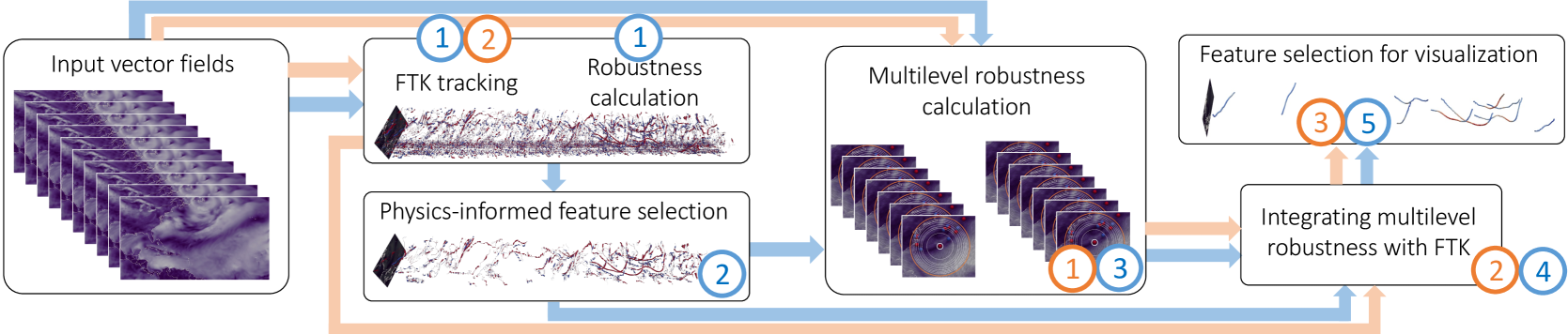
As shown in Fig. 4 (orange arrows and indices), the implementation of MRT framework involves the following three steps:
Step 1: multilevel robustness calculation. The MRT framework calculates the multilevel robustness for all detected critical points with evenly increased radii until the neighborhood includes the entire input domain. Then, the minimum multilevel robustness is calculation for postprocessing.
Step 2: integration with feature tracking. The MRT framework integrates the minimum multilevel robustness with FTK [17] to enhance the original FTK tracking results.
Step 3: feature selection. The MRT framework utilizes two filters based on multilevel robustness and degree information of tracks for feature selection. These feature selection strategies can help users reduce visual clutter and highlight dominant features in the domain.
TROPHY reuses the notion of multilevel robustness, described in Section 2.2.1, and the method to integrate the minimum multilevel robustness with FTK; see Section 2.2.2. In the following section, we customize the MRT framework to TROPHY by integrating the physical knowledge of TCs in feature extraction and tracking.
3 Method: TROPHY for Cyclone Tracking
Our physics-informed tracking framework, TROPHY, encodes several criteria considering the physical properties of cyclones. These criteria make TROPHY more efficient and appropriate for cyclone tracking than the MRT framework.
Overview of TROPHY. An overview of our pipeline is shown in Fig. 4. First, we compute the FTK tracking result for the whole dataset and the classic robustness of the critical points using the entire domain for each time step. Second, the FTK tracks and the robustness of critical points are used in the physics-informed feature selection (Section 3.1) to filter out noise-liked tracks. Third, an adaptive-level strategy (Section 3.2) is applied in the multilevel robustness calculation for selected critical points. Fourth, TROPHY integrates the minimum multilevel robustness with FTK to enhance the original FTK tracking results. This step uses the same strategy with the MRT framework; see Section 2.2.2 or [53, Sect. 5.1] for a detailed discussion. Finally, we utilize one stability filter function from [53] and propose two additional physics-informed filter functions to highlight cyclones; see Section 3.3.
3.1 Physics-Informed Feature Selection
We now introduce a physics-informed feature selection strategy during preprocessing, making TROPHY much more efficient than the MRT framework in studying large-scale datasets. The MRT framework computes multilevel robustness for all detected critical points. For the example in Fig. 3 (A), 102,720 critical points and 22,743 tracks are detected with FTK. Suppose we set the number of levels , the MRT framework needs to conduct times classic robustness computation. TROPHY instead focuses on tracking cyclone-liked features, which selects a subset of critical points/tracks for in-processing. Considering the physical properties of real-world cyclones, we incorporate two criteria in physics-informed feature selection before multilevel robustness calculations.
First, since the duration of a tropical storm/cyclone is usually larger than 1 day, we require the selected tracks to contain at least one 1-day segment that consists of degree critical points only.
Second, since a critical point representing the center of a cyclone usually has a high stability measure across time before it hits the land and dissipates, we require the segment detected from the previous step to have a high average robustness value. Based on domain knowledge, a tropical storm must have maximum sustained winds of at least 17.5 m/s. We set the threshold to 1.75 for track filtering.
With these two requirements, the numbers of critical points and tracks decrease to 9,784 and 86, respectively; compare Fig. 3 (A) and (B). Thus, TROPHY needs to compute multilevel robustness for only of critical points compared with the original MRT framework.

3.2 Adaptive Levels for Multilevel Robustness
We next propose an adaptive level strategy for the multilevel robustness calculation. Such a strategy also considers physical properties of real-world cyclones and leads to more reasonable minimum multilevel robustness values for TROPHY than does the MRT framework. As discussed in Section 2.2.1, the MRT framework approximates the exact multilevel robustness with a set of evenly spaced radii. This strategy may lead to two consequences that are counterintuitive in real-world cyclone analysis. First, a critical point can be canceled with other critical points that are far away in the known data domain due to boundary effects; see partners for and in Fig. 2 (A) and (B). Although such cancellations are mathematically justifiable, it is almost impossible to happen in real-world scenarios since no perturbation could happen across the whole Atlantic Ocean. Second, the MRT framework may not find the true minimum multilevel robustness value due to sampling. It may also waste computational resources when an enlarged neighborhood does not include potential cancellation partners. For example, increasing the radius of the neighborhood from 60 to 80 for in Fig. 2 (C) does not lead to new cancellation candidates.
To mitigate the drawbacks of the MRT framework, we introduce an adaptive-level strategy. First, we set a physics-informed neighborhood size, where real-world perturbation could happen. We set this radius to be 10 degrees since hurricanes are among the most destructive real-world perturbations to wind field and are typically about 4.7 degrees wide. The TROPHY considers all possible cancellation partners within this neighborhood using varying radii. Fig. 5 (A) illustrates our adaptive level strategy in calculating the multilevel robustness. For a critical point , we consider all critical points within its neighborhood at radius 10. Suppose there are () critical points in this neighborhood and their Euclidean distances to are . We compute the classic robustness of within neighborhood defined by these radii, giving rise to its multilevel robustness. If , we select an additional closest critical points outside of the selected neighborhood for more candidates of cancellation partners; see Fig. 5 (B). However, in most cases, the cancellation partners for the true minimum multilevel robustness are located in our physics-informed neighborhood, for example, degree for , degree for , and degree for in Fig. 2.

3.3 TC Feature Selection for Visualization
We now present feature selection aided by the minimum multilevel robustness and physical properties of TCs. We inherit one stability filter from the MRT framework. This filter considers the minimum multilevel robustness and its temporal stability in terms of lifespan. Let denote a logistic transformation of , which maps the to . This normalization is defined as
where is the logistic growth rate; see [53, Sect. 5.1] for a detailed discussion on the benefit of this normalization and parameter selection for . Now let denote a track, is its total length. The stability of a track is defined as
| (1) |
where is the temporal span of the input dataset and is the temporal span of . The first term in Eq. (1) captures the average pointwise stability (in a logistic scale), whereas the second term encodes the lifespan of the track. By definition, .
Our second feature selection strategy is referred to as maximum wind speed (MWS) filter. Since the storm systems are usually categorized by the Saffir–Simpson Hurricane Wind Scale, which considers only a hurricane’s maximum sustained wind speed, we use this filter to control the categories of storm that users want to visualize. Formally, for a track , its maximum wind speed is
| (2) |
where is the MWS within the two-degree region of the center .
Our third feature selection strategy is referred to as smoothness filter. It is used to filter out tracks that are too tortuous to be considered as TC tracks. Roughly speaking, we define the smoothness of a track by the average distance between the normalized track and its smooth univariate spline. Formally, for a track , its smoothness is
| (3) |
where is a normalization term mapping to and maps to the point on the smooth univariate spline of the normalized . TROPHY uses the SciPy Python library to calculate the (degree 3) smooth univariate splines for detected tracks. Fig. 6 shows three curves from our climate dataset and their smooth univariate splines. The left track has the lowest average distance and hence the highest smoothness value, whereas the right track has the lowest smoothness value and usually cannot be considered as a TC track.

In Fig. 7, we apply the above three filters to the dataset (see Sections 4 and C for details). After integrating multilevel robustness with FTK tracking results, we obtain tracks in Fig. 7 (A), which still suffer from visual clutter. By applying the stability filter with a threshold of for , we obtain tracks in Fig. 7 (B). If we keep enlarging the stability threshold, track will be filtered out before track , even if track represents the Category 1 hurricane Otto, and track cannot be found in the National Hurricane Center’s Tropical Cyclone Reports. Therefore, we use our MSF filter based on the MSF along the track and set the threshold to be . The remaining tracks are shown in Fig. 7 (D). Again, if we keep increasing the threshold for , track will be filtered out before track , whereas track represents the Category 1 hurricane Lisa. Therefore, we apply our third smoothness filter in Fig. 7 (E) and (F). Now, TROPHY highlights 8 tracks representing hurricanes/tropical storms that can all be found in the National Hurricane Center’s Tropical Cyclone Reports.
4 Metrics, Data, and Methods for Evaluation
We present experimental results using using 30-year (1981–2010) near-surface wind vector field from the ECMWF Reanalysis v5 (ERA5). We annotate this 30-year dataset as the dataset. We also mark the one-year subset data from the dataset as . We use the International Best Track Archive for Climate Stewardship (IBTrACS [26] version 4) observations as the reference and the TC tracking results of the TempestExtremes software package [44] for comparision. The details of datasets, IBTrACS, and TempestExtremes are described in Appendix C. We now describe the metrics used for evaluating the performance of TROPHY in Section 4.1. We also discuss the parameter tuning for TROPHY in Section 4.2.
4.1 Metrics for Evaluating Tropical Cyclones
We review several metrics used for evaluating TCs in climate data. See [56] for detailed descriptions.

4.1.1 Storm Climatology and Characteristics
Annual frequency, marked as count or (#), is measured by the number of discrete storm events.
Annual duration, marked as (days), can be defined as , where is occurrence of 6 hourly-tracked points during the lifetime of storm .
Storm genesis, marked as gen, is defined as the first entry for each individual storm’s lifetime.
Storm intensity can be measured by the minimum sea level pressure at the cyclone center, marked as SLP (hPa), and two-degree maximum 10-meter wind speed, marked as ().
Latitude of lifetime-maximum intensity, marked as LMI, is defined as the absolute value of the latitude where a TC reaches its maximum intensity (as defined by maximum ).
4.1.2 Statistics
We employ two statistical techniques to evaluate the above metrics on a 30-year (1981–2010) dataset.
One is the arithmetic mean, , which is used in Section 5.4 to study annual domain-averaged climatology.
The second is the Pearson correlation coefficient , defined as
which is used in Section 5.5 to evaluate the similarity of metrics w.r.t. temporal (e.g., storm frequency) or spatial (e.g., genesis density) patterns, which are generated by TC tracking results from the tested tracking algorithm and reference observations.
4.2 Configuration for Feature Selection
For filters introduced in Section 3.3, we recommend a default value as a threshold for each filter function based on the TC tracks provided by IBTrACS. First, we calculate the spatial pattern of cumulative track density using TC tracks detected by TROPHY with thresholds of stability varying from 0.02 to 0.035, MWS varying from 10 to 14, and smoothness varying from 0.95 to 0.97. We also calculate the spatial pattern of cumulative track density from IBTrACS as a baseline. Then, we evaluate the similarity between the density patterns from TROPHY and IBTrACS using Pearson correlation, marked as , which is the most exhaustive measure of TC activity. We provide a detailed example for computation in Section 5.5. We suggest the thresholds for , , and with the values when reaches its maximum, that is, 0.029 for stability , 13.5 for MWS , and 0.967 for smoothness . TROPHY also allows users to fine-tune these thresholds independently for individual TC tracks of interest. We report performances of TROPHY with both default thresholds and human-in-the-loop thresholds in Section 5. We demonstrate that, although the tracking results using default threshold are encouraging, results with the human-in-the-loop option can further improve the performance of TROPHY.
5 Cyclone Tracking Results With TROPHY
We demonstrate cyclone-tracking results using TROPHY and their comparisons with a state-of-the-art TC tracking algorithm. Observations from official forecast centers are provided for reference.


5.1 Overview of Results
We apply TROPHY to the dataset on a cluster with 664 nodes (128GB DDR4 and 36 cores per node). We utilize the method of Tricoche et al. [41] to calculate degrees of critical points for the vector field in each time step and parallelize the computation of multilevel robustness with Eden [32], which can schedule and manage a number of tasks on a high-performance computing cluster.
Even though we have obtained the tracking results using TROPHY for all 30 years of data, we demonstrate TC tracking results for 1981, 1990, 2004, and 2009 in Fig. 8 to highlight the tracking differences between various datasets and algorithms. TempestExtremes tracks TC eyes as positions with the local minimum SLP, whereas the TC eyes from TROPHY are located where wind speeds are zeros. Therefore, TC tracks from TempestExtremes and TROPHY do not overlap exactly. Both methods consider the area within a two-degree great circle of a detected TC eye to find a local maximum and use it to measure storm intensity [55, 44]. Tracks in Figs. 8, 9 and 10 are colored by storm intensity w.r.t. this two-degree maximum wind speed, referred to as wind speed for simplicity. We discuss some preliminary findings based on Fig. 8 in the following paragraphs
First, since TempestExtremes requires both dynamic and thermodynamic variables to meet its specified criteria, it usually cannot detect the beginnings and endings of TC where wind speeds are low. TROPHY can detect such tails as long as the centers of flows can be identified as critical points; see tracks , , and in Fig. 8.
Second, TROPHY can detect some discrete storm events that are not captured by TempestExtremes, such as tracks and in Fig. 8. Track can be found in IBTrACS, whereas track cannot. To further investigate these discrepancies, including tracks that cannot be captured by TempestExtremes/IBTrACS but are found by TROPHY, and tracks that are in IBTrACS but are undetected by TROPHY, we conducted case studies (reported in Sections 5.2 and 5.3).
Third, using fine-tuned filter thresholds for TROPHY, we can get TC tracking results that are more similar to IBTrACS. For example, track is missed by TROPHY with a default threshold for smoothness, since is severely bent and has a relatively low smoothness value. When, however, we decrease the threshold for from 0.967 to 0.95, track is shown in the TC tracking result as indicated by the red arrow in Fig. 8. Similarly, track , which is not recorded in IBTrACS, can be filtered out if we increase the threshold of stability from 0.029 to 0.03. These sensitivities to parameters in the tracking algorithm are, in general, expected [15]. This human-in-the-loop option provides users the opportunity of fine-tuning, especially for short-term forecasting or weather-scale studies, as accuracy is more important at this scale. At the climate scale and for climate change impacts, users may use the same thresholds for all TC cases in both historic and future periods, to avoid the impacts of parameter uncertainties.
5.2 Case Study: Tracking TC during Dissipation
We now investigate a Category 2 hurricane track named Hurricane Bonnie. As illustrated in Fig. 9, (A) shows the TC tracks from TempestExtremes (colored by wind speed) and IBTrACS (in black), whereas (B) shows the TC tracks detected by TROPHY. We observe a much longer tail in (B) with low wind speed compared with (A). (C) gives the zoomed-in views of tails of TC tracks detected by TempestExtremes (1st row) and TROPHY (2nd row). Vector fields from different time steps are shown as background. We also highlight the TC eyes detected by each method in corresponding time steps by arrows on (C). We see TC eyes detected by TROPHY are exactly located where the wind vanishes, whereas the TC eyes from TempestExtremes are slightly shifted to the outside of the eyes. The last two columns of (C) show that TROPHY can track the TC eyes during dissipation because the wind flow is still spinning even if the wind speed is low. TROPHY tracks such flow behaviors as sources until the sources disappear.
5.3 Case Study: Terminating Tracking
We next investigate a Category 1 hurricane named Hurricane Lisa, which is captured by TempestExtremes but is partially missed by TROPHY. Fig. 10 (A–C) show TCs of 1998, which are recorded in IBTrACS and detected by TempestExtremes and TROPHY with the dataset, respectively. We focus on the analysis of Hurricane Lisa, marked as , , and in different methods. We note that , detected by TROPHY, has a clearly shorter track compared with the other two datasets because the eyes of Hurricane Lisa were detected as centers only up to 10/08/1998 00:00 AM, after which Hurricane Lisa lost its distinct eye and could not be detected by TROPHY; see Fig. 10 (M), as well as a zoomed-in view in Fig. 10 (d).
Such a process could be related to TC’s extratropical transitions [25], which may occur as Hurricane Lisa moves over cooler water and into areas of stronger wind shear at higher latitudes. During this transition, the cyclone loses its symmetric and distinct eye and, thus, TROPHY terminates its tracking.
In fact, Hurricane Lisa produced distinct eyes again at time step 10/09/1998 at 12:00 PM and 10/10/1998 at 00:00 AM, so TROPHY was able to start the track again. However, because these tracks were short-lived, they were filtered out during the initial feature selection.
5.4 Evaluations: Annual Domain-Averaged Climatology
This section and the following present the evaluations of TROPHY using the metrics described in Section 4.1. For annual climatology, cumulative statistics are calculated over the entire data period (30 years), which are then normalized to a per-year basis. Table 1 shows annually averaged statistics for TCs detected by TROPHY and TempestExtremes.
| () | |||
|---|---|---|---|
| IBTrACS | 10.74 | 79.34 | 25.65 |
| TempestExtremes | 8.17 | 50.01 | 38.30 |
| TROPHY (default) | 5.3 | 52.62 | 31.55 |
| TROPHY (human-in-loop) | 7.77 | 66.43 | 29.98 |
According to annual TC count (), IBTrACS contains approximately 11 TCs per year within the studied region, whereas TROPHY with default setting produces the least number of TCs. However, when considering annual storm lifetime (i.e., ), TROPHY detects longer storms than TempestExtremes and is closer to IBTrACS on average. This result is consistent with what we observed in our experiments. TROPHY can detect TCs not only during their movements but also, at least partially, during their formation and dissipation periods, even if their wind speed is low; see Fig. 9 for an example. Also, since TempestExtremes requires dynamic and thermodynamic variables to meet specified criteria, TC tracks may break into pieces when some parts of the track do not meet the requirement; see the track indicated by a purple circle from Fig. 8 for an example. Overall, TROPHY produces TC tracks for a longer time than does TempestExtremes, whereas TempestExtremes detects more TC tracks than does TROPHY.
In addition, although TROPHY’s TC tracks have closer hurricane genesis w.r.t. the observation, both TROPHY and TempestExtremes show a poleward bias compared with IBTrACS’s genesis. One of the reasons for this bias could be that the reanalysis data including ERA5 are not able to simulate storm structures near the equator well, according to Knaff et al. [25], indicating that the input data to any tracking algorithms is the most important factor when studying TCs.
5.5 Evaluations: Spatial Climatology
For spatial pattern climatology, density maps are generated by aggregating occurrences into by bins. An example of the spatial track density patterns is shown in Fig. 11. The spatical correlation between IBTrACS and TROPHY (default) is caculated using patterns from Fig. 11 (A) and (C). To quantify the similarity between IBTrACS and TROPHY (or TempeExtremes), we calculate Pearson correlation coefficient for total occurrence (), genesis occurrence (), maximum wind speed, and minimum SLP. Table 2 shows the pattern correlation of TROPHY/TempestExtremes with observations.
Both TROPHY and TempestExtremes can produce reasonable distributions of storm occurrence when compared with observations (). The spatial patterns of genesis () from TROPHY and TempestExtremes show lower correlations () with observations. This is not surprising because the initialization and development of a clear eye depend on many other factors such as their 3D evolutions, which are beyond the capability of what our 2D vector fields can represent. In fact, predicting the genesis of TC is one of the scientific challenges in TC research fields, indicating that the currently available data cannot capture TC genesis and that new frameworks of such calculations are needed [54]. Both TROPHY and TempestExtremes are able to produce storm strength similar to that of observations () in terms of maximum and minimum sea level pressure.

| IBTrACS | 1.00 | 1.00 | 1.00 | 1.00 |
| TempestExtremes | 0.892 | 0.638 | 0.920 | 0.889 |
| TROPHY (default) | 0.897 | 0.569 | 0.925 | 0.901 |
| TROPHY (human-in-loop) | 0.914 | 0.634 | 0.933 | 0.920 |
6 Conclusion and Discussion
We introduce a physics-informed TC tracking framework, TROPHY, that utilizes tools from vector field topology. Based only on a 2D wind vector field, TROPHY is able to produce results comparable to (and sometimes even better than) those obtained with a widely used TC tracking algorithm—TempestExtremes—while requiring far less input data. Although TROPHY does not consider the air temperature field (e.g., the warm cores) of TCs, the symmetric eye structures of TCs allow TROPHY to detect and track them. Furthermore, our framework may be used in uncertainty visualization to understand uncertainty due to different model physics or setup, or feature comparison of geoscientific data with space and time dimensions.
TROPHY has a number of limitations. First, our robustness-based framework is very useful for hurricane tracking, since hurricanes have symmetric structures and hurricane tracks are one of the most important factors in assessing their risks. However, once the symmetric structures (i.e., the eyes) are weakened or disappear with the cyclones moving to higher latitudes, TROPHY does not consider them as TCs anymore. This is because the cyclone at higher latitudes may get their energy from one or more front systems dividing warm air from the south and cold air front the north, see Fig. 10. Such frontal systems lead to asymmetric structures, which are not detected by TROPHY. In general, our technique may not be suitable for asymmetric feature tracking such as extratropical cyclones. Second, to obtain optimal tracking results, we may need to fine-tune the parameters for each single event. Third, the current framework only considers the near surface (10 meters) winds. However, higher altitude winds (dozens to hundreds of meters) are also big concerns when it comes to real-world applications such as wind energy. This is left for future work.
From an application perspective, to the best of our knowledge, it is an open challenge to incorporate 3D data in the study of TCs, based on domain scientist feedback. Because adding more variables may reduce the overall efficiencies of TROPHY yet may not guarantee a better performance. From an algorithmic perspective, it may be possible to extend TROPHY to utilize 3D data for TC tracking. First, we may use horizontal layers of a 3D vector field along the vertical direction. Second, we may utilize a third variable called the vertical motion (i.e., upward and downward), in addition to zonal wind (U) and meridional (V) wind. Expanding TROPHY to either of these directions could be useful in better detecting, tracking and understanding hurricanes such as their genesis, intensification, and landfall (important factors to be considered for risk assessment). The robustness framework has been extended previously to study 2D symmetric tensor fields [47, 22] and critical points in 3D vector fields [34]. It may be feasible to integrate the robustness framework for 3D critical points in TROPHY. However, there are more complex features that need to be considered in 3D, such as vortex regions or vortex core lines. We would need to develop theoretical foundations to quantify their robustness first before establishing their physical interpretability in studying TCs.
Acknowledgements.
This study is supported by the Wind Energy Technologies Office of the DOE. Argonne National Laboratory is a US Department of Energy laboratory managed by UChicago Argonne, LLC, under contract DE-AC02-06CH11357. This research was also supported by DOE DE-SC0022753, DOE DE-SC0023193, DOE DE-SC0021015, NSF IIS 2145499, NSF IIS 1910733, and DOE DE-AC02-06CH11357.References
- [1] Copernicus Climate Change Service. https://climate.copernicus.eu/.
- [2] S. S. Bell, S. S. Chand, K. J. Tory, and C. Turville. Statistical assessment of the OWZ tropical cyclone tracking scheme in ERA-Interim. Journal of Climate, 31(6):2217–2232, 2018.
- [3] M. Biswas, L. Bernardet, S. Abarca, I. Ginis, E. Grell, E. Kalina, Y. Kwon, B. Liu, Q. Liu, T. Marchok, et al. Hurricane weather research and forecasting (hwrf) model: 2018 scientific documentation. Developmental Testbed Center, p. 112, 2018.
- [4] K. G. Blackwell. The evolution of Hurricane Danny (1997) at landfall: Doppler-observed eyewall replacement, vortex contraction/intensification, and low-level wind maxima. Monthly Weather Review, 128(12):4002–4016, 2000.
- [5] S. Bourdin, S. Fromang, W. Dulac, J. Cattiaux, and F. Chauvin. Intercomparison of four tropical cyclones detection algorithms on ERA5. 2022.
- [6] P.-T. Bremer, G. Weber, J. Tierny, V. Pascucci, M. Day, and J. Bell. Interactive exploration and analysis of large-scale simulations using topology-based data segmentation. IEEE Transactions on Visualization and Computer Graphics, 17(9):1307–1324, 2010.
- [7] R. Bujack, L. Yan, I. Hotz, C. Garth, and B. Wang. State of the art in time-dependent flow topology: Interpreting physical meaningfulness through mathematical properties. Computer Graphics Forum, 39(3):811–835, 2020.
- [8] B. Cabral and L. C. Leedom. Imaging vector fields using line integral convolution. In Proceedings of the 20th Annual Conference on Computer Graphics and Interactive Techniques, SIGGRAPH ’93, pp. 263–270. Association for Computing Machinery, New York, NY, USA, 1993. doi: 10 . 1145/166117 . 166151
- [9] S. J. Camargo and S. E. Zebiak. Improving the detection and tracking of tropical cyclones in atmospheric general circulation models. Weather and forecasting, 17(6):1152–1162, 2002.
- [10] P.-L. Chang, B. J.-D. Jou, and J. Zhang. An algorithm for tracking eyes of tropical cyclones. Weather and forecasting, 24(1):245–261, 2009.
- [11] H. Doraiswamy, V. Natarajan, and R. S. Nanjundiah. An exploration framework to identify and track movement of cloud systems. IEEE Transactions on Visualization and Computer Graphics, 19(12):2896–2905, 2013.
- [12] H. Edelsbrunner, J. Harer, A. Mascarenhas, and V. Pascucci. Time-varying Reeb graphs for continuous space-time data. In Proceedings of the twentieth annual symposium on Computational geometry, pp. 366–372, 2004.
- [13] W. Engelke, T. B. Masood, J. Beran, R. Caballero, and I. Hotz. Topology-based feature design and tracking for multi-center cyclones. arXiv preprint arXiv:2011.08676, 2020.
- [14] B. M. Enz, J. P. Engelmann, and U. Lohmann. Parallel use of threshold parameter variation for tropical cyclone tracking. Geoscientific Model Development Discussions, 2022:1–29, 2022. doi: 10 . 5194/gmd-2022-279
- [15] B. M. Enz, J. P. Engelmann, and U. Lohmann. Parallel use of threshold parameter variation for tropical cyclone tracking. Geoscientific Model Development Discussions, pp. 1–29, 2022.
- [16] C. Garth, X. Tricoche, and G. Scheuermann. Tracking of vector field singularities in unstructured 3D time-dependent datasets. In Proceedings of IEEE Visualization 2004, pp. 329–336. IEEE, Austin, TX, USA, 2004.
- [17] H. Guo, D. Lenz, J. Xu, X. Liang, W. He, I. R. Grindeanu, H.-W. Shen, T. Peterka, T. Munson, and I. Foster. FTK: a simplicial spacetime meshing framework for robust and scalable feature tracking. IEEE Transactions on Visualization and Computer Graphics, 27(8):3463–3480, 2021. doi: 10 . 1109/TVCG . 2021 . 3073399
- [18] J. Helman and L. Hesselink. Representation and display of vector field topology in fluid flow data sets. IEEE Computer Architecture Letters, 22(08):27–36, 1989.
- [19] J. L. Helman and L. Hesselink. Surface representations of two-and three-dimensional fluid flow topology. In Proceedings of the First IEEE Conference on Visualization: Visualization90, pp. 6–13. IEEE, 1990.
- [20] K. Hodges, A. Cobb, and P. L. Vidale. How well are tropical cyclones represented in reanalysis datasets? Journal of Climate, 30(14):5243–5264, 2017.
- [21] G. Holland and C. L. Bruyère. Recent intense hurricane response to global climate change. Climate Dynamics, 42:617–627, 2014.
- [22] J. Jankowai, B. Wang, and I. Hotz. Robust extraction and simplification of 2D tensor field topology. Computer Graphics Forum (CGF), 38(3):337–349, 2019.
- [23] J. D. Kepert. Objective analysis of tropical cyclone location and motion from high-density observations. Monthly Weather Review, 133(8):2406–2421, 2005.
- [24] S. Kleppek, V. Muccione, C. C. Raible, D. N. Bresch, P. Koellner-Heck, and T. F. Stocker. Tropical cyclones in ERA-40: a detection and tracking method. Geophysical Research Letters, 35(10), 2008.
- [25] J. A. Knaff, S. P. Longmore, and D. A. Molenar. An objective satellite-based tropical cyclone size climatology. Journal of Climate, 27(1):455–476, 2014. doi: 10 . 1175/JCLI-D-13-00096 . 1
- [26] K. R. Knapp, M. C. Kruk, D. H. Levinson, H. J. Diamond, and C. J. Neumann. The International Best Track Archive for Climate Stewardship (IBTrACS): Unifying tropical cyclone data. Bulletin of the American Meteorological Society, 91(3):363–376, 2010. doi: 10 . 1175/2009BAMS2755 . 1
- [27] J. P. Kossin, T. L. Olander, and K. R. Knapp. Trend analysis with a new global record of tropical cyclone intensity. Journal of Climate, 26(24):9960–9976, 2013.
- [28] W.-C. Lee and F. D. Marks. Tropical cyclone kinematic structure retrieved from single-doppler radar observations. Part II: The GBVTD-simplex center finding algorithm. Monthly Weather Review, 128(6):1925–1936, 2000.
- [29] T. Marchok. Important factors in the tracking of tropical cyclones in operational models. Journal of Applied Meteorology and Climatology, 60(9):1265–1284, 2021.
- [30] E. Nilsson, W. Engelke, A. Friederici, and I. Hotz. Tracking and visualizing multi-center cyclones. In Levia, 2020.
- [31] J. Reininghaus, J. Kasten, T. Weinkauf, and I. Hotz. Efficient computation of combinatorial feature flow fields. IEEE Transactions on Visualization and Computer Graphics, 18(9):1563–1573, 2012.
- [32] S. Simmerman, J. Osborne, and J. Huang. Eden: Simplified management of atypical high-performance computing jobs. Computing in Science & Engineering, 15(6):46–54, 2012.
- [33] M. Sivaramakrishnan and M. Selvam. On the use of the spiral overlay technique for estimating the center positions of tropical cyclones from satellite photographs taken over the Indian region. In Proceedings of the 12th conference on Radar Meteorology, pp. 440–446. Norman, OK, USA, 1966.
- [34] P. Skraba, P. Rosen, B. Wang, G. Chen, H. Bhatia, and V. Pascucci. Critical point cancellation in 3D vector fields: Robustness and discussion. IEEE Transactions on Visualization and Computer Graphics, 22(6):1683–1693, 2016.
- [35] P. Skraba and B. Wang. Interpreting feature tracking through the lens of robustness. In P.-T. Bremer, I. Hotz, V. Pascucci, and R. Peikert, eds., Topological Methods in Data Analysis and Visualization III: Theory, Algorithms, and Applications (Proceedings of TopoInVis 2013), pp. 19–38. Springer, 2014.
- [36] P. Skraba, B. Wang, G. Chen, and P. Rosen. 2D vector field simplification based on robustness. In 2014 IEEE Pacific Visualization Symposium, pp. 49–56. Yokohama, Japan, 2014.
- [37] P. Skraba, B. Wang, G. Chen, and P. Rosen. Robustness-based simplification of 2D steady and unsteady vector fields. IEEE Transactions on Visualization and Computer Graphics, 21(8):930–944, 2015.
- [38] B.-S. Sohn and C. Bajaj. Time-varying contour topology. IEEE Transactions on Visualization and Computer Graphics, 12(1):14–25, 2005.
- [39] A. A. Taylor and B. Glahn. Probabilistic guidance for hurricane storm surge. In 19th Conference on probability and statistics, vol. 74, 2008.
- [40] H. Theisel and H.-P. Seidel. Feature flow fields. In Proceedings of the symposium on Data visualisation 2003, pp. 141–148. Grenoble, France, 2003.
- [41] X. Tricoche, G. Scheuermann, and H. Hagen. Continuous topology simplification of planar vector fields. In Proceedings of Visualization, 2001. VIS’01., pp. 159–166. IEEE, San Diego, CA, USA, 2001.
- [42] X. Tricoche, G. Scheuermann, and H. Hagen. Topology-based visualization of time-dependent 2D vector fields. In Data Visualization 2001, pp. 117–126. Springer, 2001.
- [43] X. Tricoche, T. Wischgoll, G. Scheuermann, and H. Hagen. Topology tracking for the visualization of time-dependent two-dimensional flows. Computers & Graphics, 26(2):249–257, 2002.
- [44] P. A. Ullrich and C. M. Zarzycki. TempestExtremes: a framework for scale-insensitive pointwise feature tracking on unstructured grids. Geoscientific Model Development, 10(3):1069–1090, 2017. doi: 10 . 5194/gmd-10-1069-2017
- [45] K. J. Walsh, J. L. McBride, P. J. Klotzbach, S. Balachandran, S. J. Camargo, G. Holland, T. R. Knutson, J. P. Kossin, T.-c. Lee, A. Sobel, et al. Tropical cyclones and climate change. Wiley Interdisciplinary Reviews: Climate Change, 7(1):65–89, 2016.
- [46] B. Wang, R. Bujack, P. Rosen, P. Skraba, H. Bhatia, and H. Hagen. Interpreting Galilean invariant vector field analysis via extended robustness. In Topological Methods in Data Analysis and Visualization, pp. 221–235. Springer, 2017.
- [47] B. Wang and I. Hotz. Robustness for 2D symmetric tensor field topology. In T. Schultz, E. Özarslan, and I. Hotz, eds., Modeling, Analysis, and Visualization of Anisotropy, pp. 3–27. Springer International Publishing, 2017.
- [48] B. Wang, P. Rosen, P. Skraba, H. Bhatia, and V. Pascucci. Visualizing robustness of critical points for 2D time-varying vector fields. Computer Graphics Forum, 32(3pt2):221–230, 2013. doi: 10 . 1111/cgf . 12109
- [49] T. Weinkauf, H. Theisel, A. Van Gelder, and A. Pang. Stable feature flow fields. IEEE Transactions on Visualization and Computer Graphics, 17(6):770–780, 2010.
- [50] H. Willoughby. Tropical cyclone eye thermodynamics. Monthly Weather Review, 126(12):3053–3067, 1998.
- [51] T. Wischgoll and G. Scheuermann. Detection and visualization of closed streamlines in planar flows. IEEE Transactions on Visualization and Computer Graphics, 7(2):165–172, 2001.
- [52] K. Y. Wong, C. L. Yip, and P. W. Li. Automatic tropical cyclone eye fix using genetic algorithm. Expert Systems with Applications, 34(1):643–656, 2008.
- [53] L. Yan, P. A. Ullrich, L. P. Van Roekel, B. Wang, and H. Guo. Multilevel robustness for 2D vector field feature tracking, selection, and comparison. Computer Graphics Forum, accepted (see also arXiv preprint arXiv:2209.11708), 2023.
- [54] W. Yang, T.-L. Hsieh, and G. A. Vecchi. Hurricane annual cycle controlled by both seeds and genesis probability. Proceedings of the National Academy of Sciences, 118(41):e2108397118, 2021.
- [55] C. M. Zarzycki and P. A. Ullrich. Assessing sensitivities in algorithmic detection of tropical cyclones in climate data. Geophysical Research Letters, 44(2):1141–1149, 2017.
- [56] C. M. Zarzycki, P. A. Ullrich, and K. A. Reed. Metrics for evaluating tropical cyclones in climate data. Journal of Applied Meteorology and Climatology, 60(5):643–660, 2021.
Appendix A An Example of Merge Tree
We now give an example of an augmented merge tree that is constructed from the dataset. First, we define a scalar field by assigning the vector magnitude to each point , that is, ; see Fig. 12(A) and (B), which visualize the vector field and scalar field . Second, we track the merging behavior of components that contain critical points of . For example, the component containing and merges with the component containing at and forms in , which is represented by the purple and green region in Fig. 12 (D). Third, we augment the merge tree with the degrees of critical points (on leaves) and the degrees of components (on internal nodes). For example, component in Fig. 12 (D) contains critical points and , whose degrees are and , respectively. The degree of is , i.e., . The augmented merge tree of Fig. 12 (A) is shown in Fig. 12 (E).
Appendix B An Example of Robustness Calculation
Using the example in Fig. 12 (A)-(E), we now show how to calculate robustness with an augmented merge tree. As pointed out in Section 2.1, the robustness of a critical point can be calculated as the function value of its lowest zero-degree ancestor in the augmented merge tree. The robustness of and is 0.65, whereas the robustness of and is 14.7. Intuitively, for the example in Fig. 12 (A)-(E), it is easier for and to be canceled with each other than and , since they have much lower robustness values. In Fig. 12 (F), we give the vector field from the same dataset but one time step (6 hours) behind the vector field of Fig. 12 (A). We see and disappear, whereas and remain.

Appendix C Details on Dataset and Methods
We demonstrate the performance of TROPHY using 30-year (1981–2010) near-surface wind vector field from the ECMWF Reanalysis v5 (ERA5). It is produced by the Copernicus Climate Change Service (C3S) [1]. ERA5 provides hourly estimates of the global climate information with a spatial grid resolution of 30 km. Since tropical cyclones/storms usually occur during June and October, we limit our dataset with a time window from June to October every year at standard synoptic reporting times (0000, 0600, 1200, and 1800 UTC). A rectangle region on the Atlantic Ocean ( N∘ to N∘ and W∘ to W∘) is selected. We utilize 10-meter zonal and meridional wind speed as the 2D vector field, since in the near-surface the hurricane core represents a region of strong convergence and associated vertical motion. We annotate this 30-year dataset as the dataset. We also mark the one-year subset data from the dataset as ; for example, Fig. 3 uses the dataset.
We use the International Best Track Archive for Climate Stewardship (IBTrACS [26] version 4) observations as the reference. IBTrACS is compiled from quality-controlled records from various forecasting centers. In this paper, we select TCs reported by World Meteorological Organization (WMO) official forecast centers. Again, only tropical cyclones/storms within the region of the dataset are visualized. For comparison purposes, we include the TC tracking results of the TempestExtremes software package [44] applied to the dataset with the parameter setting following [55].