Triplet pairing, orbital selectivity and correlations in iron-based superconductors
Abstract
We use a slave-boson approach to study the band renormalization and pair susceptibility in the normal state of iron-based superconductors in presence of strong Coulomb repulsion and Hund’s interaction. Our results show orbital selectivity toward localization of orbitals and its interplay with superconductivity. We also compare the recently proposed triplet resonating valence bond theory of superconductivity in Iron based superconductors with the more conventional pairing and show that both favor a superconductivity when the orbital is delocalized.
I Introduction
A major open question in the theory of strongly correlated electronic systems is the origin of the superconductivity in iron-based superconductors (FeSC) [1]. Since their discovery more than a decade ago, a large body of data has been collected which has largely been interpreted in the framework of singlet superconductivity [2, 3]. A widely accepted paradigm for the pairing in these materials, based on itinerant electrons in the presence of an attractive pairing glue [4, 5] that binds them into Cooper pairs, has been successful in explaining a subset of this data. There is, however, less consensus on the origin of the pairing glue. Various exchange bosons have been suggested, from spin, nematic and orbital fluctuations to a combination thereof [6, 7]. At the same time, as we expand upon below, a variety of new experimental data has shown signatures of an interplay between complex orbital and local moment physics [8] with superconductivity. The consistency of these findings with the paradigm of electrons subject to a fluctuation-mediated pairing glue is currently unclear.
Considering the complexity of this multi-orbital system and presence of many competing orders and putative critical points, the pursuit of a single origin for the superconductivity may be fraught with difficulty. A more modest goal is to seek the minimal ingredients for superconductivity in FeSC. In a recent paper [9] we suggested that Hund’s coupling is a the driver [10] of the superconductivity, giving rise to an orbitally-odd spin-triplet superconductor. Although itinerant triplet pairing in iron-based SC was discussed early on by Wen and Lee [11] this idea was quickly dismissed due to the observation of a Knight shift and the absence of nodes on the Fermi surface (FS). Triplet pairing in iron-based superconductors has recently been re-visited [12, 13, 14, 15] in the context of a possible interplay between pairing and the topological bandstructure.
Given the pre-dominant support for an singlet pairing scenario, it is instructive to re-iterate the motivation for a triplet state. Dynamical mean-field theory (DMFT) [16] has long shown that the Hund’s interaction plays a dominant role in the correlations of the normal state [17, 18, 19, 20, 21, 22], a picture that is also confirmed in slave-spin mean-field studies [21]. The basic idea is that coherent metallicity in DMFT can be understood within a self-consistent impurity framework, where the underlying physics is akin to Kondo screening of an equivalent impurity problem. Hund’s interactions tend to force electrons into high-spin configurations which are hard to screen, thus effectively suppressing the Kondo coherence to low temperatures [23, 24]. At the same time, the orbital degrees of freedom can be quenched at higher temperature creating a spin-orbital separation (SOS) regime [25, 26]. A related phenomenon is the spin freezing effect [27], where under orbital symmetry the spin correlation functions do not decay in time. Therefore, unhindered by the hybridization and down to lowest temperatures, the Hund’s interaction is the dominant interaction whose pair-hopping effects can give rise to superconductivity. Indeed, the authors in [28] proposed spatially isotropic triplet pairing for SrRuO3 in the spin-freezing regime.
An important experimental development is the realization that FeSCs appear to display a universal yet non-BCS ratio of maximal zero-temperature gap and transition temperature [29] . Given the wide variety of different Fermi surface topologies in the large FeSC family, this apparent universality suggests that superconductivity may be intimately linked to the only common feature they share - namely, the local crystalline environment of the Fe ion. Indeed the universal ratio can be explained [30] semi-phenomenologically by local critical spin-fluctuations of the form and . Pairing by power-law-spin fluctuations is a problem of substantial present-day interest [31], partly due to its interconnection to Sachdev-Ye-Kitaev models [32]. The value of relevant to the observed in FeSC occurs in DMFT solutions of Hund’s metals [20, 25], and (approximately) in the aforementioned SOS regime of multi-orbital [33] and mixed-valent Hund’s impurities.[34] Combining experimental observations with the above-mentioned Hund’s phenomenology, naturally leads to the question of investigating the possibility of triplet superconductivity in FeSC.
Another pertinent aspect of these materials concerns the role of local atomic orbitals in the development of orbital selective Mott phases (OSMP) [35], orbital selective pairing [36], orbital loop currents [37] and the pairing enhanced by orbital fluctuations [38]. In particular, the angle-resolved photo-emission spectroscopy (ARPES) has enabled orbitally resolved study of the band-structure. The strong orbital selectivity, first predicted by DMFT [20] has been confirmed by ARPES [39, 40]. Certainly, by focusing on the Fermi surface the entirely itinerant approach picture misses the orbital degrees of freedom of the local physics.
A further question of importance in the context of superconductivity is the local Coulomb repulsion which tends to enforce the anomalous Green’s function to vanish at equal points in space and time. Phonon-mediated superconductivity satisfies this Coulomb constraint by exploiting the strong retardation of the electron phonon interaction, to build in nodes in frequency space [41, 42]. By contrast, non-BCS pairing of strongly correlated fermions typically involves a finite angular momentum of Cooper pair, which is symmetry protected against onsite repulsion [43, 44]. The theory of electron-interaction-mediated in FeSC is criticized [45] for realizing neither of these established escape-routes.
A conceptually different paradigm which may be easier to reconcile with the orbital complexity of this material is the picture of pre-formed pairs [46, 47, 48] as in the theory of resonating valence bonds in a doped Mott insulator [49]. The idea of Hund’s driven spin-triplet superconductivity in strongly correlated materials was first discussed by Anderson [50, 51, 52] who, in the context of heavy-fermions, argued that an odd-parity of the Cooper pair requires at least two atoms per unit cell with a center of inversion between the two, an ingredient that is satisfied in FeSC. Recently, the idea of triplet pairing resurfaced in the context of ferromagnetic systems, with the observation of strange metal phase in a pure heavy-fermion CeRh6Ge4 [53]. In this material, a magnetic easy-plane anisotropy was argued to lead to presence of triplet resonating valence bonds (tRVB) in the ground state and a highly entangled ordered phase. It was subsequently shown that doping such a tRVB host can lead to odd-parity spin-triplet superconductivity [54, 55].
Recently, we proposed [9] that in FeSC the Hund’s induced electron triplets resonate between various orbitals of each atom. To stabilize of a non-zero superconducting parameter order, Anderson’s above-mentioned argument about the two atoms per unit cell proves critical. We argued that a tRVB state is consistent with the body of available experimental data, from Knight shift [56], quasi-particle interference [57, 58] and neutron spin-resonance measurements [9]. Moreover, a tRVB order parameter is relatively robust against disorder and predicts staggered component to the pair wavefunction that, we argued, will be discernible using scanning Josephson spectroscopy. The goal of the present paper is to extend these early studies, contrasting the orbital complexity and the effects of strong intra-orbital Coulomb repulsion in the tRVB and states within these two perspectives.
To this end, we study the (orbital selective) band renormalization and superconducting instability of the normal state of FeSC under strong on-site Coulomb interaction. In the trade-off between complexity and tractability, we choose the simplest possible model, i.e. a two-dimensional three-band model of layered FeSC, which seem to capture the main physics. We also assume absent nematicity and use slave-bosons [59, 60] to represent the Hubbard operators in the limit of infinite intra-orbital repulsion, which are treated via mean-field theory. Our approach connects previous slave-boson works of [61, 62] and more recent slave-spin approaches [63].
The content of the paper is as follows: in section II we introduce the model and the decoupling of the Hund’s interaction. Section III describes how the slave-bosons are used to treat the intra-orbital Coulomb repulsion and the Hund’s induced renormalization of the inter-orbital Coulomb interaction. Section IV contains the mean-field analysis of the interacting Hamiltonian and an analysis of band-renormalization, orbital selectivity and pair susceptibility within the mean-field theory.
II Model
The model is described by the Hamiltonian
| (1) |
where the non-interacting Hamiltonian matrix is
| (2) |
Here, are spin, site, and are the orbital indices (the ladder within the d-shell of Fe). Furthermore, are Pauli matrices in spin space and are three totally anti-symmetric matrices in orbital space. Throughout this paper, the upper/lower position of indices is equivalent. We use a three band model [64] expressed in the original two atom per unit cell basis (cf. Appendix A). The atomic spin-orbit coupling can be regarded as a spin-dependent inter-orbital hopping. The interaction is on-site and using the notation , can be written as
| (3) |
in terms of and . The interaction contains an intra-orbital Coulomb interaction , an inter-orbital part as well as a local Hund’s interaction , which is an intra-atomic spin-spin interaction which favors higher-spin states.
The largest energy scale in is the intra-orbital Coulomb repulsion 1-5eV.
In terms of , the remaining parameters have the typical hierarchy
, and , to be
compared with a typical iron-based superconducting transition temperature 10-50K.
Our strategy is to study a simplified limit of the problem in which the intra-orbital is sent to infinity.
After the onsite Coulomb interaction, the most important interaction term is the Hund’s interaction. We now re-write this term in terms of the inter-orbital triplet interactions. By using a modified Fierz identity (Appendix B):
| (4) |
we can decouple the Hund’s interaction in the triplet channel. Restoring the fermions by multiplying this identity by on the left and on the right, the Hund’s interaction can be written as
Here we use the notation to denote the transpose of the creation operator and we have rewritten the Fermion bi-linears in terms of the triplet pair and particle-hole operators
| (5) |
We note that the anti-commutation properties of the fermion operators enforce an orbital antisymmetry on the local triplet pair operators , whereas the particle-hole operators are Hermitian, . Both interaction channels in Eq. (II) are attractive and can acquire an expectation value for ferromagnetic Hund’s coupling. In a bulk system, thee triplet operators can condense into a ferromagnetic ground state [54] similar to the way short-range singlet RVBs can exhibit long-range AFM order [65].
It is convenient to decompose the triplet pair and particle-hole operators as follows:
| (6) | |||||
| (7) |
Here the are the eight Gell-Mann matrices. The orbital-antisymmetry of the pair operators means that only the three antisymmetric Gell-Mann matrices appear in the triplet pair operators , denoted by the angular momentum operators . We can rewrite
| (8) | |||||
| (9) |
where the magnetic vectors are real. If we combine the three vectors into a three-dimensional matrix , and similarly, denote , then the Hund’s interaction can be written as
| (10) |
Carrying out a Hubbard Stratonovich transformation, we can decouple the Hund’s interaction in terms of magnetic order parameters and a triplet gap matrix as follows
| (11) | |||||
where is the bare coupling constant.
Under renormalization, the above interaction is expected to develop anisotropies. Moreover, the magnetic and the triplet channels will behave differently, since the particle-hole triplet channel associated with couples to the spin-orbit interaction (SOI) and the particle-hole channels are un-nested, whereas the presence of center of symmetry between the two iron-atoms per unit cell in the iron-based superconductors means that the triplet Cooper channel will couple to the Fermi surface, and will undergo a logarithmic renormalization. In [9], it was shown that the effects of spin-orbit coupling at an atomic level create anisotropies in the above pairing interactions, favoring diagonal gap functions, , and . The latter is an example of a triplet resonating valence bond (tRVB) state. In the next section, we introduce slave-bosons to study this problem in the limit, but first we comment on the use of the reduced three band model.
Three vs. five band model and occupancy
In a single ion, the orbitals are filled with four electrons and orbitals are doubly occupied. In a five-orbital model of FeSC [66], the orbitals disperse strongly, crossing and hybridizing with orbital. A faithful representation of the Coulomb interaction then would require a finite-U slave-spin representation of all the five orbitals, which is a rather heavy calculation. To simplify the procedure, we note that three-band models of FeSC only in terms of orbitals, agree qualitatively with ARPES, assuming an occupation of 4 electrons per site. One can justify the latter as a result of a formal integrating out of the orbital in five-band orbital. However, due to their crossing of the Fermi energy, the integrated-out orbitals introduce poles and zeros into the Green’s function. In Appendix C we have integrated out the orbitals and shown that this enlargement of FS is compensated by the FS of the integrated-out orbitals. In the following, we use a three-band model where the occupation of the orbital is four electrons per site.
III Slave-boson representation of the limit
Since the reduced band in the parent compound has the occupation of among three orbitals, at least one orbital is doubly occupied. The electron annihilation operator is represented by where is the orbital index, is the spin index and is the site index. In order to study doping of the parent compound in an infinite- problem, we choose to preserve the doubly occupied states of the orbitals (“doublons”) and the empty state (“holon”) of the orbital. In other words, we discard empty orbitals and doubly occupied orbitals, so that the fermionic Hubbard operators are represented as
| (12) |
where . These representations are subject to the constraints
| (13) |
where and . The number of physical electrons is for and for , so that the total number of electrons per site is then
| (14) | |||||
| (15) |
where we have imposed the constraint (13) in the last step. In the mean-field theory, we adjust the overall chemical potential so that the average number of electrons per site is , i.e. by (14),
| (16) |
The constraints (13-16) are imposed via separate Lagrange multipliers. A consequence of these constraints is that . Assuming that xy is dominated by electrons and by holes, this would indicate fully compensated electron-hole pockets at the FS.
The inter-orbital Coulomb interaction remains as in Eq. (3) but we may use the constraint to express it entirely in terms of . The terms drive various phenomena [64] including the nematic phase, which is not considered in this paper. Within mean-field theory
| (17) |
and the is completely absorbed by shifting the chemical potential and the Lagrange multiplier used to impose Eq. (16). In other words within mean-field theory, physical quantities expressed in terms of densities are insensitive to the value of the interaction. Beyond mean-field theory, we will argue in the next section that in the Hund’s dominated regime, inter-orbital repulsion is renormalized to smaller values by spin-fluctuations.
For future convenience we collect the bosons into and spinons into such that for all .
Charge projectors & Hund’s interaction
The Hund’s interaction takes place entirely in the spin sector. Indeed if the number of electrons at sites and differ from unity, this interaction vanishes. Thus the Hund’s interaction involves a projection into single-electron occupancy which is not faithfully preserved once we decouple the right-hand side of these equations in (11). Inside a path integral the constraint on these terms is imposed by and carrying gauge charges. In (integer-valence) Kondo systems, when a pre-fractionalized pattern for in terms of spinons is used, and both carry gauge charges. In the present context, however, does not carry a gauge charge. Therefore, in order to extend these decouplings to the mixed-valence regime, we need to include inert charge projectors
| (18) |
where . Within the infinite- limit, the projectors can be represented as and within the physical sector, they can be replaced with in (18). When we decouple the interaction we need to decouple the projectors as well. This means that (10) and (11) can still be used, but with the replacement. This will ensure that each term in the Hamiltonian commutes with the constraints, indicating that and are gauge-invariant, a necessary condition for their condensation and a safe starting point for a mean-field study. In other words, and correspond to inter-orbital pairing and pair-hopping of physical electrons rather than spinons. This is somewhat different than the traditional approach applied to the single-band Hubbard model [62] and we revisit that model in Appendix F.
The inclusion of charge projectors offers the simplification that we do not really need a gauge theory of fractionalization and the pairing interaction between physical electrons has a finite coupling constant. All that is needed, is to compute the electron pairing susceptibility for the interacting theory whose divergence signals the onset of superconductivity. The downside is that the theory is still interacting and in practice, we have to resort to mean-field theory to compute the susceptibility.
Hund’s mediated attraction
Another implication of charge projectors is to realize that the spin-fluctuations can produce an attractive charge interaction between different orbitals:
| (19) |
We can understand this by noting that a minimization of the Hund’s energy requires putting one electron on each orbital (despite ) and effectively producing an attractive Coulomb interaction between the two orbitals. On the other hand, if wins the competition, the Hund’s interaction is reduce by renormalization, which will typically lead to the nematic phase. Therefore, Hund’s and (and thus tRVB and nematic phases) are antagonistic.
A similar effect occurs in the single-band t-J model where nearest neighbor anti-ferromagnetic coupling will produce a reduced charge repulsion between nearby sites. The competition between RVB and charge-density wave states could be possibly attributed to this phenomenon. Moreover, the competition between and the Hund’s interaction can also be seen in impurity models relevant to DMFT calculations. We have done a one-loop calculation for an Fe impurity model in Appendix D and shown that after the decoupling, the Gaussian pair fluctuations in the disordered normal state do indeed renormalize the repulsive interaction to smaller values,
| (20) |
Here, the dimensionless coupling and are expressed in terms of the bandwidth and is the density of states of orbital . Inclusion of the charge projectors ensures that this physics is not lost in subsequent mean-field decouplings.
IV Mean-field analysis
A mean-field decoupling of the slave-boson Hamiltonian leads to
| (21) |
The coefficients and are chosen so that
| (22) | |||||
leading to a set of self-consistent equations. Limiting ourselves to the normal state and assuming absence of nematicity, we have self-consistently solved these equations in momentum space, imposing the constraints (13,16).
This enables us to study the mean-field Hamiltonian beyond the single-site approximation used in earlier slave-spin [63, 67, 68] or DMFT approaches, allowing us to address the possibility of orbitally selective Mott transitions in the presence of inter-orbital hopping. Our results for the band renormalizations and pair susceptibility are summarized in the next two sections, while the technical details of the calculation are discussed in Appendix G.


Band renormalization and orbital selectivity
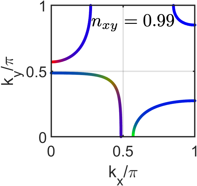
Fig. 1 shows the evolution of the band dispersions as is varied from to 1 while other occupancies are adjusted to maintain the same number of four electrons in the band. We have found that the spin-orbit interaction has a small effect on band renormalizations and therefore, in the following we report the results in the absence of spin-orbit coupling. Fig. 2 shows the evolution of the FS over the same regime. While for sufficiently smaller than the standard Fermi surface topology appears, drastic interaction effects become apparent when .
Indeed, in the coherent regime and thus one expects to have a flat band at , the so-called orbital selective Mott phase (OSMP). In practice, rather than a total localization a finite temperature dependent bandwidth remains that goes to zero as . The fate of this band upon its hybridization with other bands has been debated [63, 67, 68, 69]. We find a finite hybridization that is most manifest in gapping part of the outer hole pocket in Fig. (2). There are significant FS re-constructions in the vicinity of OSMP . In this regime, additional band renormalizations due to Hund’s interaction [70] are expected to be relevant for the OSMP. As the xy orbital is doped further, the hybridization between orbital and grows and the orbital character of the inner FS is strongly modified. In the opposite regime of , the electron pockets and hole pockets are mostly compensated due to the condition we found earlier. At , there is a Lifshitz transition and the system becomes an insulator, in which the finite occupancy of the orbital is supported by the finite admixture in the occupied bands.
There is a window where the xy band is partially occupied, with delocalized excitations. We will focus on this regime and study the pair susceptibility of the model in the next section.
Pair susceptibility: tRVB vs.
As explained in the introduction, experiments on the iron-based superconductors point towards an interplay between orbital selectivity and superconductivity. Motivated by these considerations, here we study the pair susceptibility in this section, providing a comparison between tRVB and states.
In the normal state, the free energy has a Landau-type expansion in . The quadratic term is controlled by the pair susceptibility
| (23) |
where contains the matrix structure of the pairing term. Therefore, determines the onset of pairing. Since we do not have access to the renormalized coupling , we plot the susceptibilities vs. temperature, whose divergence appears as co-centric superconductivity domes. These can be directly compared to the onset of superconductivity in FeSC materials.
The bare pair susceptibility can be written as (Appendix E)
| (24) |
where is the matrix elements of in the band basis
| (25) |
and the matrix acts in orbital/spin/sublattice space. The Pauli principle enforces the relation
| (26) |
Assuming on the FS, the linearly vanishing denominator of (24) leads to a behavior that eventually becomes dominant at low temperature. This is relevant for infinitesimal coupling , but for generic coupling constants, and in particular, large Hund’s coupling, the entire sum in Eq. (24) has significance. For the we choose
| (27) |
where acts in orbital, spin and sublattice spaces but the -factor changes sign at between the electron/hole pockets.
The tRVB state is local and odd in orbital and spin
| (28) |
where the Pauli matrix acts in the sublattice space, playing the role of the staggered part of the tRVB order parameter [9]. In absence of SOI, , where
| (29) |
is the spin-triplet d vector which is odd in parity . It was shown in [9] that is non-zero on the FS, lying in the x-y plane and vanishing at eight notes on the outer hole pocket. A finite SOI, rotates out of the x-y plane and fills the nodes but also adds a singlet admixture to , whose uniform part is similar to the superconducting order parameter proposed by Vafek and Chubukov in Ref. [10]. In addition, there are substantial inter-band and off-resonant contribution to the susceptibility, due to its local nature.


Fig. (3) is the central result of our paper shows a comparison of the pair susceptibility of tRVB and as a function of xy doping and the temperature. The absolute magnitude of the two susceptibilities cannot be compared with each other, due to our lack of knowledge about the coupling constants. However, tRVB is driven by the Hund’s coupling, which assuming a renormalized value of order 0.1eV, predicts a superconducting dome at with a .
V Discussion and Conclusion
Both tRVB and states show a superconducting dome around the doping where electrons in the orbital are delocalized. In the presence of realistic spin-orbit coupling, the mean-field pair susceptibilities of the tRVB state are enhanced by a factor of about five. Moreover, our mean field theory demonstrates a clear correlation between increasing -orbital localization and decreasing for both superconducting states, a feature which is consistent with experimental observations.
Such correlations between occupation and is observed in FeTe1-xSex [71] which exhibits an anti-ferromagnetic (AFM) order at . As is varied [71] from FeTe to FeSe, the antiferromagnetism disappears at about and superconductivity develops at with which depends only weakly on doping in the range . A particularly fascinating feature, is that the renormalization of the band, as determined by the effective mass, diverges as , so that the and bandwidth of the orbital are correlated at low doping, the latter strongly depending on the temperature. It is plausible that as the electrons localize, they produce the AFM order [72].
In summary, we have studied the pair susceptibility of the iron-based superconductors, taking into account the effects of correlations, orbital selectivity and Hund’s interaction. The influence on band renormalization, evolution of orbitals and Fermi surface reconstruction close to the orbital selective Mott transition is captured. Away from the OSMT, a mostly electron-hole compensated Fermi surface develops. We have argued the importance of including charge projectors in the decoupling of the interaction which enable a study of pair susceptibility in terms of physical electrons. Furthermore, this provides a Hund’s driven mechanism for renormalizing down the inter-orbital charge repulsion via spin-fluctuation.
We have performed this calculation for the tRVB state to study the effects of orbital localization and compare it to the s± state. We employed a three-band tight-binding model for this calculation taking into account both intra-band and inter-band contributions to the susceptibility. Both states show a superconducting dome around , but the tRVB state also includes a much weaker superconducting dome close to the orbitally selective Mott phase at due to inter-band contributions.
Acknowledgements.
Acknowledgment - Discussions with S. Fang are appreciated. This work was performed in part at Aspen Center for Physics, which is supported by NSF Grant No. PHY-1607611 and work was also supported by Office of Basic Energy Sciences, Material Sciences and Engineering Division, U.S. Department of Energy (DOE) DE-FG02-99ER45790 (PC and EK).Appendices
The following appendices contain further details and proof of various statements made in the paper.
Appendix A The model
We use the notation
| (30) |
The Hamiltonian is
| (31) |
in terms of [ and denote and .]
| (32) |
and
| (33) |
We also have in terms of . In absence of SOI, it is customary to do a gauge transformation . Then, define uniform and staggered components
| (34) |
and this reduces the problem to [11] with
| (35) |
where
| (36) |
The bare parameters are listed in the table (1).
| 0.06 | 0.02 | 0.03 | -0.01 | 0.2 | 0.3 | -0.2 | 0.4 | 0.212 |
Appendix B Proof of Eq. (4)
The key equation is the Fierz identity
| (37) |
which we rewrite as
| (38) |
We can contract this with and to find
| (39) |
after re-labeling and . Eq. (38) also gives
| (40) |
Subtracting (40) from (39), we obtain
| (41) |
Here, a useful relation is
| (42) |
which expresses the fact that the initial states and final states are either parallel, or antiparallel, coming in with opposite amplitudes. Combining (41) and (42) we find
| (43) | |||||
where we have employed the Fierz equality (38) again in the last step, thus proving Eq. (4). Note that the triplet decoupling (4) is very similar (but has opposite in sign) to the singlet decoupling, which can be obtained from (42) and (43):
| (44) |
Appendix C Five-band to three-band reduction
FeSCs are usually described by three-band [64] or five-band [73, 74] models. This extensively discussed in [7, 75]. Since the orbitals mix with orbitals, Fig. 4(a,b), it cannot be ignored and since according to DFT calculations it crosses the chemical potential, it’s effect is beyond a merely renormalization of the tight-binding parameters. However, as we show here, an effective 3-band model provides a faithful representation of the material close to the Fermi energy. The Green’s function for the 5-band system is
| (45) |
where
| (46) |
Focusing on orbitals, the Green’s function is
| (47) |
where
| (48) |
which motivates defining the static Hamiltonian [76]
| (49) |
Fig. 4(c,d) shows the band structure and FS of . Clearly, the spectrum diverges at points in the BZ and therefore, a tight-binding representation is not available. However, the FS is captured faithfully and this effective Hamiltonian can use it for practical calculation.

Note that appears as an infinity of or a zero of the effective Green’s function. Here, we will discuss the occupancy of the effective Hamiltonian, showing that the orbital will have an occupancy that includes the zeros of the Green’s function due to integrated-out states. According to the Luttinger’s theorem
| (50) |
where is the dimensionality and the FS volume is
| (51) |
so that any place where is counted as occupied state. Denoting , with , and there are two ways the Green’s function can change sign: through poles , covering the total area in the BZ, or through zeros , covering the area . This leads to the following relation:
| (52) |
Therefore, poles alone enclose an enlarged area that contains the FS of the integrated-over orbitals. In the present case, bands have occupancy 2. Therefore, the effective orbital has the occupancy of 4.
Appendix D Hund’s driven attraction, beta function
In this section, we should that the decoupled Hund’s coupling in the normal state of the tRVB order parameter creates an attractive interaction between the orbitals. For simplicity, we consider an infinite- impurity setting, where a single Fe atom is hybridized with conduction electrons, which realizes a DMFT setting. For simplicity, we assume
We assume each orbital has its own bath, with a hybridization that can depend on energy. The Hamiltonian is where contains the conduction electron and their hybridization with different orbitals of Fe. The interaction is given by
| (53) | |||||
Here we have introduced super-index and where are orbital and are spin degrees of freedom and it is understood that . contains Lagrange multipliers that impose the infinite intra-orbital constraint. For simplicity we have assumed the occupancy of all the orbitals is less than one. This could easily changed by doing and with the notation of the paper.


We would like to do an RG studies of this Hamiltonian. We can write the partition function in the interaction picture w.r.t. :
| (54) |
and compute to second order in , representing and . This is shown by the Feynman diagram 5(b). We use the fact that within the time-scale beside a phase evolution by , the holons are slowly varying so that
| (55) |
For the second order term we find
At this point we make some simplifying assumption. First we assume that interaction effects can be neglected and we are in the normal phase. This means we can apply the Wick’s contraction
| (56) | |||
Next, we assume we are in the paramagnetic regime and different orbitals are not correlated at high-temperature, meaning that fermion propagators are diagonal in spin and orbital, although orbital asymmetry can be present. The two terms in Eq. (56) add up:
where denote the orbital index of subindices and we have used Eq. (26) to deduce . For the tRVB state ,
| (57) |
Moreover, in the normal phase the propagator is approximately constant and equal to the inverse (renormalized) coupling constant
| (58) |
Then we can write
| (59) | |||||
At high energies can be dropped out with a similar term with an opposite sign inside . We have assumed each orbital is in the Fermi liquid state with a bandwidth governed by . Therefore, doing the integral and replacing we find
| (60) |
This has the same form as the term and can be absorbed to renormalize its value
| (61) |
or using and defining , the dimensionless coupling is modified to
| (62) |
We add to this a tree-level renormalization of the relevant operator which arises due to scaling of .
which means
| (64) |
So, adding these two contributions we find
| (65) |
Appendix E Pair susceptibility
We consider a pairing terms of the type
| (66) |
where are super-indices containing orbital/spin/sublattice and denotes the relative position of the two electrons in a Cooper pair. Note that the order parameter has the symmetry
| (67) |
due to Pauli principle. A second-order perturbation theory in gives a contribution to the Free energy where the susceptibility is given by
| (68) | |||||
expressed in terms of the fermionic bubble
| (69) |
Bare Susceptibility
Using Wick’s contraction we find
The Green’s functions can be expressed as
| (70) |
in terms of . Doing the imaginary-time integral, and the Matsubara sum and using that the two terms in Eq. (68) are equal we find
Finally, using the anti-symmetry of the order parameter (67) and that the spectral function in the band-basis has a simple form
| (71) |
Susceptibility from mean-field theory
In this case
| (72) |
where
| (73) | |||
| (74) |
We can apply Wick’s contraction to each of these four-point functions and using Eq. (70) find
Using Eq. (71) we find
A numerical evaluation of this sum is computationally costly. A simplification happens in the coherent regime which happens for one of the bosonic bands. In that case, and we find the same equation as Eq. (24) except that the renormalized is given by
| (76) |
We examine this approximation closely in the single-band Hubbard model.
Appendix F Single-band Hubbard model
In the limit of infinite-, the single-band Hubbard is mapped to the model,
| (77) | |||||
The -term can be decoupled in the singlet channel using Eq. (44) in particle-hole and particle-particle channels. Again, both channels are attractive and can acquire finite expectation value. We find
| (78) | |||||
The new feature compared to [62] is the additional factor of which result from decoupling of hidden charge projectors in (77). The two channels and behave differently as is being driven by the and just renormalizes . So, we can write where
| (79) |
Note that this Hamiltonian is expressed entirely in terms of infinite- real electrons . The plan we follow in this paper is to solve this problem in the normal state using mean-field decoupling of holons and fermions and then compute the pair susceptibility of the real electrons. A mean-field decoupling gives up to a constant shift in energy
| (80) |
where
| (81) |
At low-T, we find whereas is determined by the average kinetic energy of occupied fermions. A self-consistent solution to these equations represent a fixed point solution (in a statistical mechanical sense) to the interacting problem . In terms of these . Using translational invariance
| (82) |
At low temperature and sufficiently large dimension, the bosons will condense. The computation below is done in a finite system size and contains this transition as a crossover. A comment about possible interaction
| (83) |
is in order. Clearly can derive various forms of charge-density wave. Within the mean-field theory and as long as translational invariance is assumed, this interaction does not play any role and only changes the relation between chemical potential and the doping. Next, we compute the pair susceptibility for this state, assuming translational invariance . For the d-wave,
| (84) |
It is convenient to define a form-factor
| (85) |
The pair susceptibility is
expressed in terms of the fermion/holon bubbles,
| (86) |
A straightforward calculation gives a simplified version of the expression from the previous appendix:
| (87) |
where
| (88) | |||||
. At low-T, we can approximate . The first term gives the usual contribution
| (89) |
These two functions are shown side-by-side in Fig…
A problem is that both over-estimate the value of the optical doping. We suspect that this is due to the mean-field decoupling.


Appendix G Slave-boson mean-field calculation
Diagonalizing Bosonic Hamiltonian
Since we have used mixed holon-doublon description of the orbitals, the bosonic Hamiltonian will contain bosonic pairing terms. For an -orbital problem we form the Hamiltonian
| (90) |
Rotating to form we obtain
| (91) |
The Hamiltonian becomes
| (92) |
where is real, symmetric and positive definite and can be diagonalized [77] using a symplectic transformation .
| (93) |
where is a diagonal matrix containing symplectic eigenvalues. Therefore, the original bosons are related via to a new set of canonical boson
| (94) |
in terms of which the Hamiltonian is diagonal:
| (95) |
Details of the procedure
After a decoupling, we find
| (96) |
in terms of bosonic and fermionic operators
| (97) |
We assume that spinons inherit the symmetry of the electron orbitals, whereas bosons are invariant under crystal rotations. Therefore, has the same form as only with renormalized parameters. is similar, with the difference that all are replaced with .
References
- Hosono et al. [2018] H. Hosono, A. Yamamoto, H. Hiramatsu, and Y. Ma, Recent advances in iron-based superconductors toward applications, Materials Today 21, 278 (2018).
- Mazin et al. [2008] I. I. Mazin, D. J. Singh, M. D. Johannes, and M. H. Du, Unconventional Superconductivity with a Sign Reversal in the Order Parameter of , Phys. Rev. Lett. 101, 057003 (2008).
- Hirschfeld et al. [2011] P. J. Hirschfeld, M. M. Korshunov, and I. I. Mazin, Gap symmetry and structure of fe-based superconductors, Reports on Progress in Physics 74, 124508 (2011).
- Chubukov [2012] A. Chubukov, Pairing mechanism in fe-based superconductors, Annual Review of Condensed Matter Physics 3, 57 (2012).
- Chubukov [2015] A. V. Chubukov, Itinerant electron scenario for Fe-based superconductors 10.48550/arxiv.1507.03856 (2015).
- Si and Abrahams [2008] Q. Si and E. Abrahams, Strong correlations and magnetic frustration in the high iron pnictides, Phys. Rev. Lett. 101, 076401 (2008).
- Fernandes and Chubukov [2016] R. M. Fernandes and A. V. Chubukov, Low-energy microscopic models for iron-based superconductors: a review, Reports on Progress in Physics 80, 014503 (2016).
- Xu et al. [2020] Z. Xu, G. Dai, Y. Li, Z. Yin, Y. Rong, L. Tian, P. Liu, H. Wang, L. Xing, Y. Wei, R. Kajimoto, K. Ikeuchi, D. L. Abernathy, X. Wang, C. Jin, X. Lu, G. Tan, and P. Dai, Strong local moment antiferromagnetic spin fluctuations in v-doped LiFeAs, npj Quantum Materials 5, 10.1038/s41535-020-0212-x (2020).
- Coleman et al. [2020] P. Coleman, Y. Komijani, and E. J. König, Triplet resonating valence bond state and superconductivity in hund’s metals, Phys. Rev. Lett. 125, 077001 (2020).
- Vafek and Chubukov [2017] O. Vafek and A. V. Chubukov, Hund interaction, spin-orbit coupling, and the mechanism of superconductivity in strongly hole-doped iron pnictides, Phys. Rev. Lett. 118, 087003 (2017).
- Lee and Wen [2008] P. A. Lee and X.-G. Wen, Spin-triplet -wave pairing in a three-orbital model for iron pnictide superconductors, Phys. Rev. B 78, 144517 (2008).
- Puetter and Kee [2012] C. M. Puetter and H.-Y. Kee, Identifying spin-triplet pairing in spin-orbit coupled multi-band superconductors, EPL (Europhysics Letters) 98, 27010 (2012).
- Hu [2013] J. Hu, Iron-based superconductors as odd-parity superconductors, Phys. Rev. X 3, 031004 (2013).
- Hao and Hu [2014a] N. Hao and J. Hu, Odd parity pairing and nodeless antiphase in iron-based superconductors, Phys. Rev. B 89, 045144 (2014a).
- Hao and Hu [2014b] N. Hao and J. Hu, Topological phases in the single-layer fese, Phys. Rev. X 4, 031053 (2014b).
- Georges et al. [1996] A. Georges, G. Kotliar, W. Krauth, and M. J. Rozenberg, Dynamical mean-field theory of strongly correlated fermion systems and the limit of infinite dimensions, Rev. Mod. Phys. 68, 13 (1996).
- Haule et al. [2008] K. Haule, J. H. Shim, and G. Kotliar, Correlated electronic structure of , Phys. Rev. Lett. 100, 226402 (2008).
- Haule and Kotliar [2009] K. Haule and G. Kotliar, Coherence-incoherence crossover in the normal state of iron oxypnictides and importance of hund’s rule coupling, New Journal of Physics 11, 025021 (2009).
- Yin et al. [2011] Z. P. Yin, K. Haule, and G. Kotliar, Kinetic frustration and the nature of the magnetic and paramagnetic states in iron pnictides and iron chalcogenides, Nature Materials 10, 932 (2011).
- Yin et al. [2012] Z. P. Yin, K. Haule, and G. Kotliar, Fractional power-law behavior and its origin in iron-chalcogenide and ruthenate superconductors: Insights from first-principles calculations, Phys. Rev. B 86, 195141 (2012).
- Georges et al. [2013] A. Georges, L. d. Medici, and J. Mravlje, Strong correlations from hund’s coupling, Annu. Rev. Condens. Matter Phys. 4, 137 (2013).
- Deng et al. [2019] X. Deng, K. M. Stadler, K. Haule, A. Weichselbaum, J. von Delft, and G. Kotliar, Signatures of mottness and hundness in archetypal correlated metals, Nature Communications 10, 10.1038/s41467-019-10257-2 (2019).
- Schrieffer [1967] J. R. Schrieffer, The kondo effect—the link between magnetic and nonmagnetic impurities in metals?, Journal of Applied Physics 38, 1143 (1967).
- Nevidomskyy and Coleman [2009] A. H. Nevidomskyy and P. Coleman, Kondo resonance narrowing in-and -electron systems, Physical Review Letters 103, 147205 (2009).
- Stadler et al. [2015] K. M. Stadler, Z. P. Yin, J. von Delft, G. Kotliar, and A. Weichselbaum, Dynamical mean-field theory plus numerical renormalization-group study of spin-orbital separation in a three-band hund metal, Phys. Rev. Lett. 115, 136401 (2015).
- Drouin-Touchette et al. [2021] V. Drouin-Touchette, E. J. König, Y. Komijani, and P. Coleman, Emergent moments in a hund’s impurity, Physical Review B 103, 205147 (2021).
- Werner et al. [2008] P. Werner, E. Gull, M. Troyer, and A. J. Millis, Spin freezing transition and non-fermi-liquid self-energy in a three-orbital model, Physical Review Letters 101, 166405 (2008).
- Hoshino and Werner [2015] S. Hoshino and P. Werner, Superconductivity from emerging magnetic moments, Phys. Rev. Lett. 115, 247001 (2015).
- Miao et al. [2018] H. Miao, W. Brito, Z. Yin, et al., Universal scaling decoupled from the electronic coherence in iron-based superconductors, Physical Review B 98, 020502(R) (2018).
- Lee et al. [2018] T.-H. Lee, A. Chubukov, H. Miao, and G. Kotliar, Pairing mechanism in Hund’s metal superconductors and the universality of the superconducting gap to critical temperature ratio, Phys. Rev. Lett. 121, 187003 (2018).
- Classen and Chubukov [2021] L. Classen and A. Chubukov, Superconductivity of incoherent electrons in the yukawa sachdev-ye-kitaev model, Phys. Rev. B 104, 125120 (2021).
- Inkof et al. [2022] G.-A. Inkof, K. Schlam, and J. Schmalian, npj quantum materials 7, 56 (2022).
- Wal [2020] Uncovering non-fermi-liquid behavior in hund metals: Conformal field theory analysis of an spin-orbital kondo model, Physical Review X 10, 031052 (2020).
- Drouin-Touchette et al. [2022] V. Drouin-Touchette, E. J. König, Y. Komijani, and P. Coleman, Interplay of charge and spin fluctuations in a hund’s coupled impurity (2022).
- de’ Medici et al. [2014] L. de’ Medici, G. Giovannetti, and M. Capone, Selective mott physics as a key to iron superconductors, Phys. Rev. Lett. 112, 177001 (2014).
- Sprau et al. [2017] P. O. Sprau, A. Kostin, A. Kreisel, A. E. Böhmer, V. Taufour, P. C. Canfield, S. Mukherjee, P. J. Hirschfeld, B. M. Andersen, and J. C. S. Davis, Discovery of orbital-selective Cooper pairing in FeSe, Science 357, 75 (2017).
- Klug et al. [2018] M. Klug, J. Kang, R. M. Fernandes, and J. Schmalian, Orbital loop currents in iron-based superconductors, Physical Review B 97, 155130 (2018).
- Yue and Werner [2021] C. Yue and P. Werner, Pairing enhanced by local orbital fluctuations in a model for monolayer FeSe, Physical Review B 104, 184507 (2021).
- Yi et al. [2013] M. Yi, D. H. Lu, R. Yu, S. C. Riggs, J.-H. Chu, B. Lv, Z. K. Liu, M. Lu, Y.-T. Cui, M. Hashimoto, S.-K. Mo, Z. Hussain, C. W. Chu, I. R. Fisher, Q. Si, and Z.-X. Shen, Observation of temperature-induced crossover to an orbital-selective mott phase in (, rb) superconductors, Phys. Rev. Lett. 110, 067003 (2013).
- Yi et al. [2017] M. Yi, Y. Zhang, Z.-X. Shen, and D. Lu, Role of the orbital degree of freedom in iron-based superconductors, npj Quantum Materials 2, 10.1038/s41535-017-0059-y (2017).
- Bogolyubov et al. [1958] N. Bogolyubov, V. Tolmachev, and D. Shirkov, Noviy metod v teorii sverkhprovodimosti (Izdatel’stvo akademii nauk SSSR, Moscow, 1958) [Engl. transl. ”A new method in the theory of superconductivity”, Consultants Bureau, New York, 1959.].
- McMillan [1968] W. L. McMillan, Transition temperature of strong-coupled superconductors, Phys. Rev. 167, 331 (1968).
- Anderson and Morel [1961] P. W. Anderson and P. Morel, Generalized bardeen-cooper-schrieffer states and the proposed low-temperature phase of liquid , Phys. Rev. 123, 1911 (1961).
- Coleman [2015] P. Coleman, Introduction to Many-Body Physics (Cambridge University Press, 2015).
- König and Coleman [2019] E. J. König and P. Coleman, Coulomb problem in iron-based superconductors, Phys. Rev. B 99, 144522 (2019).
- Anderson [1987] P. W. Anderson, Science 235, 1196 (1987).
- Anderson et al. [1987] P. W. Anderson, G. Baskaran, Z. Zou, and T. Hsu, Resonating-valence-bond theory of phase transitions and superconductivity in la2cuo4-based compounds, Physical Review Letters 58, 2790 (1987).
- Baskaran et al. [1987] G. Baskaran, Z. Zou, and P. Anderson, The resonating valence bond state and high-tc superconductivity — a mean field theory, Solid State Communications 63, 973 (1987).
- Lee et al. [2006] P. A. Lee, N. Nagaosa, and X.-G. Wen, Doping a Mott insulator: Physics of high-temperature superconductivity, Rev. Mod. Phys. 78, 17 (2006).
- Anderson [1984a] P. W. Anderson, Heavy-electron superconductors, spin fluctuations, and triplet pairing, Phys. Rev. B 30, 1549 (1984a).
- Anderson [1984b] P. W. Anderson, Structure of ”triplet” superconducting energy gaps, Phys. Rev. B 30, 4000 (1984b).
- Anderson [1985] P. W. Anderson, Further consequences of symmetry in heavy-electron superconductors, Phys. Rev. B 32, 499 (1985).
- Shen et al. [2020] B. Shen, Y. Zhang, Y. Komijani, M. Nicklas, R. Borth, A. Wang, Y. Chen, Z. Nie, R. Li, X. Lu, et al., Strange-metal behaviour in a pure ferromagnetic kondo lattice, Nature 579, 51 (2020).
- König et al. [2022] E. J. König, Y. Komijani, and P. Coleman, Triplet resonating valence bond theory and transition metal chalcogenides, Physical Review B 105, 075142 (2022).
- Lopez et al. [2022] M. Lopez, B. Powell, and J. Merino, Topological superconductivity from doping a triplet quantum spin liquid in a flat band system, (2022), arXiv:2210.05275 .
- Carretta and Prando [2020] P. Carretta and G. Prando, Iron-based superconductors: tales from the nuclei, La Rivista del Nuovo Cimento 43, 1 (2020).
- Hanaguri et al. [2010] T. Hanaguri, S. Niitaka, K. Kuroki, and H. Takagi, Unconventional s-wave superconductivity in Fe (Se, Te), Science 328, 474 (2010).
- Chi et al. [2014] S. Chi, S. Johnston, G. Levy, S. Grothe, R. Szedlak, B. Ludbrook, R. Liang, P. Dosanjh, S. A. Burke, A. Damascelli, D. A. Bonn, W. N. Hardy, and Y. Pennec, Sign inversion in the superconducting order parameter of LiFeAs inferred from bogoliubov quasiparticle interference, Phys. Rev. B 89, 104522 (2014).
- Barnes [1976] S. E. Barnes, New method for the anderson model, Journal of Physics F: Metal Physics 6, 1375 (1976).
- Coleman [1984] P. Coleman, New approach to the mixed-valence problem, Physical Review B 29, 3035 (1984).
- Ruckenstein et al. [1987] A. E. Ruckenstein, P. J. Hirschfeld, and J. Appel, Mean-field theory of high- superconductivity: The superexchange mechanism, Phys. Rev. B 36, 857 (1987).
- Kotliar and Liu [1988] G. Kotliar and J. Liu, Superexchange mechanism and d-wave superconductivity, Phys. Rev. B 38, 5142 (1988).
- Yu and Si [2013] R. Yu and Q. Si, Orbital-selective mott phase in multiorbital models for alkaline iron selenides , Phys. Rev. Lett. 110, 146402 (2013).
- Daghofer et al. [2010] M. Daghofer, A. Nicholson, A. Moreo, and E. Dagotto, Three orbital model for the iron-based superconductors, Phys. Rev. B 81, 014511 (2010).
- Albuquerque et al. [2012] A. F. Albuquerque, F. Alet, and R. Moessner, Coexistence of long-range and algebraic correlations for short-range valence-bond wave functions in three dimensions, Phys. Rev. Lett. 109, 147204 (2012).
- Eschrig and Koepernik [2009a] H. Eschrig and K. Koepernik, Tight-binding models for the iron-based superconductors, Phys. Rev. B 80, 104503 (2009a).
- Yu and Si [2017] R. Yu and Q. Si, Orbital-selective mott phase in multiorbital models for iron pnictides and chalcogenides, Phys. Rev. B 96, 125110 (2017).
- Komijani and Kotliar [2017] Y. Komijani and G. Kotliar, Analytical slave-spin mean-field approach to orbital selective mott insulators, Phys. Rev. B 96, 125111 (2017).
- Komijani et al. [2019] Y. Komijani, K. Hallberg, and G. Kotliar, Renormalized dispersing multiplets in the spectrum of nearly mott localized systems, Physical Review B 99, 125150 (2019).
- Si et al. [2016] Q. Si, R. Yu, and E. Abrahams, High-temperature superconductivity in iron pnictides and chalcogenides, Nature Reviews Materials 1, 16017 (2016).
- Liu et al. [2015] Z. K. Liu, M. Yi, Y. Zhang, J. Hu, R. Yu, J.-X. Zhu, R.-H. He, Y. L. Chen, M. Hashimoto, R. G. Moore, S.-K. Mo, Z. Hussain, Q. Si, Z. Q. Mao, D. H. Lu, and Z.-X. Shen, Experimental observation of incoherent-coherent crossover and orbital-dependent band renormalization in iron chalcogenide superconductors, Phys. Rev. B 92, 235138 (2015).
- Huang et al. [2022] J. Huang, R. Yu, Z. Xu, J.-X. Zhu, J. S. Oh, Q. Jiang, M. Wang, H. Wu, T. Chen, J. D. Denlinger, S.-K. Mo, M. Hashimoto, M. Michiardi, T. M. Pedersen, S. Gorovikov, S. Zhdanovich, A. Damascelli, G. Gu, P. Dai, J.-H. Chu, D. Lu, Q. Si, R. J. Birgeneau, and M. Yi, Correlation-driven electronic reconstruction in FeTe1-xSex, Communications Physics 5, 10.1038/s42005-022-00805-6 (2022).
- Graser et al. [2009] S. Graser, T. A. Maier, P. J. Hirschfeld, and D. J. Scalapino, Near-degeneracy of several pairing channels in multiorbital models for the fe pnictides, New Journal of Physics 11, 025016 (2009).
- Eschrig and Koepernik [2009b] H. Eschrig and K. Koepernik, Tight-binding models for the iron-based superconductors, Phys. Rev. B 80, 104503 (2009b).
- Borisenko et al. [2016] S. Borisenko, D. Evtushinsky, Z.-H. Liu, I. Morozov, R. Kappenberger, S. Wurmehl, B. Büchner, A. Yaresko, T. Kim, M. Hoesch, et al., Direct observation of spin–orbit coupling in iron-based superconductors, Nature Physics 12, 311 (2016).
- Wang and Zhang [2012] Z. Wang and S.-C. Zhang, Simplified topological invariants for interacting insulators, Physical Review X 2, 031008 (2012).
- Son et al. [2021] N. T. Son, P.-A. Absil, B. Gao, and T. Stykel, Computing symplectic eigenpairs of symmetric positive-definite matrices via trace minimization and riemannian optimization, SIAM Journal on Matrix Analysis and Applications 42, 1732 (2021).