Triple-meron crystal in high-spin Kitaev magnets

Introduction. – Topological spin textures (TSTs), which have attracted enormous attention in condensed matter physics, can be described by the homotopy theoryBraun2012 with a non-trivial mapping $\pi_{n}(S^{m})$, where $n$ and $m$ are the corresponding degrees of freedom in the real and the parameter spaces, respectively. A topological charge $Q$ thus counts the number of times of the real space configuration covering the parameter space. Among these TSTs, the skyrmions ($\pi_{2}(S^{2})$), originally proposed in the particle physicsSkyrme1962 , have become the focus of recent research in magnetism due to their potential applications in spintronicsNagaosaTokura2013 ; FertRC2017 ; HellmanHTetal2017 ; Zhou2018 ; BogdanovPanagopoulos2020 ; GobelMT2021 . Experimentally, they have already been successfully discovered in noncentrosymmetric chiral magnets MuhlbauerBJetal2009 ; YuOKetal2010 ; SekiYIT2012 ; NayakKMetal2017 ; FujishiroKNetal2019 , magnetic heterostructures HeinzeBMetal2011 ; RommingHMetal2013 ; TokunagaYRetal2015 ; MoreauMRetal2016 and centrosymmetric magnets KurumajiNHetal2019 ; HirschbergerNGetal2019 ; KhanhNYetal2020 . In a skyrmion, $Q$ is an integer which is given byBraun2012

where ${\bf{S}=\bf{S}}(x,y)$ is the unit spin vector at the position $(x,y)$. In addition, recent studies show that, given a sufficiently large effective easy-plane anisotropy, a skyrmion can be transferred into a meron-antimeron pairLinSB2015 ; YuKTetal2018 ; GaoJIetal2019 ; GaoRGetal2020 . Such meron and antimeron carry one half skyrmion topological charge, and thus are treated as half skyrmions. From the spin configurations, the most distinct difference between skyrmions and merons is that at the perimeter the spins of merons lie within the plane while those of skyrmions point out of the plane.

On the other hand, ever since the discovery of the exact solution of the Kitaev honeycomb modelKitaev2006 , great efforts have been made to synthesize materials to realize such a model. These materials, so called Kitaev magnets, are two-dimensional transition-metal compounds with strong spin-orbit coupling JackeliKhaliullin2009 . The promising candidates include $\rm Na_{2}IrO_{3}$, $\rm Li_{2}IrO_{3}$ and $\rm\alpha$-$\rm RuCl_{3}$ SinghMRetal2012 ; PlumbCSetal2014 . In these compounds, honeycomb-located cations are surrounded by the edge-sharing octahedral anions. Strong spin-orbit coupling entangles spin and orbital degrees of freedom together, resulting in an effective spin-1/2 model with the Heisenberg ($J$) and Kitaev ($KS_{i}^{\gamma}S_{j}^{\gamma}$) interactions. Further research suggests that a bond-dependent symmetric off-diagonal $\Gamma$ and/or $\Gamma^{\prime}$ interactions should also be taken into accountRauLK2014 ; KatukuriNYetal2014 ; WangDYetal2017 . This $\rm{JK\Gamma\Gamma^{\prime}}$ model and its relevance have been proposedMaksimovChernyshev2020 to explain the possible quantum spin liquids observed in experiments.

However, the Kitaev interaction is not limited to spin-1/2 compounds. Recent numerical and theoretical analysisXuFXetal2018 ; LeeUWetal2020 ; StavropoulosPLetal2021 suggest that it may also exist in the van der Waals materials $\rm CrI_{3}$, $\rm CrGeTe_{3}$ and $\rm CrSiTe_{3}$. Interestingly, the crystal structures of these compounds bear a strong resemblance to those of the honeycomb iridates but Cr owns an effective $S=3/2$ spin. Similar to its spin-1/2 counterparts these compounds can also be described by the $\rm JK\Gamma\Gamma^{\prime}$ model but possibly with an additional single-ion anisotropy ($A$). Although the sought-after quantum spin liquids are not preferable in these high-spin Kitaev magnetsZhouCLetal2021 , stable TSTs originating from frustration OkuboCK2012 ; LeonovMostovoy2015 ; HayamiOM2017 ; KharkovSM2017 ; WangSLetal2021 are highly desirable. This calls for extensive and immediate studies to search for the TSTs in these high-spin Kitaev magnets. However, so far, most works focus simply on the magnetic ordersChernKLetal2020 ; LiuSRetal2020 ; RayyanLK2021 but relevant topological phenomena are rarely touched. We fill in this gap by investigating the classical $\rm K\Gamma{A}$ model numerically. A triple-meron crystal (TmX) with three (anti)merons in one magnetic unit cell (MUC) is discovered, suggesting the mechanism for generating (anti)merons is beyond our present knowledge. Furthermore, we show that such a TmX can cause the topological Hall effect (THE)Hamamoto2015 which is absent in the meron-antimeron crystalsHayamiOM2021 .

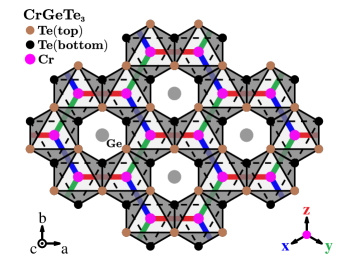
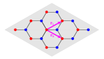
Model. – The crystal structuresHuangCNetal2017 ; GongLLetal2017 ; XingCOetal2017 ; XuFXetal2018 of the Cr-based compounds mentioned above are sketched in Fig. 1. Due to their similarity, here we exemplify them by the $\rm{CrGeTe_{3}}$. In $\rm{CrGeTe_{3}}$ six Te atoms are at the corners of an octahedron and the Cr atom sits at the center. These edge-shared octahedrons form honeycomb layers stacking along the c axis, which are stabilized by a weak interlayer van der Waals coupling. Due to the symmetry of the crystal, two coordinate systemsXuFXetal2018 , $\rm\bf{abc}$ and $\rm\bf{xyz}$ are involved in our later discussion (Fig. 1). In principle, $J,K,\Gamma,\Gamma^{\prime}$ and $A$ terms are all allowed by the lattice symmetry. However, for a given compound, some terms may be zero. For example, the density-functional theory calculation shows that in $\rm CrGeTe_{3}$ the Heisenberg term $J$ becomes zero at some compressive strainXuFKetal2020 . Here, for simplicity, we consider the $\rm K\Gamma A$ model, which is given by

where $\langle{i,j}\rangle$ means that the summation runs over all nearest neighbors. $S_{i}^{\gamma}=\mathbf{S}_{i}\cdot\vec{\gamma}(\vec{\gamma}=\bf{x,y,z})$, e.g., the $\gamma$-component of the spin vector at site $i$ associated with the $\gamma$ bonds on the honeycomb lattice and $\alpha,\beta$ are other two components. This Hamiltonian can be parameterized as $K=\textrm{sin}\theta\cos\phi$, $\Gamma=\sin\theta\sin\phi$ and $A=\cos\theta$, with $\mathbf{\theta}\in[0,\pi]$ and $\mathbf{\phi}\in[0,2\pi)$. Now the model (2) depends on only two parameters $\theta$ and $\phi$. Furthermore, one can see that the transformation $\mathbf{\phi}\rightarrow\mathbf{\phi+\pi}$ is equivalent to flipping all the spins in one sublattice. Therefore, we only need to consider the parameters in the region $\phi\in[0,\pi)$.

To get the ground-state phase diagram, the Hamiltonian (2) is studied by the parallel-tempering Monte Carlo simulationsHukushimaNemoto1996 ; MetropolisRRetal1953 ; MiyatakeYKetal1986 ; JanssenAV2016 in combination with other numerical techniques (Supplementary Material (SM)Supp Sec. I). In our Monte Carlo simulations, the maximum size is $2\times 36\times 36$ and the temperature ranges from 0.005 to 0.2. The ground state is then obtained by optimizing the Monte Carlo data. Various sizes are used to confirm we obtain the correct MUC (SMSupp Sec. II). The ground-state energy, the spin configurations and the static spin structure factor are calculated to map out the phase diagram. In the following, all the figures are plotted in the abc coordinate system.

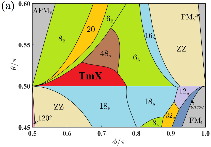
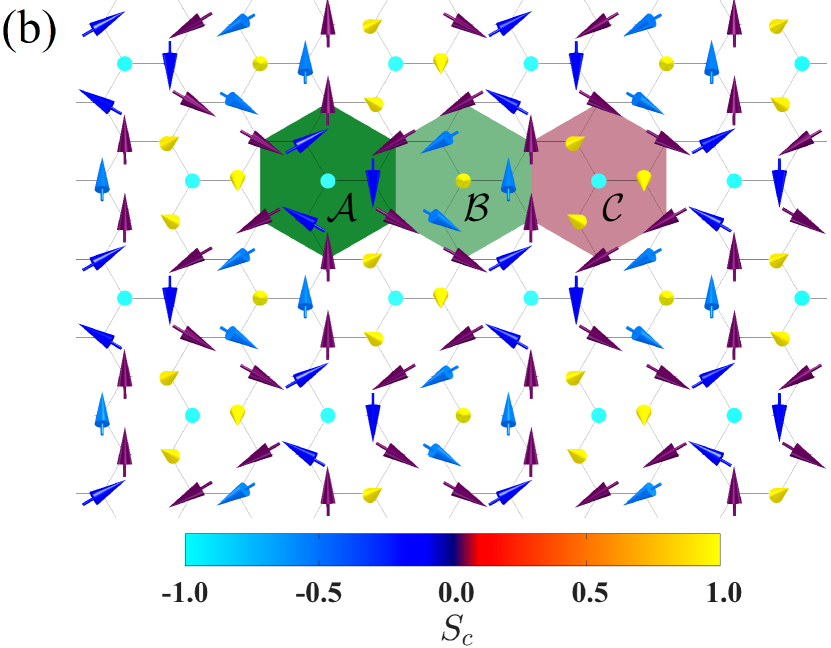
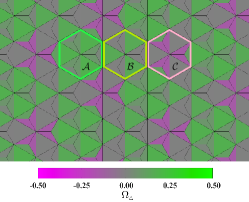
Results. – In Fig. 2(a), we present the ground-state phase diagram of the $\rm K\Gamma{A}$ model in the region $\theta\in[0.45\pi,0.60\pi]$, $\phi\in[0.5\pi,1.0\pi]$ (see SMSupp Sec. VI for the full phase diagram). Of all these phases, the one in red marked by $\rm{TmX}$ is the most exciting discovery in our work. In the following, we will focus on this phase and present the details. For simplicity, we choose one representative point in the TmX phase, i.e., $\theta=0.515\pi,\phi=0.68\pi$ to demonstrate its unusual properties. In Fig. 2(b), we plot the ground-state spin configuration at the representative point. One can see there are 18 spins in one MUC. Moreover, these 18 spins are divided into three hexagons with their edges shared, which are marked by $\mathcal{A}$, $\mathcal{B}$ and $\mathcal{C}$, respectively. After a simple inspection one finds the spin at the core of each hexagon points out of the plane, while the edge spins lie almost in the plane. This is the characteristic feature of (anti)merons, indicating that there are three (anti)merons in one MUC. This finding is very distinct from our previous knowledge that the meron and antimeron should emerge in pairsLinSB2015 ; YuKTetal2018 ; GaoJIetal2019 ; GaoRGetal2020 . In a common sense, the meron and antimeron with a topological charge $\mp{1/2}$ can be mappedLinSB2015 onto the southern and northern hemispheres, respectively, and wrap them once. Hence, considering a large enough easy-plane interaction, such as an in-plane anisotropy or the dipole-dipole interaction, a skyrmion could be dissociated into two halves from the equator, transforming into a meron-antimeron pairLinSB2015 . However, as shown in Fig. 2(b), there are three Bloch-type (anti)merons. Each one is composed of ten spins, including one polarized core spin, its three nearest neighbours (NNs) and six next-nearest neighbours (NNNs). All the core spins locate on the same sublattice, and are completely polarized along the $\rm\mathbf{c}$ axis (down for $\mathcal{A}$ and $\mathcal{C}$, up for $\mathcal{B}$). The three NNs of each (anti)meron locate on the other sublattice and have the same polar angle. In particular, in $\mathcal{B}$ and $\mathcal{C}$ they are on the opposite hemisphere to the core spin. At the edges, the equator is formed by six NNNs locating on the same sublattice as the core spin. All NNNs lie almost in the $\mathbf{ab}$ plane. These characters suggest that $\mathcal{B}$ and $\mathcal{C}$ are of the AFM type. We want to mention that in our model FM merons are readily available by the transformation $\phi\rightarrow\phi+\pi$, equivalent to flipping all spins on one sublattice.

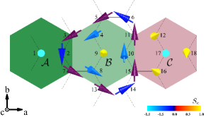
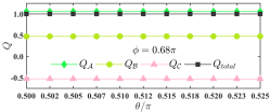
One could notice that, if swirling around one meron in any direction, its NN and NNN spins rotate in the same direction while the core spins in $\mathcal{B}$ and $\mathcal{C}$ are antiparallel. In addition, for one loop around the meron, the spins in $\mathcal{A}$ rotate $4\pi$, wrapping the hemisphere twice. By contrast, the spins wrap the hemisphere once in $\mathcal{B}$ and $\mathcal{C}$, suggesting the topological charge of $\mathcal{A}$ should be twice of those of $\mathcal{B}$ and $\mathcal{C}$. In order to confirm our analysis, we calculate the topological charges of the three merons at the representative parameter point following the definition given by Berg and LüscherBergLuscher1981  (SMSupp Sec. III), which turn out to be $Q_{\mathcal{A}}=1.055231,Q_{\mathcal{B}}=0.472850$ and $Q_{\mathcal{C}}=-0.528081$, indicating the existence of a meron ($Q_{\mathcal{C}}$) and antimeron ($Q_{\mathcal{B}}$) pair and a high-$Q$ antimeron ($Q_{\mathcal{A}}$). Particularly, the high-$Q$ antimeron is topologically equivalent to a half high-$Q$ antiskyrmionZhangZhouEzawa2016 . It is known theoretically that the topological charge for a ideal (high-$Q$) (anti)meron should be exactly $n/2$ with $n$ an integer. However, in the lattice system, the three (anti)merons share the outmost spins as the equator. When frustrations disturb the outmost edge slightly off the $\mathbf{ab}$ plane, we can expect that the topological charge of each (anti)meron may deviate from its theoretical value accordingly. Since the increase or decrease of solid angles should occur synchronously and one can expect that the summation of $Q_{\mathcal{A}},Q_{\mathcal{B}}$ and $Q_{\mathcal{C}}$ should be an integer. Indeed, this is what we have observed from our results, i.e., it is 1.0. Particularly, in the TmX phase there are points with their $Q_{\mathcal{A}},Q_{\mathcal{B}}$ and $Q_{\mathcal{C}}$ agreeing well with their theoretical values and the summation giving 1.0 as well.

The crystals formed by magnetic spin textures with a nonzero $Q$ often exhibit nontrivial transport properties. The prototypical example is the THEHamamoto2015 . However, it has been shown HayamiOM2021 that there is no THE in the meron-antimeron crystals due to the vanishing net $Q$. Thus, the TmX provides an opportunity to explore the THE in the meron crystals. To show this, we study the double-exchange model, which describes itinerant electrons coupled with the spin textureHamamoto2015 ,

where $c^{\dagger}_{i\sigma}$ ($c_{i\sigma}$) is the creation (annihilation) operator of electrons with the spin $\sigma$ at the site $i$. $t$ is the hopping integral between two nearest neighbors $i$ and $j$. $J$ is the coupling strength between the electron and on-site magnetization $\mathbf{S}_{i}$, and $\bm{\sigma}$ denotes the Pauli matrix. Since each unit cell of the TmX carries a finite $Q$, it provides a finite magnetic flux and leads to the THE.

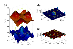
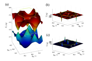
The $n$th band structure $E_{n}\left(\mathbf{q}\right)$ and the corresponding eigenvector $\phi_{n}(\mathbf{q})$ can be easily obtained by diagonalizing the Hamiltonian (3) in the strong coupling limitHamamoto2015 (see the SMSupp Sec. IV for details). We plot the band structure along the high-symmetry lines in Fig 3(a). One may notice that there is a Dirac-cone structure with a certain large gap in the vicinity of $\Gamma$ point between the bands $n=6$ and $n=7$. With the $E_{n}\left({\mathbf{q}}\right)$ and $\phi_{n}(\mathbf{q})$ available, some important quantities such as the Berry curvature, the Chern number $\mathcal{C}_{n}$ and the topological Hall conductance $\sigma_{xy}$ are readily obtained. In Fig 3(b), we plot $\sigma_{xy}$ given by the Kubo formulaHamamoto2015 (see SMSupp Sec. IV for other quantities),

where $\Xi$ is the size of the system and $f$ is the Fermi distribution function. One may notice that at zero temperature the Hall conductance is quantized to be $-1$ in the band gap between $n=6$ and $n=7$ where $E_{f}\in[-0.73,-0.61]$, which indicates a finite total Chern number, i.e., $\sum_{E_{n}<E_{f}}\mathcal{C}_{n}=\sigma_{xy}/(e^{2}/h)$.

As shown in Fig. 2, the $\rm{TmX}$ phase and the $18_{\rm B}$ phase are separated by the line $\theta=\pi/2$, where $A=0$. In both phases, there are 18 spins in one MUC. On the line $\theta=\pi/2~{}(A=0)$, these two states are degenerate (SMSupp Sec. I). One may notice that in the TmX phase $A<0$, which is thus of the easy-axis type. In the literature, several mechanisms have been proposed to stabilize merons, such as the dipole-dipole interaction ZhouEzawa2014 , the easy-plane anisotropy LinSB2015 ; HellmanHTetal2017 as well as their interplay AugustinJEetal2021 , the relative phase shifts among multiple helical spin density wavesHayamiOM2021 , and the interplay between the biquadratic interaction and the Dzyaloshinskii-Moriya interactionHayamiYambe2021 . One question naturally arises as to why the TmX phase is stable under the easy-axis anisotropy. Actually, the TmX state is rooted in the $\Gamma$ model, which has highly degenerate ground states RousochatzakisPerkins2017 . Its degeneracy is partly lifted by the Kitaev term, resulting in the degenerate TmX phase and 18_B phase (see SMSupp Sec. I and III). Moreover, as shown in Fig. 4, $\langle S_{c}^{2}\rangle=\sum_{i}\left(\mathbf{S}_{i}\cdot\mathbf{c}\right)^{2}/N$ is different in these two states. Therefore, in the presence of a finite $A$, the degeneracy is lifted. Particularly, $\langle{S_{c}^{2}}\rangle$ is larger in the TmX state, and hence when $A<0$ the TmX state is energetically favored.

Summary and Outlook. – In this work, we report our discovery of the TmX state in the high-spin Kitaev magnets and the topological effect led by such a state is demonstrated. Although the Kitaev interaction was first proposed in the spin-1/2 Kitaev honeycomb modelKitaev2006 , recent studies show that it may also exist in high-spin magnets. This offers great opportunities to study TSTs in such high-spin Kitaev magnets. Our discovery of the TmX state represents a fantastic progress in this direction and laid the foundation for the forthcoming Kitaev spintronics. On the other hand, the merons, as the classical solutions of Yang-Mills equation, were proposed as the mechanism for the quark confinement. Owing to their one half topological charge, they can only exist in pairsActor1979 ; Ezawa2011 ; PhatakLH2012 . This assessment is also supported by numerous studies in magnetsLinSB2015 ; YuKTetal2018 ; GaoJIetal2019 ; GaoRGetal2020 and photonic systemsGuoXGetal2020 . Our findings are obviously beyond this paradigm and thus extend the scope of the deconfinementSenthilVBetal2004 , which leads to our conjecture that merons with a half-integer $Q$ should be in pairs while those with an integer $Q$ can appear solely. Further studies, with Kitaev magnets as a feasible starting point, are necessary to explore such a deconfinement phenomenon.

Supplementary Material on “Triple-meron crystal in high-spin Kitaev magnets”

In this Supplementary Material, we present more details of the numerical methods, the corresponding results and the complete phase diagram. The energy optimization method and how to use it to determine the phase transition points are shown in Sec. I. In Sec. II we show how to determine the magnetic unit cell numerically. In Sec. III, we explain the origin of the TmX phase. In Sec.  IV, the details for calculating the topological charges and the topological Hall effect caused by the TmX are provided. In Sec. V, we show results from the atomistic dynamics simulations and in Sec. VI we provide the complete phase diagram. The phase diagram is determined by the ground-state energy, the spin configurations and the static spin structure factors.

Sec. I: The ground-state energy and phase-transition points by the Energy Optimization Method

Based on the spin configuration obtained by the Monte Carlo simulation, we could further use an energy optimization method to target the ground-state energy with a controllable precision. In some cases, we can derive an analytic expression for the ground-state energy. Here, we take the TmX as an example to illustrate this method.

The paradigmatic spin configuration in the TmX state, which includes three kinds of merons, is shown in Fig. 2 of the main text. As presented in Fig. sm-1, there are eighteen spins in one magnetic unit cell. For each meron, the core spin and its three NNs can be written as $(\mathbf{S}_{c}|\mathbf{S}_{i}\mathbf{S}_{j}\mathbf{S}_{k})$ for short.

In the $\bf{abc}$ coordinate system, the classical spin at site $i$ can be parameterized as

where $\vartheta_{i}\in[0,\pi]$ and $\varphi_{i}\in[0,2\pi)$. Pertaining to the core spin and its NNs in each meron, the only variable parameter is the polar angle $\vartheta_{i}$. For merons centered at site 1, 9, and 17, the auxiliary angles are found to be

and

Here, elements in the second and third rows of Eqs. (sm-5)-(sm-13) are the polar angles $\vartheta_{i}$ and azimuthal angles $\varphi_{i}$, respectively. The other six spins rely on two angles ($\vartheta_{0}$, $\varphi_{0}$), subjecting to the following relation

Hence, the Hamiltonian $\mathcal{H}$ could be recast as a multivariable function $\mathcal{F}(\vartheta_{0},\varphi_{0};\vartheta_{1},\vartheta_{2},\vartheta_{3})$ which depends on five variational parameters, and the ground-state energy is determined by minimizing $\mathcal{F}$ in the allowed parameter spaces. We emphasize that proper trial angles $(\{\vartheta_{i}\},\varphi_{0})$ guided by the Monte Carlo simulation are essential to reach the global minima of $\mathcal{F}$.

As shown in the Fig. sm-12, the classical $\rm K\Gamma{A}$ model has a rich phase diagram which contains scores of magnetically ordered phases. Here, five of them are conventional magnetic orders which also frequently appear in other spin models. In the limit of ferromagnetic (FM) Kitaev point, there are two FM phases termed FM_I phase and FM_V phase. In the former the spins lie in the $\rm\mathbf{ab}$ plane while in the latter the spins point out of the plane. Meanwhile, in the vicinity of antiferromagnetic (AFM) $\Gamma$ limit, there are an AFM_V phase for a negative $A$, and a zigzag (ZZ) phase and an in-plane 120$\rm{}^{\circ}_{I}$ phase in the case of positive $A$. We note that the ZZ phase lies in the $\rm\mathbf{ac}$ plane with a tilted angle $\alpha_{\tau}$ away from the $\rm\mathbf{a}$ axis. The ground-state energy $E_{g}$ and the polarization directions in these phases can be given analytically, which are shown in Tab. sm-1.

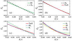
In the $\rm K\Gamma{A}$ model, when $K<0$ and $\Gamma>0$ the system is highly frustrated and many magnetic orders with a large unit cell could be stabilized. To illustrate it, we start by performing the Monte Carlo simulations along the line of $\phi=0.68\pi$ and tune the polar angle $\theta$ from $0.25\pi$ (ZZ phase) to $0.7\pi$ (12_C phase). In between, we find six distinct phases, 18_B, TmX, 48_A, 6_B, 20 and 8_B, with the increase of $\theta$. While closed forms of their ground-state energy are not available, the expression $\mathcal{F}$ that only relies on a few variational parameters could be obtained by the energy optimization method. The ground-state energy is thus targeted by minimizing $\mathcal{F}$ w.r.t. the variational parameters in the neighboring of optimal trial values. The energy of these phases is shown in Fig. sm-2, and the transition points are identified by the level-crossing points between neighboring phases.

Sec. II: Details for determing the unit cell of the TmX phase

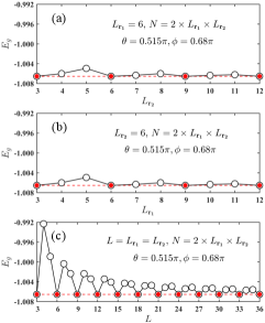
Since the magnetic unit cell of each phase is unknown aforehand, we need to determine their magnetic unit cell numerically. In Monte carlo simulations, this can be done by varying the cluster sizes and compare their ground-state energy. Here we exemplify this procedure by applying it to the TmX phase. Again we choose $\theta=0.515\pi,\phi=0.68\pi$ as the representative point. If the cluster does not match the magnetic unit cell, we will end with a higher energy than that of the true ground state in the Monte Carlo simulations. In such a case, its ground state energy may approach the true one as the size increases. Therefore we need to adjust the cluster size and compare the energy to determine the magnetic unit cell, which is shown in Fig. sm-4 with primitive lattice vetors $\mathbf{r}_{1},\mathbf{r}_{2}$ given in Fig. sm-3. In Fig. sm-4(a), we fix $L_{\mathbf{r}_{1}}=6$ and vary $L_{\mathbf{r}_{2}}$ from $3$ to $12$. We find that when $L_{\mathbf{r}_{2}}=3n$ with $n$ an integer we have the same lowest energy $E_{g}=-1.0065447701$ while the energy is higher for $L_{\mathbf{r}_{2}}=3n+1$ and $3n+2$. Moreover, the difference decreases as $n$ increases. This is well consistent with our expectation. In Fig. sm-4(b), we fix $L_{\mathbf{r}_{2}}=6$ and vary $L_{\mathbf{r}_{1}}$ from $3$ to $12$. We can find the same results as that from Fig. sm-4(a). In Fig. sm-4(c), we fix the ratio $L_{\mathbf{r}_{1}}/L_{\mathbf{r}_{2}}=1$ and vary $L_{\mathbf{r}_{1}}$ from 3 to 36. The lowest energy $E_{g}$ is at $L_{\mathbf{r}_{1}}=3n$ and it is independent of $n$. Moreover, it is the same as that in Fig. sm-4(a) and Fig. sm-4(b). These results obviously tell us the magnetic unit cell of the TmX phase has $2\times 3\times 3=18$ spins.

We want to mention that to determine the unit cell of a magnetic ordered phase, this procedure is necessary. We also apply the same method to determine other phases in the phase diagram.

Sec. III: Some formal analysis on the TmX phase

Once we know the magnetic unit cell and the corresponding magnetic order, we can do further analysis. As demonstrated in Sec. I, the variational function $\mathcal{F}(\vartheta_{0},\varphi_{0};\vartheta_{1},\vartheta_{2},\vartheta_{3})$ of $E_{g}$ in the TmX phase can be written as

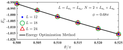
The ground state energy $E_{g}\left(=\rm{min}(\mathcal{F}/18)\right)$ is readily available by numerically optimizing such a variational function. The equations $\partial{\mathcal{F}}/\partial{\xi}=0$($\xi=\vartheta_{0},\varphi_{0},\vartheta_{1},\vartheta_{2},\vartheta_{3}$) are safisfied at the minimum and they are used to check the results. In Fig. sm-5, we compare the ground-state energy obtained by the energy optimization method and the Monte Carlo method. We find that they are well consistent, demonstrating the validity of the function $\mathcal{F}(\vartheta_{0},\varphi_{0};\vartheta_{1},\vartheta_{2},\vartheta_{3})$.

From the global phase diagram Fig. sm-12, one can see that ZZ, $18_{\mathrm{B}}$, TmX, 20, 8_B, AFM_V and 120${}^{\circ}_{\mathrm{I}}$ phases intersect at the point $\Gamma=1$ (i.e., $A=0,K=0$). The ground state of such pure $\Gamma$ model is exactly known to be classical spin liquidRousochatzakisPerkins2017 with its $E_{g}=-\Gamma$. Moreover, $E_{g}=-\Gamma$ for the $\Gamma$ model can also be obtained exactly from $\mathcal{F}(\vartheta_{0},\varphi_{0};\vartheta_{1},\vartheta_{2},\vartheta_{3})$. This further suggests that the TmX state is rooted in the $\Gamma$ model and it is one of the highly degenerate ground states of the $\Gamma$ model. To obtain a stable TmX state, a reasonable strategy is to add proper interactions to lift the degeneracy so that the TmX state becomes energetically favored. The Kitaev interaction can partly lift the degeneracy and the degenerate TmX and 18_B become the ground states. As we have shown in the main text, the degeneracy of the TmX and 18_B is further lifted by the single-ion anisotropy $A$. For a negative $A$, the TmX state is energetically favored.

Sec. IV: Topological Charge and Topological Hall Effect

First, we discuss briefly how to calculate the topological charges $Q$ of the merons in our lattice model. The definition was given by Berg and LüscherBergLuscher1981 , which is illustrated in Fig. sm-6. Actually, in a lattice the topological charge can be obtained by summing up the solid angle on every elementary triangle. For this purpose, the hexagon of each meron is splitted into six equilateral triangles, each is formed by a core spin and its two next-nearest neighbors. Among these six triangles, three of them contain an additional spin (the nearest neighbor of the core), which further divides the equilateral triangle into three isosceles triangles. The solid angle for each triangle is thus calculated following the definition given by Berg and LüscherBergLuscher1981 . In our work we present the values of the topological charges up to six digits for simplicity although the numerical errors are of the order $10^{-14}$ or smaller.

In Fig. sm-7 we plot the topological charges $Q$ of the three merons and their summation as a function of $\theta$. Although the outmost spins might be driven off $\mathbf{ab}$-plane, we can see that $Q_{\mathcal{B}}$ and $Q_{\mathcal{C}}$ are still close to $\pm 1/2$ and $Q_{\mathcal{A}}$ is roughly 1. Importantly, their summation is always 1.0. We want to mention that in the TmX phase we can find parameters with the topological charges of $Q_{\mathcal{A}},Q_{\mathcal{B}},Q_{\mathcal{C}}$ much closer to their theoretical values. For example, at $\theta=0.515\pi,\phi=0.656\pi$, $Q_{\mathcal{A}}=0.999881$, $Q_{\mathcal{B}}=0.500058$ and $Q_{\mathcal{C}}=-0.499939$, respectively. Moreover, due to the quadratic form of our model, a degenerate ground state is obtained by flipping all the spins. Under this transformation, a straightforward conclusion is that the topological charges of corresponding merons are sign-reversed.

Next, we discuss the details about calculating topological Hall effect (THE). Since there is no THE in the meron-antimeron crystalsHayamiOM2021 , the THE caused by the TmX is highly nontrivial for the merons crystals. The double-exchange model used in main text means the coupling between itinerant electrons and the local magnetization is much larger than the hoping amplitude, so the spin of itinerant electron should be parallel to the direction of local magnetization $\mathbf{S}_{i}$. Hence, the energy of Kondo coupling term turns to be a constant. By defining a rotation matrix $U_{i}$ on each site which rotates the eigenvector of the itinerant electron from $\sigma_{z}$ to $\bm{\sigma}\cdot\mathbf{S}_{i}$, the above Hamiltonian can be transformed to a spinless free-fermion modelHamamoto2015 :

where

and

with $\bar{\theta}_{i}$ and $\bar{\phi}_{i}$ the corresponding polar and azimuthal angle of the on-site magnetization $\mathbf{S}_{i}$.

The band structure $E_{n}\left({\mathbf{q}}\right)$ as well as wave functions $\phi_{n}\left(\mathbf{q}\right)$ can be directly obtained through the above effective Hamiltonian. The topological property of a band can be determined through its Chern number $\mathcal{C}_{n}$ , which by definition is the integration of the Berry curvature $\bm{\Sigma}$ over the first Brillouin zone:

with $\mathbf{A}(\mathbf{q})=-i\langle\phi_{n}(\mathbf{q})|\nabla_{\mathbf{q}}|\phi_{n}(\mathbf{q})\rangle$ the Berry connection.

The Chern number of the first 9 bands presented in main text are 0, 0, 0, 1, 0, -2, 2, 1, 2. Since there is no band gap between 7-8 band and between the 8-9 bands, we focus on the 4-5 and 6-7 bands. Fig. sm-8 and Fig. sm-9 shows the full band structure and Berry curvature of selected bands. There is a clear Dirac cone structure with certain large gap in the vicinity of $\Gamma$ point between 6 and 7 bands. As a results, one can see that the Berry curvature mainly concentrates around $\Gamma$ point (Fig. sm-8). As a contrast, there are two Dirac cones at $\Gamma$ and $K_{2}$ points between 4 and 5 bands resulting in very narrow global gap, and the Berry curvature dominates around $\Gamma$ and $K_{2}$ (Fig. sm-9).

One may notice that the quantized Hall conductance shown in the main text is just the total Chern number when the chemical potential is inside the gap between the bands 6 and 7, i.e., $\sigma_{xy}=e^{2}/h\sum_{E_{n}<E_{f}}\mathcal{C}_{n}$, since the Berry curvature could be equivalently obtained through Kubo formula as well. There is also a very narrow conductance platform between the bands 4 and 5, due to the tiny global gap there.

Sec. V: Spin dynamics simulations

Since the TmX state is found in the ground-state phase diagram, an important question to be answered is whether we can obtain such state experimentally. While Monte Carlo simulation is an elaborate and powerful metheod for equilibrium state problems, the dynamics of magnetic properties like: domain-wall motion, Hysteresis loop, pining-depinning problem, etc., are usually treated with Landau-Lifshitz-Gilbert equationLandau1935 ; Gilbert2004 . To this end, we perform atomistic spin-dynamics simulations on field-cooling process of TmX state. Here, we choose again the representative point $\theta=0.515\pi,\phi=0.68\pi$.

The Landau-Lifshitz-Gilbert (LLG) equation is numerically solved in the xyz coordinate system:

with

the effective field felt by $\mathbf{S}_{i}$, $\alpha^{\prime}$ a dimensionless damping factor and $\mathbf{h}_{ext}^{c}$ an external magnetic field along $\mathbf{c}$ direction. For finite temperatures, a stochastic fluctuation field $\mathbf{h}^{fl}$ is then added to the effective field to act as the thermal noise, which should have a zero average value and be uncorrelated in spin component, space and time:

with $\epsilon^{2}=2\alpha^{\prime}k_{B}\mathcal{T}$ and $\mathcal{T}$ the temperature determining the strength of thermal fluctuations. In our simulation, we set $k_{B}=\hbar=1$ (a dimensionless system), $\alpha^{\prime}=0.01$ (different values of $\alpha^{\prime}$ have also been tested) and solve the LLG equation using the fourth-order Runge–Kutta method on a $288\times 288\times 2$ honeycomb lattice. $6\times 10^{6}$ iterations are performed between every two successive temperatures.

As we have already noticed, the TmX state is degenerate but with an opposite $Q$ under the transformation $\bf{S}\rightarrow-\bf{S}$. These two states might appear simultaneously and annihilate each other when starting from a random initial state. Such a degeneracy can be easily lifted by applying an external magnetic field $h_{ext}^{c}$ along the $c$-axis. As shown in Fig. sm-10(a)-(c), one can already find the TmX state when the temperature $\mathcal{T}=0.01$. As $\mathcal{T}$ decreases, the TmX state becomes more clear, suggesting the field cooling is indeed effective to obtain a stable TmX state (Supplementary Movie Sabc). However, one may notice that there are two kinds of TmX states with their core spins on different sublattices, say, a and b, which are separated by narrow domains (Fig. sm-10(c) and Fig. sm-10(d)). Such a phenomenon arises from the bipartite nature of the honeycomb lattice. To eliminate such domains, it is necessary to lift the degeneracy further. In our numerical simulations, a simple strategy is to change $A$ on one sublattice, say a, to $\alpha A$ with $\alpha$ equal to, for example, $0.9$. We want to mention that in experiments one can break the symmetry of the lattice by applying strain. The corresponding results are shown in Fig. sm-10(e)-(h). Though there are still domains at $\mathcal{T}=0.01$, one can find a nearly perfect TmX state at $\mathcal{T}=0.001$ (Supplementary Movie Sefg). We want to stress that lifting such degeneracy is definitely helpful to eliminate domains but the effect depends on $\alpha$ as well as the initial configuration. As shown in Fig. sm-11, the parameters and simulation details in Fig. sm-11 and Fig. sm-10 are the same except that the random initial configuration is different. However, in Fig. sm-11(g) there are still domains. Even though, the effect of lifting the degeneracy can be demonstrated by counting the number of merons with their cores on the different sublattice, say $N_{a}$ or $N_{b}$. In Fig. sm-11(c) where $\mathcal{T}=0.001$, $N_{a}:N_{b}=7524:7328$, which is very close to $1:1$. This ratio again evidences the degeneracy of the TmX state. As we change the coefficient of the single-ion anisotropy $A$ on the sublattice a to $0.9A$ in Fig. sm-11(e)-(h), at $\mathcal{T}=0.001$ (Fig. sm-11(g)), the region of the energetically favored Tmx state is obviously increased, i.e., $N_{a}:N_{b}=12337:3937$. One may naively expect that core spins on the $b$ sublattice is energetically favored because $\alpha<1.0$ and $A<0$. Actually, this is not true. Changing $\alpha$ simultaneously changes the spin directions of NNs and NNNs and one can not just compare the energy of the core spins. We confirm the core spins prefer staying on the $a$ sublattice by the Monte Carlo simulations.

Sec. VI: Complete phase diagram, Spin configurations and static spin structure factors

In this section, we show the complete phase diagram, the spin configurations and the corresponding static spin structure factors ${{\mathcal{F}}_{\bf{q}}^{\xi\xi}}=\frac{1}{N}\sum_{ij}e^{i{\bf{q}}\cdot(\bf{R}_{i}-\bf{R}_{j})}\langle{S_{i}^{{\xi}}S_{j}^{\xi}}\rangle$ ($\xi={\bf{a,b,c}}$).

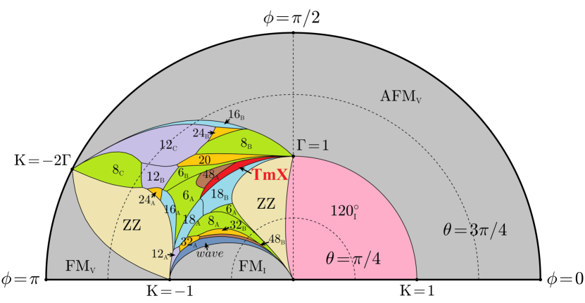
The complete phase diagram of the $\rm K\Gamma{A}$ model is shown in Fig. sm-12 as a semicircle plot. The radial distance represents $\theta$ and the polar angle represents $\phi$. In the region $\pi/2<\phi<\pi$, the model is highly frustrated and a large number of phases are found. The number in the phase diagram marks the number of spins in one magnetic unit cell and the subscripts A, B, C and D are used to distinguish different phases marked by the same number. The phase transitions of all the ordered phases are of the first order except that the transitions to the wave phase is unclear. Note that on the line $\theta=\pi$, where $K=0$ and $\Gamma=0$, the Hamiltonian is decoupled and then become trivial. From the symmetry, it is ready to know that the line $\phi=\pi$, or equivalently $\phi=0$, is the phase transition line.

In the following, we will show the spin configuration and the static spin structure factors of each phase. We will not show the five phases discussed in Sec. I since they are common and their properties are well known in magnets. For simplicity, we choose one representive point in each phase to illustrate the spin structure, which are shown in Fig. sm-14-Fig. sm-26 with the phase name and corresponding parameters given in the caption. In each figure, the spin configurations are shown on the left panels and the corresponding static spin structure factors are on the right panels. On the right panel, the $a,b$ or $c$ in the subfigures marks the spin component and the right bottom subfigures show the summation of all three components. Since there two regions belonging to the 6_A phase, we choose one point in each region and plot them in Fig. sm-16 and Fig. sm-16. The magnetic unit cell of the $\it{wave}$ phase is rather complex. It may vary as a function of $\theta$ and $\phi$. At present we can not draw a reliable conclusion. The two figures sm-35 and sm-36 are plotted just for reference.

References

- (1) Ioannis Rousochatzakis and Natalia B. Perkins, Classical Spin Liquid Instability Driven By Off-Diagonal Exchange in Strong Spin-Orbit Magnets, Phys. Rev. Lett. 118, 147204 (2017).
- (2) B. Berg and M. Lüscher, Definition and statistical distributions of a topological number in the lattice O(3) -model. Nucl. Phys. B 190, 412-424 (1981).
- (3) S. Hayami, T. Okubo, and Y. Motome, Phase shift in skyrmion crystals, Nat. Commun. 12, 6927 (2021).
- (4) K. Hamamoto, M. Ezawa, and N. Nagaosa, Quantized topological Hall effect in skyrmion crystal, Phys. Rev. B 92, 115417 (2015).
- (5) L. D. Landau and E. Lifschitz, On the theory of magnetic permeability in ferromagnetic bodies. Phys. Z. Sowjetunion 8, 153 (1935).
- (6) T. L. Gilbert, A phenomenological theory of damping in ferromagnetic materials. IEEE Trans. Magn. 40, 3443 (2004).