Triple-charm molecular states composed of $D^{*}D^{*}D$ and $D^{*}D^{*}D^{*}$

As important members of the hadron family, exotic states have always interested both theoreticians and experimentalists. By definition, exotic states contain more complex quark and gluon contents than the conventional $q\bar{q}$ mesons and $qqq$ baryons. Given their peculiar nature, studies of exotic states have been a hot topic in hadron physics.

Among the various exotic states, hadronic molecules are quite distinct. They are loosely bound states composed of two or several conventional hadrons and provide a good laboratory to study hadron structure and nonperturbative strong interactions at hadronic level. In 2003, the $BABAR$ Collaboration observed a charmed-strange state $D_{s0}^{*}(2317)$ in the $D_{s}\pi^{0}$ channel BaBar:2003oey . Soon after, the CLEO Collaboration not only confirmed its existence , but also found a new charmed-strange state $D_{s1}^{\prime}(2460)$ in the $D_{s}^{*}\pi^{0}$ mass spectrum CLEO:2003ggt . In the same year, the Belle Collaboration reported a hidden-charm state $X(3872)$ in the $J/\psi\pi^{+}\pi^{-}$ channel Belle:2003nnu . The $D_{s0}^{*}(2317)$, $D_{s1}^{\prime}(2460)$, and $X(3872)$ states have two peculiar features. The first is that their masses are about 100 MeV below the potential model predictions, which implies that it is difficult to categorize them as conventional mesons. The second is that $D_{s0}^{*}(2317)$, $D_{s1}^{\prime}(2460)$, and $X(3872)$ are close to and lower than the $DK$, $D^{*}K$, and $D\bar{D}^{*}$ thresholds, which strongly hints at their molecular nature. Although there are still many controversies, hadronic molecules are one of the most popular interpretations of these exotic hadrons Barnes:2003dj ; Xie:2010zza ; Guo:2006fu ; Faessler:2007gv ; Feng:2012zze ; Faessler:2007us ; Zhang:2006ix ; Swanson:2003tb ; Wong:2003xk ; Liu:2009qhy ; Lee:2009hy ; Altenbuchinger:2013vwa . The observations of $D_{s0}^{*}(2317)$, $D_{s1}^{\prime}(2460)$, and $X(3872)$ opened a new era in searches for exotic states. In the following years, a plethora of hidden-charm $XYZ$ and $P_{c}$ states were observed in experiments (for reviews, see Refs. Chen:2016qju ; Liu:2013waa ; Yuan:2018inv ; Olsen:2017bmm ; Guo:2017jvc ; Hosaka:2016pey ; Brambilla:2019esw ).

Very recently, the LHCb Collaboration observed a $T_{cc}^{+}$ state in the $D^{0}D^{0}\pi^{+}$ channel LHCb:2021vvq ; LHCb:2021auc , whose mass and width obtained from a Breit-Wigner fit are

$$\begin{split}m_{\rm BW}=&(m_{D^{*+}}+m_{D^{0}})-273\pm 61\pm 5^{+11}_{-14}\;{\rm keV},\\ \Gamma_{\rm BW}=&410\pm 165\pm 43^{+18}_{-38}\;{\rm keV}.\end{split}$$

(1)

On the other hand, the pole position is given as LHCb:2021auc

$$\begin{split}m_{\rm pole}=&(m_{D^{*+}}+m_{D^{0}})-360\pm 40^{+4}_{-0}\;{\rm keV},\\ \Gamma_{\rm pole}=&48\pm 2^{+0}_{-14}\;{\rm keV}.\end{split}$$

(2)

From the decay products of $T_{cc}^{+}$, one can infer its minimum quark component to be $cc\bar{u}\bar{d}$. Since the mass of the $T_{cc}^{+}$ is very close to the $D^{*}D$ threshold, it could well be interpreted as a $D^{*}D$ molecular state Li:2021zbw ; Ren:2021dsi ; Chen:2021vhg ; Dai:2021vgf ; Feijoo:2021ppq ; Wu:2021kbu as predicted in many previous works  Molina:2010tx ; Li:2012ss ; Liu:2019stu ; Xu:2017tsr . As early as in the 1980s, the likely existence of stable tetraquark states has attracted the interests of theorists Ader:1981db ; Ballot:1983iv ; Lipkin:1986dw ; Zouzou:1986qh ; Heller:1986bt ; Carlson:1987hh . Latter, various models with different quark-quark interactions were employed to study the mass spectrum of tetraquark states with the $QQ\bar{q}\bar{q}$ configuration Manohar:1992nd ; Pepin:1996id ; Vijande:2006jf ; Ebert:2007rn ; Vijande:2013qr ; Karliner:2017qjm ; Eichten:2017ffp ; Richard:2018yrm ; Park:2018wjk ; Hernandez:2019eox . It should be noted that the $T_{cc}^{+}$ is the first observed double-charm exotic state. It is interesting to note that the decay width obtained from the Breit-Wigner fit and that derived from the pole position are quite different. The latter strongly supports its nature being a hadronic molecule of $DD^{*}$, as stressed, e.g., in Ref. Ling:2021bir .

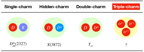
The single-charm, hidden-charm, and double-charm molecular candidates have been established in experiments. In Fig. 1, we choose the $D_{s0}^{*}(2317)$, $X(3872)$, and $T_{cc}^{+}$ states as examples and present the corresponding possible substructure. However, until now, there was no signal of triple-charm molecular states. In the future, experimental searches for triple-charm molecular states will be an interesting topic in exploring exotic hadrons.

In this work, we investigate the likely existences of triple-charm molecular states composed of $D^{*}D^{*}D$ and $D^{*}D^{*}D^{*}$. There are three reasons for studying such systems. First, we notice that single- and double-charm molecular candidates in Fig. 1 contain one and two charmed mesons, respectively. Thus it is natural to ask whether there exist hadronic molecular states composed of three charmed mesons. Second, the observation of the $T_{cc}^{+}$ state provides a way to fix the interaction between two charmed mesons. In Ref. Wu:2021kbu , we successfully reproduced the binding energy of the $T_{cc}^{+}$ state, with the $DD^{*}$ interaction provided by the one-boson-exchange (OBE) model. This makes the numerical results more reliable when dealing with systems containing more charmed mesons in the following study. Third, in Ref. Wu:2021kbu , we have studied the $DDD^{*}$ system and found that it has a $I(J^{P})=\frac{1}{2}(1^{-})$ bound state solution. Compared with the $DDD^{*}$ system, the $D^{*}D^{*}D$ and $D^{*}D^{*}D^{*}$ systems can have more spin configurations. Therefore, it is likely that there exist more hadronic molecular states in the $D^{*}D^{*}D$ and $D^{*}D^{*}D^{*}$ systems.

In the past several years, the LHCb Collaboration has achieved great success in discovering exotic states, including several $P_{c}$ states LHCb:2015yax ; LHCb:2019kea , $P_{cs}$ LHCb:2020jpq , $X_{0,1}(2900)$ LHCb:2020bls ; LHCb:2020pxc , and $X(6900)$ LHCb:2020bwg . These observations demonstrated the capacity of the LHCb detector in searching for exotic states. With the upgrade of the LHCb detector LHCb:2018roe , one can expect that more exotic states will be observed in the future. The predictions of molecular states with the configurations of $D^{*}D^{*}D$ and $D^{*}D^{*}D^{*}$ may inspire more experimental works along this line.

This paper is organized as follows. In Sec. II, we introduce the interactions between $D^{*}$ and $D^{(*)}$ and present the details of the Gussian expansion method. Next in Sec. III, we present the binding energies and root-mean-square radii of the $D^{*}D^{*}D$ and $D^{*}D^{*}D^{*}$ systems. Finally, this paper ends with a short summary in Sec. IV.

In order to study the $D^{*}D^{*}D$ and $D^{*}D^{*}D^{*}$ systems, we should first derive the effective potentials of the $D^{*}$-$D^{*}$ and $D$-$D^{*}$ pairs. For this purpose, we adopt the OBE model of Ref. Liu:2019stu . In the OBE model, the $D^{*}$-$D^{(*)}$ interactions occur by the scattering process as shown in Fig. 2, where we should consider the exchanges of $\pi$, $\sigma$, $\rho$, and $\omega$ mesons. Then, in the momentum space, the effective potential related to the scatting amplitude can be written as

$$V^{h_{1}h_{2}\to h_{3}h_{4}}({\bf q})=-\frac{{\cal M}^{h_{1}h_{2}\to h_{3}h_{4}}({\bf q})}{\sqrt{\prod_{i}2m_{i}\prod_{i}2m_{f}}},$$

(3)

where ${\cal M}^{h_{1}h_{2}\to h_{3}h_{4}}({\bf q})$ is the scattering amplitude. The $m_{i}$ and $m_{f}$ are masses of the initial and final states. To take into the finite size of the exchanged mesons, a monopole form factor is introduced

$${\cal F}(q^{2},m_{E}^{2})=\frac{\Lambda^{2}-m_{E}^{2}}{\Lambda^{2}-q^{2}},$$

(4)

where $q$ and $m_{E}$ are the mass and momentum of the exchanged meson, respectively. The effective potentials in the coordinate space can be obtained by the following Fourier transformation

$$V^{h_{1}h_{2}\to h_{3}h_{4}}({\bf r})=\int\frac{{\rm d}^{3}{\bf q}}{(2\pi)^{3}}{\rm e}^{i{\bf q}\cdot{\bf r}}V^{h_{1}h_{2}\to h_{3}h_{4}}({\bf q}){\cal F}^{2}(q^{2},m_{E}^{2}).$$

(5)

In the following, we present the effective potentials of the $D^{*}$-$D^{(*)}$ interactions explicitly, i.e.,

$$\begin{split}V^{DD^{*}\to DD^{*}}=&-g_{\sigma}^{2}{\cal O}_{1}Y_{\sigma}+\frac{1}{2}\beta^{2}g_{V}^{2}{\cal O}_{1}\left({\cal C}_{1}(I)Y_{\rho}+{\cal C}_{0}(I)Y_{\omega}\right),\\ V^{DD^{*}\to D^{*}D}=&\frac{g^{2}}{3f_{\pi}^{2}}({\cal O}_{2}\hat{\cal P}+{\cal O}_{3}\hat{\cal Q}){\cal C}_{1}^{\prime}(I)Y_{\pi 1}\\ &+\frac{2}{3}\lambda^{2}g_{V}^{2}(2{\cal O}_{2}\hat{\cal P}-{\cal O}_{3}\hat{\cal Q})\left({\cal C}_{1}^{\prime}(I)Y_{\rho 1}+{\cal C}_{0}^{\prime}(I)Y_{\omega 1}\right),\\ V^{DD^{*}\to D^{*}D^{*}}=&\frac{g^{2}}{3f_{\pi}^{2}}({\cal O}_{4}\hat{\cal P}+{\cal O}_{5}\hat{\cal Q}){\cal C}_{1}(I)Y_{\pi 2}\\ &+\frac{2}{3}\lambda^{2}g_{V}^{2}(2{\cal O}_{4}\hat{\cal P}-{\cal O}_{5}\hat{\cal Q})\left({\cal C}_{1}(I)Y_{\rho 2}+{\cal C}_{0}(I)Y_{\omega 2}\right),\\ V^{D^{*}D^{*}\to D^{*}D^{*}}=&-g_{\sigma}^{2}{\cal O}_{6}Y_{\sigma}+\frac{1}{2}\beta^{2}g_{V}^{2}{\cal O}_{6}\left({\cal C}_{1}(I)Y_{\rho}+{\cal C}_{0}(I)Y_{\omega}\right)\\ &-\frac{g^{2}}{3f_{\pi}^{2}}({\cal O}_{7}\hat{\cal P}+{\cal O}_{8}\hat{\cal Q}){\cal C}_{1}(I)Y_{\pi}\\ &-\frac{2}{3}\lambda^{2}g_{V}^{2}(2{\cal O}_{7}\hat{\cal P}-{\cal O}_{8}\hat{\cal Q})\left({\cal C}_{1}(I)Y_{\rho}+{\cal C}_{0}(I)Y_{\omega}\right).\\ \end{split}$$

(6)

In Eq. (6), the ${\cal O}_{i}$’s are spin-dependent operators, which are defined as

$$\begin{split}{\cal O}_{1}=&{\bm{\epsilon}}_{4}^{\dagger}\cdot{\bm{\epsilon}}_{2},\\ {\cal O}_{2}=&{\bm{\epsilon}}_{3}^{\dagger}\cdot{\bm{\epsilon}}_{2},\\ {\cal O}_{3}=&S({\bf r},{\bm{\epsilon}}_{3}^{\dagger},{\bm{\epsilon}}_{2}),\\ {\cal O}_{4}=&{\bm{\epsilon}}_{3}^{\dagger}\cdot(i{\bm{\epsilon}}_{4}^{\dagger}\times{\bm{\epsilon}}_{2}),\\ {\cal O}_{5}=&S({\bf r},{\bm{\epsilon}}_{3}^{\dagger},i{\bm{\epsilon}}_{4}^{\dagger}\times{\bm{\epsilon}}_{2}),\\ {\cal O}_{6}=&({\bm{\epsilon}}_{3}^{\dagger}\cdot{\bm{\epsilon}}_{1})({\bm{\epsilon}}_{4}^{\dagger}\cdot{\bm{\epsilon}}_{2}),\\ {\cal O}_{7}=&({\bm{\epsilon}}_{3}^{\dagger}\times{\bm{\epsilon}}_{1})\cdot({\bm{\epsilon}}_{4}^{\dagger}\times{\bm{\epsilon}}_{2}),\\ {\cal O}_{8}=&S({\bf r},{\bm{\epsilon}}_{3}^{\dagger}\times{\bm{\epsilon}}_{1},{\bm{\epsilon}}_{4}^{\dagger}\times{\bm{\epsilon}}_{2}),\\ \end{split}$$

(7)

where

$$S({\bf r},{\bf a},{\bf b})=\frac{3({\bf a}\cdot{\bf r})({\bf b}\cdot{\bf r})}{r^{2}}-{\bf a}\cdot{\bf b}$$

(8)

is the tensor operator. Here, ${\bm{\epsilon}}_{i}$ ($i=1,2$) and ${\bm{\epsilon}}^{\dagger}_{i}$ ($i=3,4$) are initial and final polarization vectors of the $D^{*}$ mesons, respectively, and $C_{0}^{(\prime)}(I)$ and $C_{1}^{(\prime)}(I)$ are flavor-dependent factors given by

$$\begin{split}&{\cal C}_{1}(0)=-\frac{3}{2},~{}{\cal C}_{1}^{\prime}(0)=+\frac{3}{2},~{}{\cal C}_{0}(0)=+\frac{1}{2},~{}{\cal C}_{0}^{\prime}(0)=-\frac{1}{2},\\ &{\cal C}_{1}(1)=+\frac{1}{2},~{}{\cal C}_{1}^{\prime}(1)=+\frac{1}{2},~{}{\cal C}_{0}(1)=+\frac{1}{2},~{}{\cal C}_{0}^{\prime}(1)=+\frac{1}{2}.\end{split}$$

(9)

The function $Y_{i}$ in Eq. (6) is written as¹¹1 In momentum space, the effective potentials share a common part, i.e., $$V({\bf q})=\frac{1}{{\bf q}^{2}+m_{E}^{2}-{q^{0}}^{2}},$$ (10) where the $q^{0}$ is energy component of the exchange momentum, whose explicit expression could be found in Ref. Li:2012ss . Without a form factor, the Fourier transformation of Eq. (10) is $$\begin{split}V({\bf r})=&\int\frac{{\rm d}^{3}{\bf q}}{(2\pi)^{3}}{\rm e}^{i{\bf q}\cdot{\bf r}}\frac{1}{{\bf q}^{2}+m_{E}^{2}-{q^{0}}^{2}}\\ &=\frac{1}{4\pi r}{\rm e}^{-\sqrt{m_{E}^{2}-{q^{0}}^{2}}r}.\end{split}$$ (11) After introducing the form factor, the Fourier transformation is $$\begin{split}V({\bf r})=&\int\frac{{\rm d}^{3}{\bf q}}{(2\pi)^{3}}{\rm e}^{i{\bf q}\cdot{\bf r}}\frac{1}{{\bf q}^{2}+m_{E}^{2}-{q^{0}}^{2}}{\cal F}^{2}(q^{2},m_{E}^{2}).\end{split}$$ (12) After performing the integration, one could obtain the function $Y_{i}$ given in Eq. (13).

$$Y_{i}=\frac{{\rm e}^{-m_{Ei}r}}{4\pi r}-\frac{{\rm e}^{-\Lambda_{i}r}}{4\pi r}-\frac{\Lambda_{i}^{2}{\rm e}^{-\Lambda_{i}r}}{8\pi\Lambda_{i}}+\frac{m_{Ei}^{2}{\rm e}^{-\Lambda_{i}r}}{8\pi\Lambda_{i}}$$

(13)

with $\Lambda_{i}=\sqrt{\Lambda^{2}-q_{i}^{2}}$ and $m_{Ei}=\sqrt{m_{E}^{2}-q_{i}^{2}}$. The $q_{i}$ is the energy component of the exchanged momentum. We employ $q_{1}=m_{D^{*}}-m_{D}$ and $q_{2}=(m_{D^{*}}^{2}-m_{D}^{2})/(4m_{D^{*}})$ for the $DD^{*}\to D^{*}D$ and $DD^{*}\to D^{*}D^{*}$ processes, respectively. The operators $\hat{\cal P}$ and $\hat{\cal Q}$ only act on $Y_{i}$ and the expressions are

$$\hat{\cal P}=\frac{1}{r^{2}}\frac{\partial}{\partial r}r^{2}\frac{\partial}{\partial r},~{}~{}~{}\hat{\cal Q}=r\frac{\partial}{\partial r}\frac{1}{r}\frac{\partial}{\partial r}.$$

(14)

To evaluate the above potentials, we also need the values of the coupling constants and the masses of the mesons, which are collected in Table 1.

To solve the three-body Schrödinger equation, we employ the Gaussian expansion method Hiyama:2003cu ; Hiyama:2012sma , which was widely used in studies of baryon systems Yoshida:2015tia ; Yang:2019lsg ; Yang:2017qan , multiquark states Yang:2021izl ; Yang:2020fou ; Wang:2019rdo ; Lu:2021kut ; Lu:2020cns , and multibody hadronic molecular states Wu:2019vsy ; Wu:2020rdg ; Wu:2020job ; Wu:2021kbu ; Wu:2021gyn (for reviews on this latter topic, see, e.g., Refs. Wu:2021ljz ; Wu:2021dwy ). The three-body Schrödinger equation reads

$$\left[\hat{T}+V(r_{1})+V(r_{2})+V(r_{3})\right]\Psi_{JM}=E\Psi_{JM},$$

(15)

where $\hat{T}$ is the kinetic energy operator, and $V(r_{1})$, $V(r_{2})$, and $V(r_{3})$ are pairwise potentials. $\Psi_{JM}$ is the total wave function, which can be written as

$$\Psi_{JM}=\sum_{c,\alpha}C_{c,\alpha}\Psi_{JM}^{(c,\alpha)},$$

(16)

where

$$\begin{split}\Psi_{JM}^{(c,\alpha)}=H_{t,T}^{c}\left[\chi_{s,S}^{c}\left[\phi_{nl}({\bf r}_{c})\phi_{NL}({\bf R}_{c})\right]_{\lambda}\right]_{JM}\end{split}$$

(17)

is the basis, and $C_{c,\alpha}$ is the coefficient of the corresponding basis, which can be obtained by the Rayleigh-Ritz variational method. The $c$ ($c=1,2,3$) represents the three channels in Fig. 3 and $\alpha=\{tT,sS,nN,lL\lambda\}$ is the quantum number of the basis. $H_{t,T}^{c}$ is the flavor wave function, where $t$ is isospin in the ${\bf r}_{c}$ degree of freedom and $T$ is the total isospin. $\chi_{s,S}^{c}$ is the spin wave function, where the $s$, $S$ are spin in the ${\bf r}_{c}$ degree of freedom and total spin, respectively. $\phi_{nlm_{l}}({\bf r}_{c})$ and $\phi_{NLM_{L}}({\bf R}_{c})$ are spatial wave functions, which read

$$\begin{split}\phi_{nlm_{l}}({\bf r}_{c})=&N_{nl}r_{c}^{l}e^{-\nu_{n}r_{c}^{2}}Y_{lm}(\hat{\bf r}_{c}),\\ \phi_{NLM_{L}}({\bf R}_{c})=&N_{NL}R_{c}^{L}e^{-\lambda_{N}R_{c}^{2}}Y_{LM}(\hat{\bf R}_{c}),\\ \end{split}$$

(18)

where $N_{nl}$ and $N_{NL}$ are normalization constants. In Eq. (18), The ${\bf r}_{c}$ and ${\bf R}_{c}$ are Jacobi coordinates, and $\nu_{n}$ and $\lambda_{N}$ are Gaussian ranges. After the above preparations, we can calculate the kinetic, potential, and normalization matrix elements (see Refs. Hiyama:2003cu ; Brink:1998as for more details), i.e.,

$$\begin{split}T^{ab}_{\alpha\alpha^{\prime}}=&\langle\Psi_{JM}^{(a,\alpha)}|\hat{T}|\Psi_{JM}^{(b,\alpha^{\prime})}\rangle,\\ V^{ab}_{\alpha\alpha^{\prime}c}=&\langle\Psi_{JM}^{(a,\alpha)}|V({r_{c}})|\Psi_{JM}^{(b,\alpha^{\prime})}\rangle,\\ N^{ab}_{\alpha\alpha^{\prime}}=&\langle\Psi_{JM}^{(a,\alpha)}|\Psi_{JM}^{(b,\alpha^{\prime})}\rangle.\end{split}$$

(19)

Then, Eq. (15) could be further expressed as the following general eigenvalue equation:

$$\left(T^{ab}_{\alpha\alpha^{\prime}}+\sum\limits_{c=1}^{3}V^{ab}_{\alpha\alpha^{\prime}c}\right)C_{b,\alpha^{\prime}}=EN^{ab}_{\alpha\alpha^{\prime}}C_{b,\alpha^{\prime}}.$$

(20)

References

- (1) B. Aubert et al. [BaBar], Observation of a narrow meson decaying to at a mass of 2.32 GeV/, Phys. Rev. Lett. 90, 242001 (2003).
- (2) D. Besson et al. [CLEO], Observation of a narrow resonance of mass 2.46 GeV/ decaying to and confirmation of the state, Phys. Rev. D 68, 032002 (2003), [erratum: Phys. Rev. D 75, 119908 (2007)].
- (3) S. K. Choi et al. [Belle], Observation of a narrow charmonium-like state in exclusive decays, Phys. Rev. Lett. 91, 262001 (2003).
- (4) T. Barnes, F. E. Close and H. J. Lipkin, Implications of a molecule at 2.32 GeV, Phys. Rev. D 68, 054006 (2003).
- (5) Z. X. Xie, G. Q. Feng and X. H. Guo, Analyzing in the molecule picture in the Beth-Salpeter approach, Phys. Rev. D 81, 036014 (2010).
- (6) F. K. Guo, P. N. Shen, H. C. Chiang, R. G. Ping and B. S. Zou, Dynamically generated heavy mesons in a heavy chiral unitary approach, Phys. Lett. B 641, 278-285 (2006).
- (7) A. Faessler, T. Gutsche, V. E. Lyubovitskij and Y. L. Ma, Strong and radiative decays of the meson in the -molecule picture, Phys. Rev. D 76, 014005 (2007).
- (8) G. Q. Feng, X. H. Guo and Z. H. Zhang, Studying the molecular structure of in the Bethe-Salpeter approach, Eur. Phys. J. C 72, 2033 (2012).
- (9) A. Faessler, T. Gutsche, V. E. Lyubovitskij and Y. L. Ma, molecular structure of the meson, Phys. Rev. D 76, 114008 (2007).
- (10) Y. J. Zhang, H. C. Chiang, P. N. Shen and B. S. Zou, Possible -wave bound-states of two pseudoscalar mesons, Phys. Rev. D 74, 014013 (2006).
- (11) E. S. Swanson, Short range structure in the , Phys. Lett. B 588, 189-195 (2004).
- (12) C. Y. Wong, Molecular states of heavy quark mesons, Phys. Rev. C 69, 055202 (2004).
- (13) X. Liu, Z. G. Luo, Y. R. Liu and S. L. Zhu, and Other Possible Heavy Molecular States, Eur. Phys. J. C 61, 411-428 (2009).
- (14) I. W. Lee, A. Faessler, T. Gutsche and V. E. Lyubovitskij, as a molecular state in a potential model, Phys. Rev. D 80, 094005 (2009).
- (15) M. Altenbuchinger, L. S. Geng and W. Weise, Scattering lengths of Nambu-Goldstone bosons off mesons and dynamically generated heavy-light mesons, Phys. Rev. D 89, no.1, 014026 (2014).
- (16) H. X. Chen, W. Chen, X. Liu and S. L. Zhu, The hidden-charm pentaquark and tetraquark states, Phys. Rept. 639, 1-121 (2016).
- (17) X. Liu, An overview of new particles, Chin. Sci. Bull. 59, 3815-3830 (2014).
- (18) C. Z. Yuan, The states revisited, Int. J. Mod. Phys. A 33, no.21, 1830018 (2018).
- (19) S. L. Olsen, T. Skwarnicki and D. Zieminska, Nonstandard heavy mesons and baryons: Experimental evidence, Rev. Mod. Phys. 90, no.1, 015003 (2018).
- (20) F. K. Guo, C. Hanhart, U. G. Meißner, Q. Wang, Q. Zhao and B. S. Zou, Hadronic molecules,” Rev. Mod. Phys. 90, no.1, 015004 (2018).
- (21) A. Hosaka, T. Iijima, K. Miyabayashi, Y. Sakai and S. Yasui, Exotic hadrons with heavy flavors: , , , and related states, PTEP 2016, no.6, 062C01 (2016).
- (22) N. Brambilla, S. Eidelman, C. Hanhart, A. Nefediev, C. P. Shen, C. E. Thomas, A. Vairo and C. Z. Yuan, The states: experimental and theoretical status and perspectives, Phys. Rept. 873, 1-154 (2020).
- (23) R. Aaij et al. [LHCb], Observation of an exotic narrow doubly charmed tetraquark, [arXiv:2109.01038 [hep-ex]].
- (24) R. Aaij et al. [LHCb], Study of the doubly charmed tetraquark , [arXiv:2109.01056 [hep-ex]].
- (25) N. Li, Z. F. Sun, X. Liu and S. L. Zhu, Perfect molecular prediction matching the observation at LHCb, Chin. Phys. Lett. 38, 092001 (2021).
- (26) H. Ren, F. Wu and R. Zhu, Hadronic Molecule Interpretation of and Its Beauty Partners, Adv. High Energy Phys. 2022, 9103031 (2022).
- (27) R. Chen, Q. Huang, X. Liu and S. L. Zhu, Predicting another doubly charmed molecular resonance , Phys. Rev. D 104, no.11, 114042 (2021).
- (28) L. R. Dai, R. Molina and E. Oset, Prediction of new states of and molecular nature, Phys. Rev. D 105, no.1, 016029 (2022).
- (29) A. Feijoo, W. H. Liang and E. Oset, mass distribution in the production of the exotic state, Phys. Rev. D 104, no.11, 114015 (2021).
- (30) T. W. Wu, Y. W. Pan, M. Z. Liu, S. Q. Luo, L. S. Geng and X. Liu, Discovery of the doubly charmed state implies a triply charmed Hccc hexaquark state, Phys. Rev. D 105, no.3, L031505 (2022).
- (31) R. Molina, T. Branz and E. Oset, A new interpretation for the and the prediction of novel exotic charmed mesons, Phys. Rev. D 82, 014010 (2010).
- (32) N. Li, Z. F. Sun, X. Liu and S. L. Zhu, Coupled-channel analysis of the possible and molecular states, Phys. Rev. D 88, no.11, 114008 (2013).
- (33) M. Z. Liu, T. W. Wu, M. Pavon Valderrama, J. J. Xie and L. S. Geng, Heavy-quark spin and flavor symmetry partners of the revisited: What can we learn from the one boson exchange model? Phys. Rev. D 99, no.9, 094018 (2019).
- (34) H. Xu, B. Wang, Z. W. Liu and X. Liu, potentials in chiral perturbation theory and possible molecular states, Phys. Rev. D 99, no.1, 014027 (2019).
- (35) J. P. Ader, J. M. Richard and P. Taxil, Do narrow heavy multiquark states exist? Phys. Rev. D 25, 2370 (1982).
- (36) J. l. Ballot and J. M. Richard, Four quark states in additive potentials, Phys. Lett. B 123, 449-451 (1983).
- (37) H. J. Lipkin, A model independent approach to multi - quark bound states, Phys. Lett. B 172, 242-247 (1986).
- (38) S. Zouzou, B. Silvestre-Brac, C. Gignoux and J. M. Richard, Four quark bound states, Z. Phys. C 30, 457 (1986).
- (39) L. Heller and J. A. Tjon, On the Existence of Stable Dimesons, Phys. Rev. D 35, 969 (1987).
- (40) J. Carlson, L. Heller and J. A. Tjon, Stability of Dimesons, Phys. Rev. D 37, 744 (1988).
- (41) A. V. Manohar and M. B. Wise, Exotic states in QCD, Nucl. Phys. B 399, 17-33 (1993).
- (42) S. Pepin, F. Stancu, M. Genovese and J. M. Richard, Tetraquarks with color blind forces in chiral quark models, Phys. Lett. B 393, 119-123 (1997).
- (43) J. Vijande, A. Valcarce and K. Tsushima, Dynamical study of bf mesons, Phys. Rev. D 74, 054018 (2006).
- (44) D. Ebert, R. N. Faustov, V. O. Galkin and W. Lucha, Masses of tetraquarks with two heavy quarks in the relativistic quark model, Phys. Rev. D 76, 114015 (2007).
- (45) J. Vijande, A. Valcarce and J. M. Richard, Adiabaticity and color mixing in tetraquark spectroscopy, Phys. Rev. D 87, no.3, 034040 (2013).
- (46) M. Karliner and J. L. Rosner, Discovery of doubly-charmed baryon implies a stable () tetraquark, Phys. Rev. Lett. 119, no.20, 202001 (2017).
- (47) E. J. Eichten and C. Quigg, Heavy-quark symmetry implies stable heavy tetraquark mesons , Phys. Rev. Lett. 119, no.20, 202002 (2017).
- (48) J. M. Richard, A. Valcarce and J. Vijande, Few-body quark dynamics for doubly heavy baryons and tetraquarks, Phys. Rev. C 97, no.3, 035211 (2018).
- (49) W. Park, S. Noh and S. H. Lee, Masses of the doubly heavy tetraquarks in a constituent quark model, Nucl. Phys. A 983, 1-19 (2019).
- (50) E. Hernández, J. Vijande, A. Valcarce and J. M. Richard, Spectroscopy, lifetime and decay modes of the tetraquark, Phys. Lett. B 800, 135073 (2020).
- (51) X. Z. Ling, M. Z. Liu, L. S. Geng, E. Wang and J. J. Xie, Can we understand the decay width of the state? Phys. Lett. B 826, 136897 (2022).
- (52) R. Aaij et al. [LHCb], Observation of Resonances Consistent with Pentaquark States in Decays, Phys. Rev. Lett. 115, 072001 (2015).
- (53) R. Aaij et al. [LHCb], Observation of a narrow pentaquark state, , and of two-peak structure of the , Phys. Rev. Lett. 122, no.22, 222001 (2019).
- (54) R. Aaij et al. [LHCb], Evidence of a structure and observation of excited states in the decay, Sci. Bull. 66, 1278-1287 (2021).
- (55) R. Aaij et al. [LHCb], A model-independent study of resonant structure in decays, Phys. Rev. Lett. 125, 242001 (2020).
- (56) R. Aaij et al. [LHCb], Amplitude analysis of the decay, Phys. Rev. D 102, 112003 (2020).
- (57) R. Aaij et al. [LHCb], Observation of structure in the -pair mass spectrum, Sci. Bull. 65, no.23, 1983-1993 (2020).
- (58) R. Aaij et al. [LHCb], Physics case for an LHCb Upgrade II - Opportunities in flavour physics, and beyond, in the HL-LHC era, [arXiv:1808.08865 [hep-ex]].
- (59) D. O. Riska and G. E. Brown, Nucleon resonance transition couplings to vector mesons, Nucl. Phys. A 679, 577-596 (2001).
- (60) M. Gell-Mann and M. Levy, The axial vector current in beta decay, Nuovo Cim. 16, 705 (1960).
- (61) C. Isola, M. Ladisa, G. Nardulli and P. Santorelli, Charming penguins in decays, Phys. Rev. D 68, 114001 (2003).
- (62) P. A. Zyla et al. [Particle Data Group], Review of Particle Physics, PTEP 2020, no.8, 083C01 (2020).
- (63) E. Hiyama, Y. Kino and M. Kamimura, Gaussian expansion method for few-body systems, Prog. Part. Nucl. Phys. 51, 223-307 (2003).
- (64) E. Hiyama, Gaussian expansion method for few-body systems and its applications to atomic and nuclear physics, PTEP 2012, 01A204 (2012).
- (65) T. Yoshida, E. Hiyama, A. Hosaka, M. Oka and K. Sadato, Spectrum of heavy baryons in the quark model, Phys. Rev. D 92, no.11, 114029 (2015).
- (66) G. Yang, J. Ping, P. G. Ortega and J. Segovia, Triply heavy baryons in the constituent quark model, Chin. Phys. C 44, no.2, 023102 (2020).
- (67) G. Yang, J. Ping and J. Segovia, The - and -Wave Low-Lying Baryons in the Chiral Quark Model, Few Body Syst. 59, no.6, 113 (2018).
- (68) G. Yang, J. Ping and J. Segovia, tetraquarks in the chiral quark model, Phys. Rev. D 103, no.7, 074011 (2021).
- (69) G. Yang, J. Ping and J. Segovia, tetraquarks in the chiral quark model, Phys. Rev. D 102, no.5, 054023 (2020).
- (70) G. J. Wang, L. Meng and S. L. Zhu, Spectrum of the fully-heavy tetraquark state , Phys. Rev. D 100, no.9, 096013 (2019).
- (71) Q. F. Lü, D. Y. Chen, Y. B. Dong and E. Santopinto, Triply-heavy tetraquarks in an extended relativized quark model, Phys. Rev. D 104, no.5, 054026 (2021).
- (72) Q. F. Lü, D. Y. Chen and Y. B. Dong, Masses of fully heavy tetraquarks in an extended relativized quark model, Eur. Phys. J. C 80, no.9, 871 (2020).
- (73) T. W. Wu, M. Z. Liu, L. S. Geng, E. Hiyama and M. P. Valderrama, , , and molecules–understanding the nature of the , Phys. Rev. D 100, no.3, 034029 (2019).
- (74) T. W. Wu, M. Z. Liu, L. S. Geng, E. Hiyama, M. P. Valderrama and W. L. Wang, Quadruply charmed dibaryons as heavy quark symmetry partners of the bound state, Eur. Phys. J. C 80, no.9, 901 (2020).
- (75) T. W. Wu, M. Z. Liu and L. S. Geng, Excited meson, , with hidden charm as a bound state, Phys. Rev. D 103, no.3, L031501 (2021).
- (76) T. W. Wu, Y. W. Pan, M. Z. Liu, J. X. Lu, L. S. Geng and X. H. Liu, Hidden charm hadronic molecule with strangeness as a bound state, Phys. Rev. D 104, no.9, 094032 (2021).
- (77) T. W. Wu and L. S. Geng, Study on Triple-Hadron Bound States with Gaussian Expansion Method, Few Body Syst. 62, no.4, 89 (2021).
- (78) T. W. Wu, M. Z. Liu and L. S. Geng, One Way to Verify the Molecular Picture of Exotic Hadrons: From from to , Few Body Syst. 62, no.3, 38 (2021).
- (79) D. M. Brink and F. Stancu, Tetraquarks with heavy flavors, Phys. Rev. D 57, 6778-6787 (1998).
- (80) G. E. Brown and W. Weise, Pion Scattering and Isobars in Nuclei, Phys. Rept. 22, 279-337 (1975).
- (81) A. M. Green and P. Haapakoski, The effect of the in the two-nucleon problem and in neutron matter, Nucl. Phys. A 221, 429-449 (1974).
- (82) P. Haapakoski, A nucleon-nucleon potential that includes the effect of the , Phys. Lett. B 48, 307-310 (1974).
- (83) A. M. Green and J. A. Niskanen, The Saturating Effect of the in Nuclear Matter, Nucl. Phys. A 249, 493-509 (1975).
- (84) W. Meguro, Y. R. Liu and M. Oka, Possible molecular bound state, Phys. Lett. B 704, 547-550 (2011).
- (85) N. A. Tornqvist, Possible large deuteronlike meson-meson states bound by pions, Phys. Rev. Lett. 67, 556-559 (1991).
- (86) R. Chen, X. Liu, X. Q. Li and S. L. Zhu, Identifying exotic hidden-charm pentaquarks, Phys. Rev. Lett. 115, no.13, 132002 (2015).
- (87) R. Chen, Z. F. Sun, X. Liu and S. L. Zhu, Strong LHCb evidence supporting the existence of the hidden-charm molecular pentaquarks, Phys. Rev. D 100, no.1, 011502 (2019).
- (88) R. Chen, F. L. Wang, A. Hosaka and X. Liu, Exotic triple-charm deuteronlike hexaquarks, Phys. Rev. D 97, no.11, 114011 (2018).
- (89) R. Chen, A. Hosaka and X. Liu, Prediction of triple-charm molecular pentaquarks, Phys. Rev. D 96, no.11, 114030 (2017).
- (90) S. Yasui and K. Sudoh, Exotic nuclei with open heavy flavor mesons, Phys. Rev. D 80, 034008 (2009).
- (91) H. Garcilazo and A. Valcarce, : a three meson bound state, Phys. Lett. B 784, 169-172 (2018).
- (92) L. Ma, Q. Wang and U. G. Meißner, Trimeson bound state via a delocalized bond, Phys. Rev. D 100, no.1, 014028 (2019).
- (93) J. Vijande, A. Valcarce and N. Barnea, Exotic meson-meson molecules and compact four-quark states, Phys. Rev. D 79, 074010 (2009).
- (94) J. Vijande and A. Valcarce, Probabilities in nonorthogonal basis: Four-quark systems, Phys. Rev. C 80, 035204 (2009).
- (95) T. F. Carames, A. Valcarce and J. Vijande, Too many , and ?, Phys. Lett. B 709, 358-361 (2012).
- (96) H. Garcilazo, A. Valcarce and T. F. Caramés, Three-body systems with open flavor heavy mesons, Phys. Rev. D 96, no.7, 074009 (2017).