Trimmed Spline Surfaces with
Accurate Boundary Control
Abstract
We introduce trimmed NURBS surfaces with accurate boundary control, briefly called ABC-surfaces, as a solution to the notorious problem of constructing watertight or smooth ( and multi-patch surfaces within the function range of standard CAD/CAM systems and the associated file exchange formats. Our construction is based on the appropriate blend of a base surface, which traces out the intended global shape, and a series of reparametrized ribbons, which dominate the shape near the boundary.
1 Introduction
Trimmed NURBS surfaces are the standard for industrial surface modeling, today. This class of surfaces combines computational efficiency, geometric flexibility, and ease of use for the designer. All current CAD/CAM systems and various file exchange formats support this–and typically only this–method. While the advantages of trimmed NURBS are undisputed, there is one severe and persistent shortcoming that has not found a commonly accepted solution in decades: multi-patch arrangements of trimmed NURBS surfaces are typically discontinuous along common boundary curves of neighboring pieces. The problem is the following: Given a tensor product spline surface , current CAD systems provide two ways of representing the boundaries of a trimmed NURBS surface. Either one can use a planar spline curve to bound the domain or one can use a spatial spline curve to bound the trace. The first variant leads to the boundary curve in three-space. This is a spline curve, again, but typically, it has high degree and many knots, stemming not only from the breaks of but also from all points where the trace of intersects a knot line of . The resulting knot structure is uneven and hardly predictable111 Basically, the only case which does not lead to exploding complexity is the special situation where parametrizes a straight line parallel to one of the coordinate axes.. This fact makes it virtually impossible to match with any other surface boundary at reasonable expense. The second variant is equally discouraging. It seems to be impossible to find a surface and a curve such that the trace of contains the trace of exactly. The makeshift for this problem is to accept disjoint traces, and to project onto in order to determine the actual trimming curve. In general, however, this curve is no longer a spline and again not suitable for a watertight match with a neighboring patch.
To avoid the described problem, one can try to find arrangements of patches for the desired shape which do without trimming. This approach leads to methods like geometric continuity [Pet02], singular parametrization [Rei97], or subdivision [PR08], and also to a variety of constructions for -sided patches [PGVACN06, VSK16]. As a matter of fact, none of these concepts has found widespread acceptance in industrial CAD/CAM applications. It may be speculated that a certain perseverance of designers and executives is responsible for that situation. However, there is also a more solid explanation. The flow of parametric lines is most important for the design process222This observation is a blatant contradiction to the concepts of differentiable geometry, which rely on the independence of geometric properties of the chosen parametrization.. On one hand, the parametric lines should follow the shape characteristics (e.g., ridges or curvature lines) of the desired surface to obtain convincing results. On the other hand, a ‘natural’ arrangement of control meshes greatly favors the intuitive character of interactive modeling techniques. Thus, there is little flexibility in the choice of an adequate parametrization, and the corresponding patches must be trimmed at places where neighbors meet. To sum up, the advantages of a well-adapted parametrization seem to be rated higher than the notorious trouble with the trimming issue.
In CAD/CAM applications, the usual solution to the problem of nonmatching trimming curves is to simply accept little gaps in surface representations, and to make them so small that they do not impair the quality of the product to be manufactured. This allows modeling surfaces of adequate quality, but the price to pay is a certain inconvenience of the design process. The challenge is to design patches that are not only fair by themselves but join with neighbors within a typically very small margin333Customary tolerances for traditional production techniques have to be decreased even further for modern 3d printing systems with their incredible attention to detail.. Further, not only positions must be matched, but possibly also surface normals and curvature tensors in the sense of an approximate - or -continuity of the composite surface. For high quality surface design, as requested for instance in the automotive industry, the only way to achieve this is a time-consuming manual process of iterated boundary adaption and fairing.
Besides these practical considerations, there is another issue with the current state of technology. Surface models with disconnected pieces are not well suited for simulation purposes. No matter how small the gaps are, they appear insurmountable444Advanced methods like discontinuous Galerkin may offer a remedy. for heat conduction, transmission of forces and bending moments, or other physical processes. For this reason, multi-patch CAD models are usually converted to watertight meshes by elaborate procedures to prepare them for simulation. Volumetric modeling techniques as requested for Isogeometric Analysis with its potential to save this effort are currently studied. However, they seem to be quite far from a breakthrough for freeform surface design in industrial applications.
From the abundance of material on the design of surfaces of arbitrary topology in general and trimmed NURBS in particular, we want to briefly mention only two recent approaches. In [MH17], a procedure for converting an assembly of trimmed NURBS patches to a watertight model is suggested. It is based on local remodeling such that trimming curves become parametric lines. Without doubt, this is a reasonable practical procedure, even though some issues with a special kind of singularities appearing there (cf. [MR]) and also general fairness aspects are still waiting for a detailed assessment and analysis. Another line of research that has to be discussed in this context is documented in [VSVS20, VVSS20]. It is based on ideas similar those presented here, but there are also significant differences. Before we compare the methods, we briefly explain the basic principles of our approach.
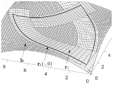
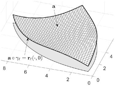
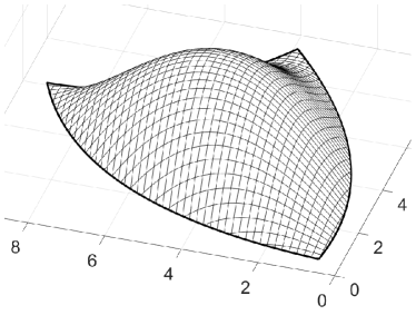
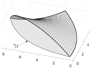
Let be a spline surface, called base, and be a sequence of other spline surfaces, called ribbons. Then we define the ABC-surface
with suitable reparametrizations and weight functions and . Figure 1 illustrates the setting. It is instructive, but not necessary, to think of as a standard spline surface describing the overall shape to be designed. When trimmed, its boundaries are close to the desired behavior, but do not match exactly. The ribbons are employed to adjust that deviation.
The domain of is assumed to be bounded by smooth segments meeting at corners . The base describes the intended shape globally on , and each ribbon describes that shape locally in a vicinity of the segment of the boundary. This is done in such a way that the spline curve parametrizes the segment of the boundary of the trace of . The reparametrizations are used to reconcile the otherwise unrelated surface representations, and the weights are used for blending. When approaching the boundary, vanishes and makes the base disappear. Further, near the boundary segment corresponding to all weights except for vanish so that also all ribbons but are faded out. Hence, this surface dominates the behavior of near the boundary in a way that will be made precise below. The accurate boundary control of the surface by means of ribbons explains the acronym ABC-surface.
The basic principle and some technical details of ABC-surfaces were first presented in [Rei]. Roughly at the same time and independent of our research, another group developed similar ideas [VVSS20], which were recently brought to our attention. The formal similarities are obvious, but there are also differences, and one of them is significant.
First, the weighted base does not appear in that form555It does appear in a similar form in [VSR12] for the special case of straight boundaries and polynomial ribbons. in [VVSS20]. Instead, a linear combination of control points and B-splines is used, where only B-splines with support completely contained in the domain of the surface are permitted so that there is no influence on the shape near the boundary. Accordingly, the term in the denominator is replaced by . This can be considered a minor technical detail, but it also reveals a slightly different, though equally valid philosophy behind the construction. We think of the base as a relatively accurate description of the entire surface, and of the ribbons as small, local correctives, used only to adapt to the desired boundary behavior. By contrast, the ribbons in [VVSS20] are the major building blocks for the shape to be modeled. The summands , if included at all, are only used for variations inside if the shape defined by the ribbons alone does not yet meet expectations.
Second, and this difference is much more important, the surfaces constructed in [VSVS20, VVSS20] are transfinite in the sense that they do not possess a closed-form representation by means of elementary functions. In particular, these surfaces are not piecewise polynomial or rational and thus cannot be stored in standard file formats, as requested in many applications. The point is that the curves bounding the domain are defined explicitly as splines. Once this is done, there is no way to continue the construction within the spline framework. For instance, it is in general impossible to find splines that vanish on all but one of these boundary curves666 The special case of straight boundaries, which admits rational constructions, was discussed in [VSR12, SVR14, VSK16, VSK17].. In [VSVS20, VVSS20], it is suggested to construct reparametrizations and weights as solutions of variational problems with the curves providing the boundary conditions. This requests a certain computational effort, but visually, the results appear to be excellent. By contrast, in our construction, the boundary curves are defined implicitly as zero levelsets of spline functions. That way, the problem described above disappears. It may be objected that explicit evaluation of the boundary of the domain is now much more expensive than it was before, but as a matter of fact, this is hardly ever requested in practice as long as the spatial boundary curves are available.
The paper is organized as follows: In the next section, we introduce and analyze the basic principle for the construction of ABC-surfaces in a very general setting. Three theorems concerning the behavior of positions, normals, and curvature tensors at the boundary are provided. They establish the validity of our construction, but also that of the methods presented in the more application-oriented papers [SVR14, VSVS20, VVSS20]. In Section 3, we specialize the principle to the spline setting and describe in detail how to construct adequate reparametrizations and weights from given bases and ribbons. Section 4 addresses some important technical issues related to the limitations of current standard formats for file exchange with respect to trimming. Finally, in Section 5, we present a few examples of ABC-spline surfaces to demonstrate the potential of our method.
2 Basic principle
Throughout, boldface letters denote points and functions with values in , while greek letters denote points and functions with values in . Except for the surface to be constructed, all functions appearing below are assumed to be sufficiently smooth. In particular, their derivatives mentioned anywhere (explicitly or implicitly through notions like normals or curvatures) are assumed to exist and to be continuous. Further, to avoid a discussion of degenerate cases, surfaces are always assumed to be immersed, i.e., the partial derivatives are linearly independent everywhere. The following definitions are crucial for the construction of ABC-surfaces:
Definition 2.1
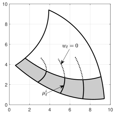
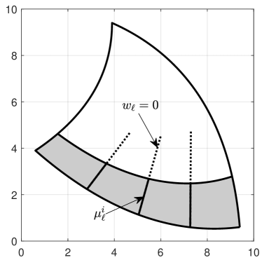
Now, we describe the construction of a surface , whose domain of definition is bounded by a sequence of planar trimming curves . When concatenated according to
| (1) |
these curves form a closed loop without self-intersections. Here and below, the index always runs from through and is understood modulo . Let
denote the corners and boundary segments of , respectively. Formally, the endpoint is missing in the definition of to obtain a disjoint union for the boundary of . Accordingly, for each boundary point , there exist unique values and such .
The building blocks for the construction of the surface are the following:
-
•
Let be functions that define trimming curves in the sense of Definition 2.1 according to the setting described above.
-
•
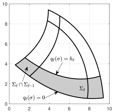
Let be an implicit representation of all trimming curves. That is,
Further, it is assumed that is positive on the interior of , see Figure 3 (left).
-
•
For each , let be an implicit representation of all trimming curves but . That is,
Further, it is assumed that is non-negative on , and that the only zeros of the sum in are the corners, see Figure 3 (right).
-
•
Let be a surface, called the base. Unit normal and curvature tensor of are denoted by and , respectively.
-
•
For , let be surfaces, called ribbons. Unit normal and curvature tensor of are denoted by and , respectively.
With these ingredients, we construct a new surface that combines base and ribbons in a specific way:
Definition 2.2
The ABC-surface corresponding to the data , as defined above, is given by
| (2) |
At corners, where the right hand side is not yet well defined, let
For the sake of simplicity, this definition is restricted to the case that the domain is simply connected and has always corners and boundary segments. Generalizations to multiply-connected domains and to disc-like surfaces bounded by one smooth, periodic curve will be discussed in a forthcoming report.
Two basic elements characterize the construction in the definition above. First, the functions , which define the trimming curves, are used as reparametrizations for the ribbons to adapt them to the otherwise unrelated base . Second, near the boundary segment the various implicit representations and are used as weights to fade out the influence of the base and all ribbons except for . The ribbon becomes dominant and determines the shape of . Thus, the construction provides accurate boundary control for , giving rise to the acronym ABC-surface. For a more detailed assessment of this raw idea, we need a further definition:
Definition 2.3
Let be an ABC-surface according to Definition 2.2. It has contact order at the boundary segment if for any it holds
and, unless or and , also
Further introducing the notation
for the reparametrized ribbons, can be written in the form
| (3) |
Here and below, the variable is always assumed to be fixed and mostly omitted in the notation for the sake of simplicity. Unit normal and curvature tensor of coincide with the respective quantities of since these surfaces are related by reparametrization,
| (4) |
In the interior of , is a blend of smooth surfaces and thus can be expected to be smooth, too. As always, exceptions may occur in case of an incidental loss of regularity. We will not discuss such degenerate cases, but focus on the behavior of at the boundary. The following three theorems clarify the situation:
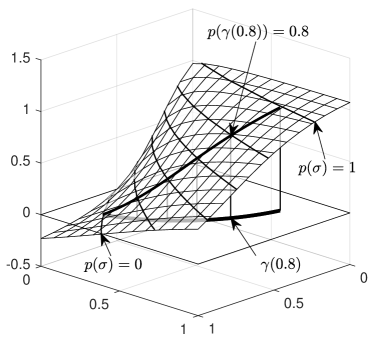
Theorem 2.4 (-boundary)
Consider an ABC-surface according to Definition 2.2 with contact order at . If the ribbons are consistent according to
then is continuous at , and it holds
| (5) |
In the following proofs, it is convenient to use the abbreviations
to expand in a vicinity of the corner . Since weights are assumed to be nonnegative, it is . For contact order , we obtain
| (6) |
Proof. Consider the point and in the form (3). We note that and, by consistency, . For , (5) follows from
For , (6) yields
In the following, denote the partial derivatives of the bivariate function , respectively. denotes the Jacobian.
Theorem 2.5 (-boundary)
Proof. Analogous to the previous proof, we obtain for
Differing only by second order terms, the surfaces and have the same normal at the origin. Hence, using (4), we obtain
Below, we mostly omit not only notating , but also the argument . For , corresponding to the case , (6) yields the derivative
By consistency of ribbons, it is so that
Let us consider the leading matrix, defined by the first two summands. Since , it is a convex combination of and . By the regularity condition, it has rank , and by consistency of normal vectors, both columns are perpendicular to . Hence, normalizing the cross product of these columns and passing to the limit yields , as stated. Clearly, in general, the derivative itself does not possess a limit for .
We note that the regularity condition (7) is purely technical and typically satisfied. It rules out a degenerate situation, which can occur in a similar way anywhere in any common surface modeling system for an unfortune choice of control data.
The crucial conditions for the existence of normal vectors at the boundary are algebraic (proper decay of the functions and ) and geometric (consistency of ribbons and normals). Similar conditions appear in the following theorem concerning curvature tensors. However, and this may be unexpected, also a parametric condition (consistency of derivatives of ribbons) has to be met to guarantee existence of a curvature tensor at corners.
Theorem 2.6 (-boundary)
Proof. As before, we obtain for
Differing only by third order terms, the surfaces and have the same curvature tensor at the origin. Hence, using (4), we obtain
Analogous to the previous proof, we obtain for , corresponding to the case ,
and, using (9),
This time, the derivative has a limit at the corner,
| (11) |
The second order partial derivatives are given by
where we used that and . Further, the curvature tensors of and coincide at the origin, . This implies that also the second fundamental forms coincide,
The second fundamental form of is
By Theorem 2.5, the normal vector of converges, i.e., . Hence, we obtain
and finally, using ,
Together with (11) and (4), this implies coincidence of curvature tensors,
and the proof is complete.
The proofs of the three theorems show that -properties on the interior part of the boundary segments are easily achieved by requesting proper decay of the functions and . Consistency and regularity conditions are requested only to guarantee good behavior at the corners. Remarkably, condition (9) concerning consistency of the derivatives of reparametrized ribbons shows that the functions cannot be chosen independently of the ribbons . More precisely, the interrelation
| (12) |
must be observed. Assuming that the ribbons are given and the reparametrizations are still unknown, this equation yields a linear constraint on the pair at the corner . Vice versa, if the reparametrizations are given, the space of admissible ribbons is restricted to a linear subspace.
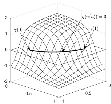
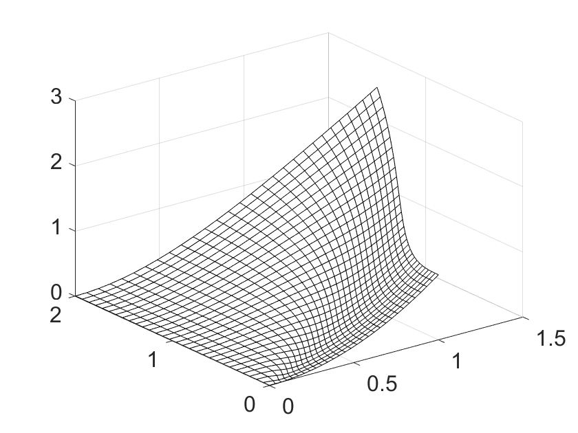
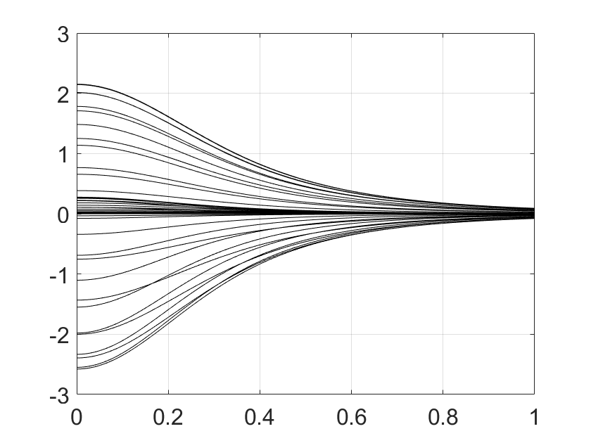
The following example shows that this condition is in fact crucial. Let
Near the origin, the traces of both surfaces coincide so that consistency of point, normal, and curvature tensor is guaranteed. However,
The weight functions have proper decay at the boundary curves and . Assuming for simplicity that the base and all other ribbons vanish, we obtain
Skipping the technical details, we note that
and
However, the curvature tensor is discontinuous at the origin. Figure 4 shows the surface (left) and the Gaussian curvature (right) as a function of . The individual lines correspond to equally spaced angles in the interval . For and , corresponding to the trimming curves and , it is , as suggested by the cylindrical shape of and . However, other angles yield non-zero limits.
3 ABC-spline surfaces
In the previous section, the ABC-principle was introduced in great generality. Our main goal, however, is to find a special embodiment of the setup that is fully compatible with the predominant standard of industrial surface modeling: trimmed NURBS.
To this end, we assume that all building blocks of the ABC-surface are tensor product NURBS. Even more, for the sake of simplicity, we consider only purely polynomial, i.e., non-rational splines. Further, it is practical (but not necessary) to use a common set of knot vectors for the base , the weights and the reparametrizations ; degrees may be different. By contrast, the knots of the ribbons are completely independent. It is immediately clear that the concatenation, multiplication, summation and division of piecewise polynomial functions yields a piecewise rational function . Denoting the coordinate degree of the bivariate spline by and its total degree by , we obtain
Together, the maximal degree of the rational pieces of equals that of the corresponding numerators, and is given by
| (13) |
where the maximum is taken component-wise. More specific results will be presented later on.
The crucial question that has to be addressed now concerns the construction of suitable splines , and . In recent works [VSVS20, VVSS20], reparametrizations for domains bounded by curves are obtained as solutions to variational problems with the given trimming curves as boundary conditions. It can be expected that this yields good visual results, but of course, there does not exist a closed-form solution, and much less a spline fulfilling the condition . Similar problems arise when seeking weights vanishing at the boundary or parts thereof.
The solution of the problem to find weights and reparametrizations compatible with the boundary is amazingly simple: There is no need to define the boundary curves explicitly. It suffices to define them implicitly by the functions according to Definition 2.1,
This setting is justified by the fact that standard CAD systems and also standard file exchange formats like STEP or IGES allow trimming curves to be specified explicitly as a closed loop of spline curves in the parametric domain, or alternatively–and this is the option used here–as a closed loop of spline curves in bounding the trace of the given NURBS surface. By Theorem 2.4, the curves
can serve exactly that purpose. Actually, the planar trimming curves need not be computed at any processing step of ABC-spline surfaces as long as geometric trimming by spatial curves, as explaind in Section 4, is available.
Now, we elaborate on methods how to determine suitable reparametrizations and weights under the assumption that the base and the ribbons are given.
3.1 Reparametrization
In principle, the functions can be chosen quite arbitrarily. Basically, only the consistency condition (1) must be satisfied. This means that there exist points such that
for all . If continuity of curvature tensors is requested, also condition (12) must be observed, i.e.,
| (14) |
Further, to obtain fair surfaces, it is reasonable to request that reparametrizes in such a way that it is close to the base,
The simplest way to achieve this (and possibly other desirable properties) is as follows: First, for each , we consider pairs of parameters , characterized by
Collecting a sufficiently large, but finite number of them yields the set . Such pairs can be found easily by requesting that the line connecting the points and be perpendicular to one of the two surfaces. To address the special role of corners, the set must contain the values and . The corresponding -values must be consistent in the sense that the corners
are well-defined. At this and possibly other data points, the function should not only approximate but interpolate the prescribed values. More precisely, let be the subsets of pairs intended for interpolation and the remainders. In particular, the pairs and addressing the corners belong to . Now, the conditions to be satisfied by are
Standard techniques, including all kinds of least squares methods or smoothing splines can be used to select accordingly from a given space of splines. If the problem is overconstrained in the sense that no solution exists, the spline space must be enlarged or the conditions must be relaxed. Conversely, if the solution is not unique, the spline space must be reduced or more conditions must be specified.
The interpolation conditions and for the corners yield
as requested by (1). Still, condition (14) needs to be addressed. When needed, one determines matrices such that
In particular, the columns of span the wanted tangent space at . Now, is determined as before, but such that is satisfies the additional conditions
As the chain rule shows, this is in accordance with , and it also implies (14).
3.2 Weights
Once the reparametrizations are known, also suitable weights and can be determined conveniently.
By definition, the second coordinate of vanishes at . Assuming that the ABC-surface to be determined should have contact order at the boundary segment , the simplest choice for is
| (15) |
where the exponents are . At this point, it has to be made sure that each factor is positive on . Additional zeros away from are not critical. Increasing some control points of B-splines vanishing at that boundary segment, these zeros can be removed without changing the crucial boundary behavior. However, zeros near the boundary may be persistent so that the whole construction fails. In particular, reentrant corners are likely to cause such a situation. This case requires a special treatment and will be discussed in a forthcoming report.
Omitting one factor yields possible weights
Let us check the conditions concerning contact order given in Definition 2.3. For , we obtain
since . Further,
unless the denominator vanishes at , and this is only possible if or and . Exactly these cases are excluded in the definition.
The weights suggested above have two drawbacks: First, the influence of each ribbon extends over the whole surface, which might be unwanted. Second, the polynomial degree of such weights is increasing with . If, for example, , , and for all to achieve contact order everywhere, then . This might cause problems with efficiency of storage and speed of evaluation after converting the surface from its procedural definition (2) to the usual form
of a NURBS surface, i.e., the linear combination of control points by means of B-splines and (constant) weights . The latter is requested in particular for the export of to standard file formats, as addressed in the next section. The following modification of weights away from the boundary of the domain solves both issues:
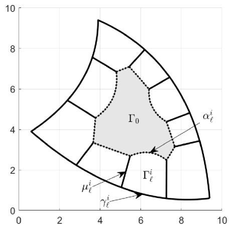
Denote by
the boundary stripes of with width . The widths are assumed to be chosen small enough to make sure that only boundary stripes of neighboring curves intersect, and that these intersections as well as the stripes themselves consist of a single connected piece, see Figure 5 (left). Now, we derive from a new spline as follows: First, classify the indices in the B-spline representation according to
That is, B-splines affect the boundary if , and they affect the part beyond the boundary stripe if . Second, if the sets and are not disjoint, refine the B-spline representation of by knot insertion and repeat the first step. Third, set
| (16) |
Coefficients with indices neither in nor in are determined such that the resulting spline has reasonable shape, for instance by minimizing a standard fairness functional. Fourth, define the spline . By construction, is an implicit representation of , but has a plateau with constant value beyond the boundary stripe . Figure 5 (right) illustrates the procedure exemplarily in the univariate case. Replacing (15) by
we obtain an implicit representation of with plateau on the interior part of the domain that is not covered by a boundary stripe, see Figure 6 (left). By construction, the coordinate degree of is bounded by
since at any given point at most two factors are non-constant. Notably, the degree does not depend on the number of boundary segments. In the example above, we have now . This is still a relatively high degree, but much less than before, and can be considered manageable.
The weights may be modified in a similar spirit. We define the functions
and process them exactly like the functions above, but now replacing (16) by
This way, we produce a function with a zero plateau beyond the boundary stripe. The desired weight is now simply given by
see Figure 6 (right). The degree
is again independent of .
Let us reconsider the degree of for weights and with plateau, as defined above. For simplicity, we assume that and , and that all contact orders are equal to . Then, using (13),
The coordinate degree of the ribbons is set to the unmatched pair for the following reason: In the first direction, corresponding to the behavior along the boundary, full flexibility concerning the choice of knots and degrees is provided to model a large variety of shapes. By contrast, in the second direction, corresponding to the behavior transversal to the boundary, it is sufficient to deal with pure polynomials of low degree. For instance, choosing allows the definition of the boundary curves and the boundary normals along . When also the curvature tensors shall be prescribed, it suffices to choose . The minimal configuration yielding a -patch and contact order requests and , leading to . For a -patch and contact order , one chooses at least and to obtain .
Modeling with surfaces of such a high degree is commonly considered to be impractical. However, this is never requested. The geometric building blocks–base and ribbons–can be assumed to be splines of low degree, and their control points can be manipulated (manually or automatically) as usual. The conversion of the ABC-surface to NURBS form
as detailed in the next section, serves only the purpose to prepare it for file export according to industrial standards. It should be considered as a read-only representation, to be used for evaluation purposes. Never ever, the control points should be touched again after being derived from (2).
4 File export
As a matter of fact, data exchange between industrial CAD/CAM systems is limited to a few completely standardized file formats, like IGES or STEP. The only type of surfaces commonly available therein are trimmed NURBS. Other modeling paradigms, say based on box splines, exponential splines, or subdivision are typically not supported. For the trimming of a NURBS surface , the following three options can be assumed to be available:
Parametric trimming. A closed loop of planar spline curves without self-intersections is specified. The compact set bounded by these curves is used as the domain of the trimmed surface .
Geometric trimming. A closed loop of spatial spline curves is specified. Since it cannot be assumed that the traces of these curves are contained in the surface, the corresponding planar curves are defined by where is chosen such that with the help of some projection method. These curves need not be splines by themselves, but are computed numerically. They are merely assumed to form a closed loop, which is bounding the domain .
Hybrid trimming. Some segments of the boundary are defined by planar spline curves, and the other ones by spatial spline curves. The planar curves together with the preimages of the projected spatial curves are assumed to form a closed loop, which is bounding the domain .
As we have seen, ABC-spline surfaces are piecewise rational. But nevertheless, in general, they cannot be represented as trimmed NURBS in the requested way. The point is that the summands may produce inner boundaries between rational segments that are not axis-aligned in the parameter domain and hence cannot be understood as knot lines. To solve this issue, we present a special construction of the reparametrizations that leads to a situation where can be represented as the union of separate parts, each of which is a genuine trimmed NURBS surface with boundary segments given either geometrically by a 3d spline curve or parametrically by a 2d spline curve.
For a spline of degree with knot vector , the natural domain of definition is the interval . We assume that can be evaluated on all of by simply prolonging the leftmost polynomial piece from to and the rightmost piece from to . Hence, true break points, where higher order derivatives are discontinuous, appear only at the inner knots .
Denote the knot vectors of by . We start with considering the second vector . Critical points that are mapped to the knot line for some inner knot by the reparametrization are characterized by
In general, neither the levelsets of nor their images under are splines. Special constructions for to create such a situation are possible, but impractical. It is much easier and completely sufficient to request that does not possess any inner knots at all. For instance, we may assume , what is just the knot vector for polynomials in Bézier form. We identified this setting already at the end of the preceding section as a legitimate choice. To sum up, ribbons that are pure polynomials in the second coordinate are able to carry information on location, unit normal, and curvature tensor along the boundary curve, and they do not have breaks in the second coordinate.
The treatment of the first variable is more involved since assuming also this dependence to be purely polynomial would unduly restrict the variety of shapes that can be modeled. Critical points that are mapped to the inner knot by are characterized by
This time, it is appropriate to demand that the critical levelsets of corresponding to inner knots of are linear. More precisely, let
denote the relevant parts of the levelsets of corresponding to the knots . In general, these curves are bent, see Figure 7 (left), but can be determined such that they become straight lines, see Figure 7 (right). One may proceed as follows:
First, for each knot , choose a direction such that
for arguments within the boundary stripe . Denoting by the pseudo-inverse of the Jacobian , one may set in particular
Second, define the line segment
with direction within the boundary stripe . Third, choose sufficiently many pairs of points of the form
and add them to the set of data to be interpolated.
Using this setup, points that are mapped to the inner knot of by either lie on the straight line or are irrelevant since .
Assuming that the ribbons are polynomials in the second variable and that the level sets are straight, as described, we can partition the domain into an interior part and boundary parts by a network of curves, consisting of three different types: First, there are the segments of the trimming curves corresponding to intervals between consecutive knots in . Second, there are the level sets , and third, there are auxiliary spline curves , to be chosen at will, connecting the endpoints of the level sets. Figure 8 illustrates the setting. Restricting the ABC-surface to the subdomains yields pieces , respectively, which are trimmed NURBS surfaces ready for filing with standard data formats. They do not have interior breaks aside from a regular knot grid, and their boundaries are formed by spatial spline curves and planar spline curves .
5 Examples
The focus of this article is on theory, but still, skipping many technical details, we want to present three examples to illustrate the potential of our approach. They show in turn composite surfaces with , and contact according to theorems 2.4, 2.5, and 2.6, respectively. All surfaces, reparametrizations, and weights are bicubic tensor product splines; all weights are used in the version with plateau.
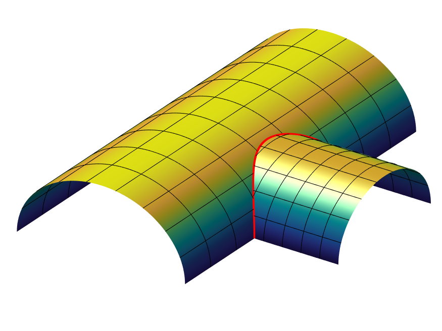

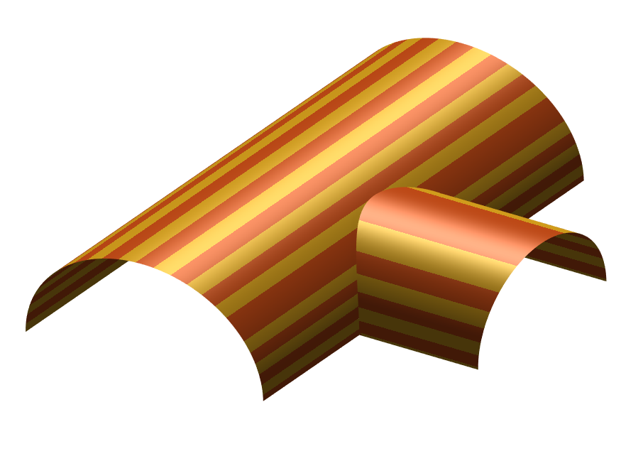
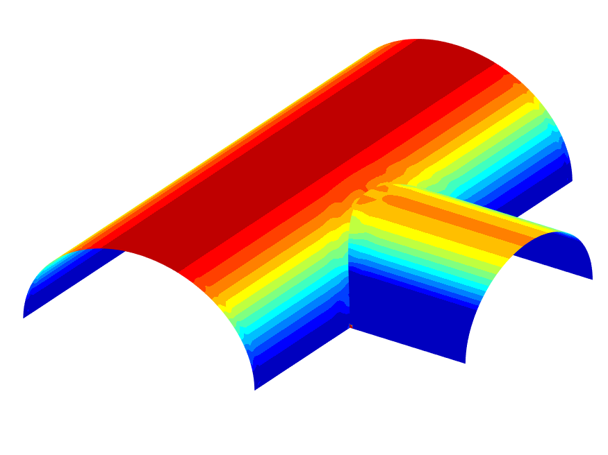
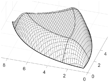
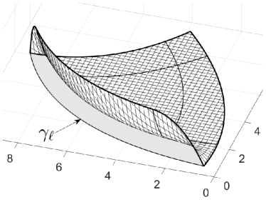
Figure 9 presents a typical example from solid modeling: two intersecting cylinders that trim each other. The first plot shows two ABC-surfaces together with a few parameter lines, which follow the given shapes in the natural way. The spline representations of the two original cylinders serve as bases for , respectively. The second plot shows the pair of ribbons used to model the region near the intersection curve. Both ribbons have interior knots in longitudinal direction. Their parametrizations are adapted to the local situation and chosen such that they share a common curve . This curve approximates the exact intersection of the two original cylinders with high accuracy. The watertight connection of ribbons is easy to achieve by coinciding boundary control points since both ribbons are in Bézier form in transversal direction. Theorem 2.4 says that this property is inherited by the two ABC-surfaces, i.e., they also join seemlessly at . The third plot shows the impeccable pattern of isophotes, while the fourth one is colored by mean curvature. Only here, one can see that the two surfaces slightly deviate from the perfect cylindrical shape of the original surfaces. This deviation could be made arbitrarily small by choosing finer knot sequences. However, as a matter of fact, it is impossible to do without any deviation since the exact intersection of the original cylinders cannot be represented by a spline curve–neither in geometry space nor in the parametric domain.
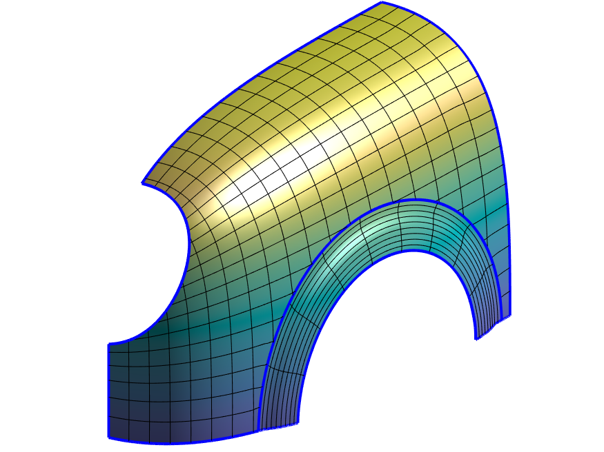
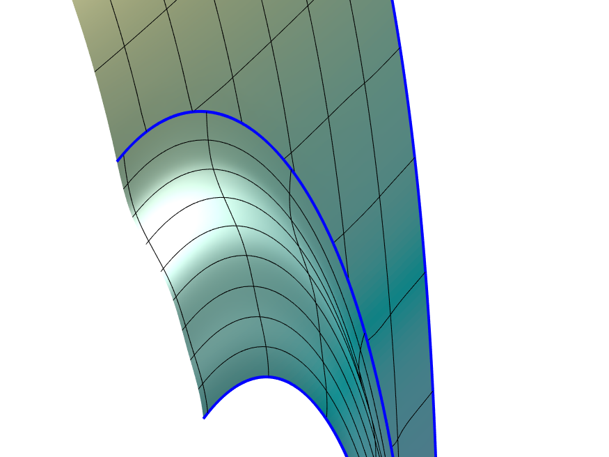
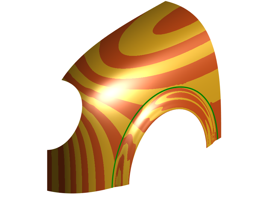
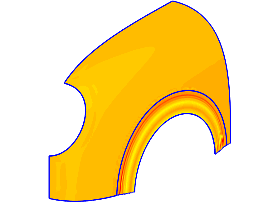
Figure 10 shows the fender of a fictional car777The geometry shown here was kindly provided my Malcolm Sabin, who modeled a similar composite -surface using a completely different, hitherto unpublished technique.. The whole geometry consists of a bigger, uniformly curved part and a bulged-out, annular area that can be viewed as part of the wheel case. While it is possible to model the object by a single spline surface, it is much more convenient and natural to assemble it from two pieces. The ring-shaped part is modelled by an untrimmed standard spline surface . The other part is an ABC-surface , whose ribbon along the junction has -contact with , which is easy to achieve. This implies coinciding normals along the common boundary, and hence, by Theorem 2.5, a contact between and . The first plot shows the complete composite surface, while the second one features a zoom on a cross-section profile. The third and fourth plot show isophotes (which are continuos) and mean curvature (which is discontinuous), respectively.
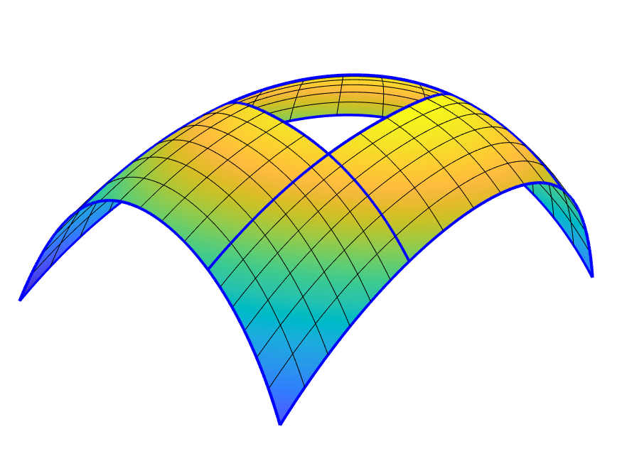
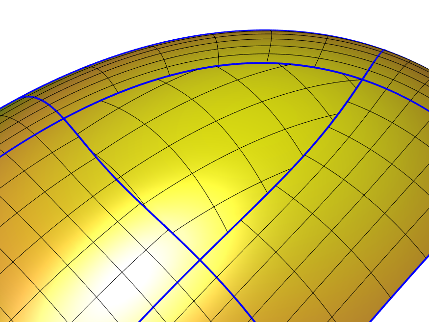
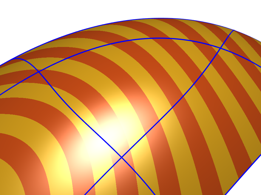
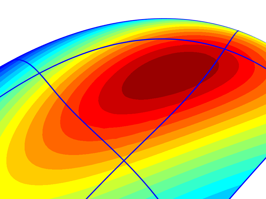
Figure 11 presents a classical hole-filling problem. Several standard spline surfaces are surrounding a triangular region, and another surface is sought that closes the gap smoothly. Here, we show that this can be achieved by an ABC-surface with three ribbons, each joining with the corresponding outer part. By Theorem 2.6, this guarantees a -contact. The first plot shows the configuration defining the three-sided hole, and the second one the completed structure together with a few parameter lines. Isophotes and also the distribution of mean curvature, as shown by the third and fourth plot, indicate that the generated shape leaves little room for improvement.
Acknowledgement. We would like to thank Malcolm Sabin for fruitful discussions and comments.
References
- [MH17] B. Marussig and Th.J.R. Hughes. A review of trimming in isogeometric analysis: Challenges, data exchange and simulation aspects. Archives of Computational Methods in Engineering, 25:1–69, 2017.
- [MR] B. Marussig and U. Reif. Surface patches with rounded corners. In preparation.
- [Pet02] J. Peters. Geometric continuity. In M.S. Kim G. Farin, J. Hoschek, editor, Handbook of Computer Aided Geometric Design, pages 193–227. 2002.
- [PGVACN06] N. Pla-Garcia, M. Vigo-Anglada, and J. Cotrina-Navau. N-sided patches with B-spline boundaries. Computers and Graphics, 30:959–970, 2006.
- [PR08] J. Peters and U. Reif. Subdivision surfaces, volume 3 of Series Geometry and Computing. 2008.
- [Rei] U. Reif. System and method for defining trimmed spline surfaces with accurate boundary control. Patent application EP19192703.7.
- [Rei97] U. Reif. A refinable space of smooth spline surfaces of arbitrary topological genus. Journal of Approximation Theory, 90:174–199, 1997.
- [SVR14] P. Salvi, T. Várady, and A.P. Rockwood. Ribbon-based transfinite surfaces. Computer Aided Geometric Design, 31(9):613 – 630, 2014.
- [VSK16] T. Várady, P. Salvi, and G. Karikó. A multi-sided Bézier patch with a simple control structure. Comput. Graph. Forum, 35:307–317, 2016.
- [VSK17] T. Várady, P. Salvi, and I. Kovács. Enhancement of a multi-sided Bézier surface representation. Comput. Aided Geom. Des., 55:69–83, 2017.
- [VSR12] T. Várady, P. Salvi, and A.P. Rockwood. Transfinite surface interpolation with interior control. Graph. Model., 74:311–320, 2012.
- [VSVS20] T. Várady, P. Salvi, M. Vaitkus, and A. Sipos. Multi-sided Bézier surfaces over curved, multi-connected domains. Computer Aided Geometric Design, 78:101828, 2020.
- [VVSS20] M. Vaitkus, T. Várady, P. Salvi, and A. Sipos. Multi-sided B-spline surfaces over curved, multi-connected domains, 2020. Unpublished manuscript.