Triggered star formation by shocks
Abstract
Star formation can be triggered by compression from shock waves. In this study, we investigated the interaction of hydrodynamic shocks with Bonnor-Ebert spheres using 3D hydrodynamical simulations with self-gravity. Our simulations that the cloud evolution depends on two parameters: the shock speed and initial cloud radius. The stronger shock can compress the cloud more efficiently, and the central region becomes gravitationally unstable, a shock triggers the cloud contraction. However, if it is strong, it shreds the cloud more violently and the cloud is destroyed. From simple theoretical considerations, we derived the condition of triggered gravitational collapse which with the simulation results. Introducing sink particles, we followed the further evolution after star formation. Since stronger shocks tend to shred the cloud material more efficiently, the stronger the shock is, the smaller the final (asymptotic) masses of stars formed (i.e., sink particles) become. In addition, the shock accelerates the cloud, promoting mixing of shock-accelerated gas. As a result, the separation between the sink particles and the shocked cloud center and their relative speed increase over time. We also investigated the effect of cloud turbulence on shock-cloud interaction. We that the cloud turbulence prevents rapid cloud contraction thus the turbulent cloud is destroyed more rapidly than the thermally-supported cloud. Therefore, the masses of stars formed become smaller. Our simulations can provide a general guide to the evolutionary process of dense cores and Bok globules impacted by shocks.
1 Introduction
1.1 Triggered star formation
Galactic star formation is classified two main processes. One is “spontaneous star formation,” in which the contraction of molecular clouds and subsequent star formation proceeds without any significant external disturbances. The other is “triggered star formation,” in which external factors promote the compression of molecular clouds, which induces star formation. The external compression is driven by shock waves generated by stellar winds, supernova explosions, cloud-cloud collision. For example, Elmegreen & Lada (1977) suggested that the compressed dense layer between shock and an ionization front can be gravitationally unstable. Cloud-cloud collisions have been proposed as an important mechanism in the formation of high-mass stars (e.g., Stolte et al., 2008; Furukawa et al., 2009; Wu et al., 2017). There is also observational evidence for star formation triggered by supernovae, ionization fronts, cloud-cloud and other shocks in the (e.g., Yokogawa et al., 2003; Ortega et al., 2004; Hester & Desch, 2005; Furukawa et al., 2009; Kinoshita et al., 2021).
, triggered star formation can occur when supersonic shocks sweep over clouds. The shock-cloud interaction is a fundamental and important physical phenomenon for star formation. , shock-cloud interactions are highly nonlinear hydrodynamic processes thus numerical simulation is tool to understand details. Over the past decades, the shock-cloud interaction has been explored by many groups (e.g., Klein et al., 1994; Xu & Stone, 1995; Boss, 1995; Nakamura et al., 2006; Pittard et al., 2009; Banda-Barragán et al., 2018). Most models assumed the two-dimensional (2D) axial-symmetric geometry. The first three-dimensional (3D) simulations were by Stone & Norman (1992). These simulations demonstrated that cloud destruction occurs faster in 3D the rapid growth of hydrodynamic instabilities in 3D. Later, the effects of various physical factors were explored by including turbulence (e.g.,Pittard et al., 2009), magnetic felds (e.g., Fragile et al., 2005), and radiative cooling (e.g., Mellema et al., 2002). incorporated self-gravity. These studies revealed the details of triggered star formation by shocks in the context of the formation of our System triggered by a supernova shock (e.g., Boss, 1995; Foster & Boss, 1996; Vanhala & Cameron, 1998; Vanhala & Boss, 2002 Boss et al., 2008; Leão et al., 2009; Boss & Keiser (2013); Li et al., 2014; Falle et al., 2017). These previous studies demonstrated that isothermal shocks can trigger gravitational collapse of stable clouds. Boss & Keiser (2013) that faster shocks destroy and disperse the cloud material before its collapse. , Falle et al. (2017) that slower shocks cannot induce collapse. These previous results indicate that only intermediate-speed shocks can trigger gravitational collapse.
Additionally, clouds and cores contain turbulent motions. Recently, Banda-Barragán et al. (2018) performed numerical experiments to investigate how cloud turbulence influences the shock-cloud evolution in the absence of self-gravity. They suggested that cloud turbulence cloud destruction and influences several ISM properties such as cloud porosity. Supersonic turbulence also enhances the acceleration of clouds to shocks.
In this , we 3D hydrodynamic numerical simulations to study shock-cloud . We an isothermal shock interacting with a Bonnor-Ebert sphere. In these simulations, self-gravity and sink particles included. This initial setup similar to those of Li et al. (2014) and Falle et al. (2017). Li et al. (2014) considered an application to the formation process of our Sun a shock-cloud interaction. Thus, their initial conditions very specific. Falle et al. (2017) investigated the early stages of shock-cloud and derived the condition for triggered collapse of stable Bonner-Ebert spheres. Here, we more general cases in a wider parameter range (from stable to unstable clouds). The inclusion of sink particles us to follow much longer evolution of the shock-cloud evolution. We also the effects of cloud turbulence on the shock-cloud interaction by including transonic cloud turbulence, which is often observed in the cloud cores in star-forming regions.
In the context of astronomical objects, we these simulations to represent the interaction of ISM shocks with dense cores and Bok globules in star-forming regions. Although the observed dense cores and Bok globules not in perfect equilibrium, some that the density structures of the dense cores and Bok globules in reasonable agreement with those of Bonner-Ebert spheres (e.g., Bacmann et al., 2000; Kandori et al., 2005; Alves et al., 2001). In some star-forming regions such as rho Oph and Orion A, the majority of the cores is likely to be pressure-confined (Maruta et al., 2010; Kirk et al., 2017). Therefore, our initial setup of the simulations is expected to represent reasonable conditions are in the ISM.
This paper is organized as follows. In Section 2, we describe the numerical methods, initial conditions, and simulation models which we in this . In Section 3, we present the numerical results. , we discuss interpretations of simulation results in Section 4. We derived a simple analytic condition for triggered gravitational collapse. Finally, we summarize our results and conclusion in Section 5.
2 Numerical Methods
2.1 Basic Equations and Numerical Code
In this , the simulations conducted using Enzo111http://enzo-project.org, adaptive mesh refinement (AMR) code (Bryan et al., 2014). We used Version 2.6 of the Enzo code in a 3D Cartesian coordinate system . We numerically the following hydrodynamic equations for mass, momentum and energy conservation:
| (1) | |||||
| (2) |
and
| (4) |
where is the density, is the velocity, is the pressure, is the internal energy, is the enthalpy, is the gravitational potential. We the ideal gas law:
| (5) |
determined by solving the following Poisson’s equation
| (6) |
where is the gravitational constant is the density of sink particles assigned onto the finest grids by using a second-order cloud-in-cell interpolation technique (Hockney & Eastwood, 1988). See Section 2.2.5 for the details of the sink particles.
We a mean molecular weight = 2.3, and set to 1.00001 for an approximate isothermal assumption. In this , we the purely hydrodynamic problem ignoring radiative cooling, heating, magnetic fields, and thermal conduction.
2.2 Initial conditions
2.2.1 Problem setup
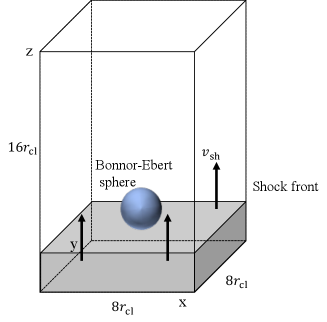
In the simulations, we the interaction between a planar shock and a Bonnor-Ebert sphere initially at equilibrium. Observations have indicated that the density profiles of dense cores and Bok Globules such as B68 can be approximated by that of a Bonner-Ebert sphere (e.g., Alves et al., 2001). Figure 1 shows the schematic of our simulation setup. The simulation domain a rectangular prism. The domain length of each side 8, 8, and 16, for , , and directions, respectively, where is the cloud radius. To follow the shock-cloud evolution, we set the side length in the z direction the shock propagates longer than the other two ( and ). The computational domain set to , , and . The initial Bonnor-Ebert sphere with a central density placed at the coordinate origin , and outside the cloud, we set the ISM gas with the constant density of . The density contrast of the cloud to the ambient gas at the cloud surface specified by
| (7) |
where is the cloud surface density. Initially, the cloud a temperature of and set in pressure equilibrium with the ambient gas, that is,
| (8) |
where is the cloud surface pressure, is the sound speed in the cloud, is the sound speed of the ambient gas. Therefore, the temperature of the external ISM .
We set an inflow condition on the bottom plane () in Figure 1 for a shock. For other boundaries, we an outflow boundary condition. the simulation , a planar isothermal shock to the positive z-direction toward the cloud through the ISM with a Mach number
| (9) |
where is the shock velocity.
Table 1 shows the initial simulation parameters. We set the cloud central density and temperature as and , respectively and fixed to , the ISM temperature K.
| \topruleParameter | unit | ||
|---|---|---|---|
| (K) | 10 | Cloud temperature. | |
| (K) | 103 | Preshocked amibient ISM temperature. | |
| (cm-3) | 104 | Central number density of the cloud. | |
| 102 | Density contrast between the cloud surface and the ambient ISM gas. | ||
| () | 0.19 | Sound speed in the cloud. | |
| () | 1.9 | Sound speed in the ambient gas. | |
| 2.0414.22 | Dimensionless radius of the cloud. | ||
| 1.207.00 | Mach number of the propagating shock. | ||
| 6.45 | Critical dimensionless radius (see Appendix A). |
-
•
Summary of the initial physical parameters.
2.2.2 Model Parameters
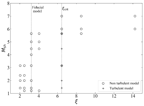
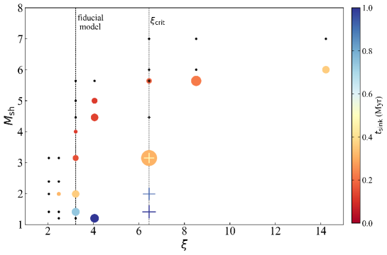
we . In this case, we shocks of = 1.20, 1.41, 3.15, 4.00, 4.46, 5.00, and 5.64. These Mach numbers correspond to postshock ambient gas pressure being , 2, 10, 16, 20, 25, and 32 times greater than those of preshocked gas. In addition to fiducial models, we considered a number of different simulation models with different dimensionless radii and shock Mach numbers, as summarized in Figure 2. Appendix 3 initial parameters of each model numerically. We both stable () and unstable initial clouds (). In stable clouds, we set = 2.04, 2.48, 3.22, 4.05 and 6.45. In our setting, to 0.034 pc (cf. Equation (A2)). These dimensionless radii to / = 0.125, 0.25, 0.5, 0.75, and 1.0, respectively. In cases, we = 8.52 and 14.22. These to = 28.08 (twice the density ratio of = 6.45) and 100.0, respectively. Although the initial cloud unstable in the cases, the free-fall time still longer than the shock arrival time and the cloud crushing time (see Appendix B.1). We discuss the cloud evolution triggered by shocks for cases.
2.2.3 Turbulent cloud models
In addition to the aforementioned models, we pure solenoidal turbulence to the fiducial Bonner-Ebert models where . A velocity power spectrum of added to the gas, where is the wavenumber. This power spectrum to the expected spectrum given by Larson’s law (Larson, 1981). The initial amplitude of the turbulence prescribed by the sonic Mach number
| (10) |
where is the velocity dispersion. In simulations, initially, we the clouds without shocks for 0.48 Myr to form the turbulent density structures in the clouds. , clouds with turbulent and velocity structures with shocks. The parameters of these turbulent clouds are indicated in Figure 2 (see also Table 3 , No.8).
2.2.4 Color variable
Similarly to previous simulations (e.g., Xu & Stone, 1995), to follow the evolution of shocked clouds quantitatively, we a Lagrangian tracer variable represented by
| (11) |
Initially, we for the cloud and for the ambient gas everywhere else. During the shock-cloud evolution, the cloud material with the ambient gas, resulting in regions with . We the variable to quantify cloud mixing rate as
| (12) |
where is the total mass in the zones with and is the cloud mass expressed as
| (13) |
Equation (11) describes the conservation law of .
We also the cloud living rate as
| (14) |
where is the total mass in the zones with .
To investigate the cloud motion, we the mass-weighted averaged cloud position in the z-direction defined by
| (15) |
2.2.5 AMR and sink particle condition
The simulation domain a top level root grid of with additional levels of AMR. We the following two criteria as the AMR condition to follow cloud evolution and collapse. In all models, the refinement until the finest resolution .
One AMR criterion based on . If the local region , one level AMR applied. this refinement, in all simulation models, the initial cloud radius divided into 64 cells. A resolution of 64 zones per cloud radius sufficient the shock-cloud evolution (e.g., Klein et al., 1994; Pittard & Parkin, 2016).
The other AMR criterion the Jeans criterion to prevent spurious numerical fragmentation. Truelove et al. (1997) that four cells per Jeans length are the minimum cells to prevent spurious numerical fragmentation. We the limit the Jeans length not fall below eight cells: , where is the Jeans length. In our simulations, the refinement until the density the threshold value , where is the initial cloud central density. That is, is as long as (see Equation (29) in Bryan et al., 2014). Applying the sound speed in the cloud and , . Therefore, in all models the refinement until . When the local density more than , instead of creating another AMR level, we the sink particle technique. this method, any excess mass in the cell above the transferred to the newly created point particle to avoid artificial fragmentation when the Jeans length further during the collapse. By that time it clear that the cloud collapse unstoppable. We set to (see Section 2.2.2) and is three or four orders of magnitude higher than the density of general molecular cloud cores. For , the isothermal approximation valid (for , the dense cores become adiabatic). , these particles through the grid gravitational interactions with the surrounding gas and other particles.
3 Numerical Results
Here, we will provide some numerical results. The clouds with =3.22 () stable initially. First, as a representative example, we will discuss cloud evolution using the results of =3.22 at different Mach numbers. In Appendix E, we other dimensionless radii cases. Finally, we will the results of turbulent cloud models.
In all cases, we tracked shock-cloud evolution until 10 of the initial cloud mass exited the simulation box.
3.1 Evolution of maximum density


|
The maximum density is a good indicator of cloud stability. Figure 3 shows the maximum density normalized to the initial central cloud density as functions of time after a shock at cloud. Hereafter, in all figures, indicates the time when the shock front first the surface of the cloud. The vertical dashed line one free fall time , where is the mean density of the initial cloud. The solid lines the cases for which gravitational collapse is triggered by the shocks. The cases the clouds not collapse after shock passage are dashed lines. Below, we these two cases “triggered-collapse case” and “no-collapse case” respectively.
One important feature is that only intermediate shocks of can trigger cloud contraction. For no-collapse cases, the maximum density at the beginning but to lower values after rebounding. For example, for the model with a weak shock of , the maximum density by one cloud free-fall time. However, it gradually with time. For the strong shock of , the maximum density at Myr. However, the maximum density to . Even for , the cloud once before collapsing at t = 0.43 Myr (point (1) in Figure 3). In triggered-collapse cases, the rate of density-increase becomes at the beginning. After some time, the rate of density-increase and the maximum density more than and sink particles are formed.
3.2 Density distribution
As in Section 3.1, the density evolution depends on the Mach number . Here, we present density distribution results for four cases: (1) a weak shock with =1.41, in which the cloud slowly collapses, (2) an intermediate shock with =3.15, in which the cloud rapidly collapses after shock passage, (3) a strong shock with =5.0, in which the cloud does not collapse, and (4) a weakest shock with =1.2, in which the cloud does not collapse.
3.2.1 Weak shock collapse (=1.41)
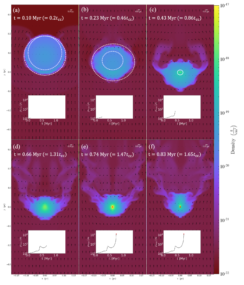
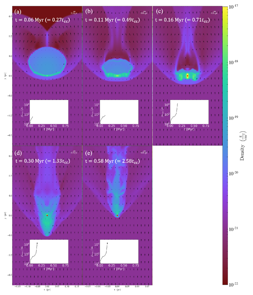
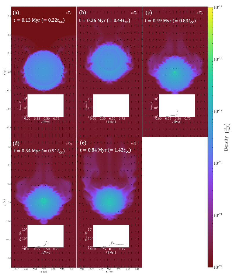
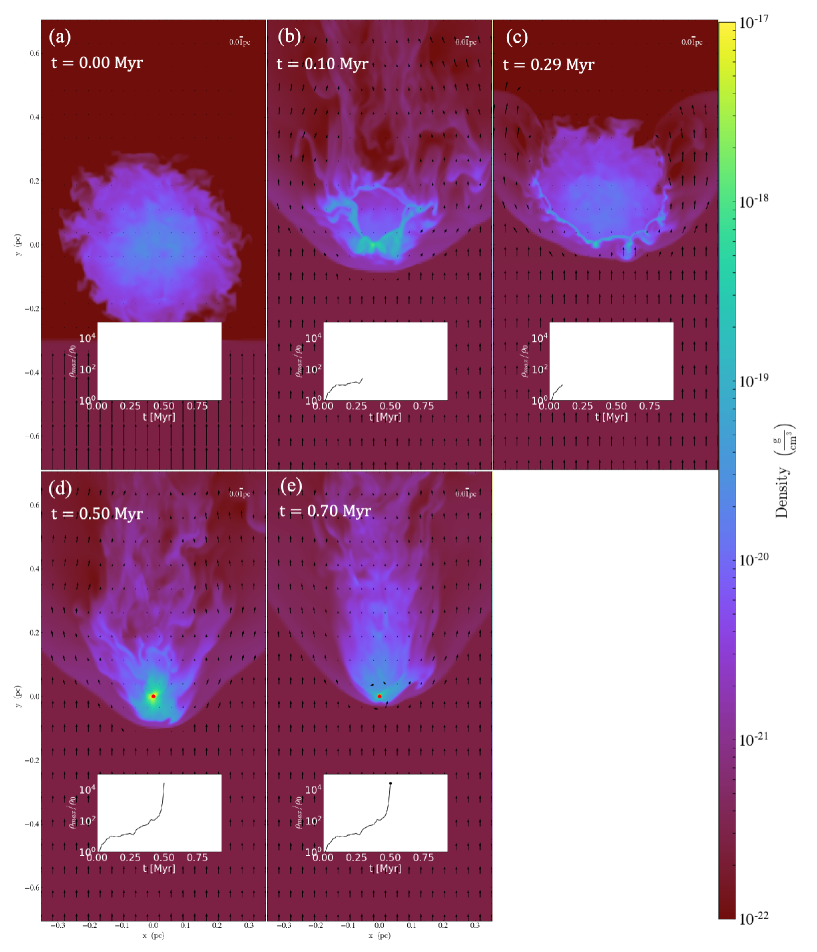
Figure 4 shows the time evolution of the mass density distribution in the plane for . In each panel, we the maximum density point. In addition to the times in Myr, the times in dimensionless units normalized to the cloud crushing time (see Appendix B) are also shown. We derived as . The time evolution of the maximum density are also shown in these panels. As Figure 4 (a) and (b) , the cloud surface compressed by the shock. The area surrounded by the white dotted lines indicates the compressed shocked layer formed by shocks propagating in the cloud. Myr, the shock propagating in the cloud from downstream with that from upstream, and the density at this collision (the area enclosed by the white circle in Figure 4 (c)). This phase to the maximum density rebounding (point (1) in Figure 3). After this rebounding, the higher density region not formed for a while. Myr, the cloud contracting again and the high density region formed again. As a result, a sink particle created at Myr. While the gas around the cloud center on the sink particle, as shown in Figure 4 (e), the gas at the cloud surface shredded gradually by the hydrodynamic instability.
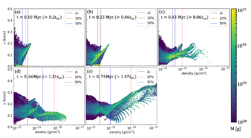
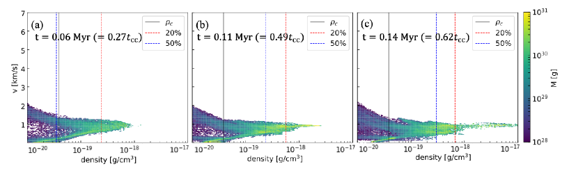
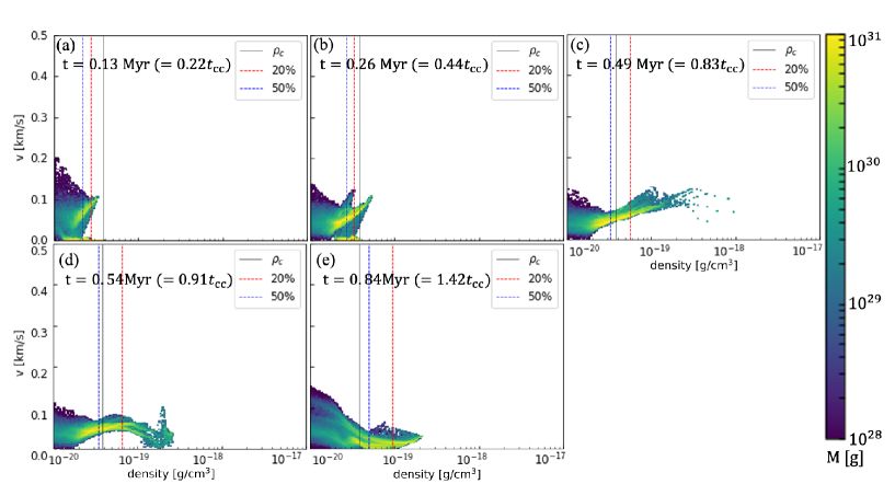
Figure 5 shows the . As shown in Figure 5 (a) and (b), shocks in the cloud, some shock-compressed gas accelerated and denser than the initial central density . Figure 5 (c) corresponds to the rebounding phase (point (1) in Figure 3). Figure 5 (d) corresponds to a density increasing phase when the maximum density the same value as Figure 5 (c) again (point (2) in Figure 3). Comparing the of Figures 5 (c) and (d), the mass fraction contained in the dense part to be larger for Figure 5 (d). By the time of Figure 5 (c), the cloud not contain sufficient mass to become gravitationally unstable. , by the time of Figure 5 (d), the central part of the shocked cloud more mass that the gravitational collapse initiated. After the rebound, the amount of dense gas as shown in Figure 5 (e), collapse.
3.2.2 Intermediate shock collapse (=3.15)
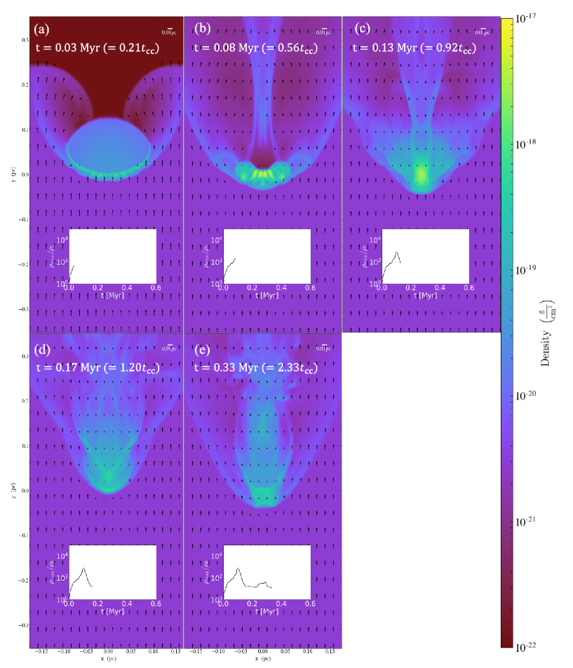
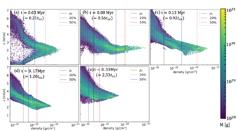
Figure 6 is the same as Figure 4 but for =3.15. As in the = 1.41 case, the cloud surface compressed by the shock and shocked layer to the cloud center. Unlike = 1.41, there no rebounding phase. A large high-density region formed, direct gravitational contraction and the creation of a sink particle t = 0.16 Myr. After the sink particle creation, the cloud around the particle stripped gradually. Eventually, it a comet-like structure with the sink as the head and the stripped gas as the tail. Figure 7 shows the similar to Figure 5. the shock in the cloud, high density gas developed monotonically, gravitational collapse.
3.2.3 Strong shock no-collapse (=5.00)
Figure 8 is the same as Figure 4 but for =5.00. As shown in Figure 8 (a) and (b), the cloud surface compressed by the shock, and the cloud but not collapse. After density rebounding Myr, the cloud destroyed and swept downstream of the shock mixing with the ambient gas.
Figure 9 shows the for =5.00. As shown in Figure 9 (a) and (b), high-density gas increased. Figure 9 (b) corresponds to density rebounding point for the =5.00 case (corresponding to the point (3) in Figure 3). After rebounding, evolution towards the high-density side stopped. Gradually, gas accelerated and distributed on the low-density side. This that the cloud accelerated by the shock, and cloud dispersed and at a higher speed downstream. In Figure 9 (b), the central denser cloud material velocity , and outer regions higher . While Figure 7 (c) (corresponding to (4) in Figure 3) has the same maximum density as Figure 9 (b), the cloud material lower velocity (). For =5.00, a high-density region initially formed, but the cloud accelerated more and dispersed before the gravitational collapse.
3.2.4 Weak shock no-collapse (=1.20)
Figure 10 is the same as Figure 4 but for =1.20. other cases, as shown in Figure 10 (a) and (b), the cloud surface compressed by the shock, and the compressed shocked layer to the cloud center. The maximum density t=0.49 Myr and gradually.
Figure 11 shows the for =1.20. Throughout simulation times, the high-density regions not as large as higher examples. Comparing Figure 11 (c) and Figure 7 (b), which have a common maximum density (points (5) and (6) in Figure 3), for Figure 11 (c), cloud mass has distribution on the high density side compared Figure 7 (b) =3.15. That is, = 1.20, a denser gas region not sufficiently formed compared the case of successful collapse. For =1.20, after rebounding, the surface of the cloud stripped toward the downstream shock.
3.3 Mixing and living rates
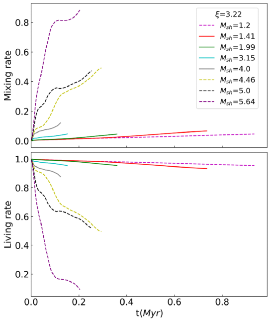
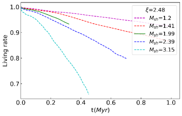
The top panel in Figure 12 shows the time evolution of the mixing rate defined in Equation (12). The larger the shock Mach number is, the faster the mixing rate . For = 4.465.64, at Myr when the maximum density rebound , the mixing rate , i.e. cloud gas mixed with the ambient gas. , for lower cases, the mixing rate not become higher than even when the cloud . A similar trend is indicated in the bottom panel in Figure 12, which shows the time evolution of living rate defined in Equation (14). For cases, rebounding, living rates 0.8, , for lower cases, living rates than 0.8 when maximum densities . During the cloud contraction, more gas removed in the larger cases than in the lower .
3.4 Evolution of sink particles
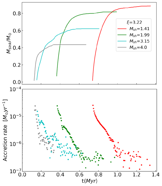
For triggered-collapse cases, the evolutions of mass and mass accretion rates of sink particles are shown in Figure 13. rates gradually by a few orders of magnitude and the mass of sink particles asymptotically. The top panel in Figure 13 indicates that the higher the Mach number , the lower the asymptotic sink particle mass . For =1.41, 1.99, 3.15, and 4.00, periods when mass accretion rates above , 0.22, 0.18, 0.13, and 0.07 Myr, respectively. The higher the Mach number , the shorter the time with high accretion rate . This trend of accretion timescale would affect the asymptotic sink particle mass.
3.5 Initially turbulent cloud cases
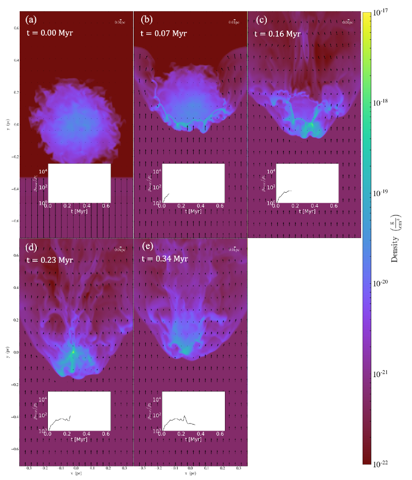
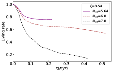
Here, we results of turbulent cloud models. We followed models of turbulent () clouds with a critical Bonnor-Ebert radius by changing the shock Mach number of . Figure 15 shows the time evolution of , , , , and accretion rates of sink particles. Figure 15 (a) indicates that shocks cloud collapse, relatively stronger and shocks not induce cloud collapse. Figure 16 and 17 show the slices of the mass density distribution for =3.15 and 4.46 as Figure 4. =3.15, a strongly compressed layer formed and then the cloud and . , =4.46, a strongly compressed layer formed initially the cloud later destroyed by the shock and mixed with the ambient gas. Figure 15 (b) and (c) indicate that the larger the Mach number , the shorter the mixing timescale with the ambient gas , higher living rates. Similar to the non-turbulent models, intermediate shocks cloud collapse, strong shocks destroyed clouds before collapse and mixed clouds with ambient gas faster. Figure 15 (d) and (e) show the evolution of mass and mass accretion rates of sink particles. Cross points in Figure 14 shows results of turbulent cloud models. The larger the Mach number, the shorter the span of effective accretion rate, and the lower the asymptotic mass of the sink particle.
 (a)
(a)
 (b)
(b)
|
 (c)
(c)
 (d)
(d)
|
 (e) Accretion rate of sink particles
|
To investigate the effect of cloud turbulence on shock-cloud evolution, here, we will compare turbulent models with corresponding non-turbulent models for the same cloud radius and shock Mach number. Figure 18 shows time of some physical quantities in both turbulent and non-turbulent models for and . Figure 18 (a) maximum density evolution . Up to Myr density evolution in two cases similar. , the turbulent cloud a slower increase in density. As shown in Appendix D, for the turbulent model, the sink particle was formed by 0.49 Myr after the shock touched the cloud, for the non-turbulent clouds model, it was formed by 0.31 Myr. That is, the turbulent cloud a slower increase in density and slower sink particle formation than the non-turbulent cloud. Figure 18 (b) and (c) show the evolution of mixing rates and living rates. For the turbulent cloud, the living rate faster and mixing rate faster than that of non-turbulent . That is, the turbulent cloud faster with the surrounding ambient gas and destroyed. Figure 18 (d) and (e) show the evolution of sink particle mass and accretion rates. The asymptotic sink particle mass in the turbulent cloud model lower than non-turbulent counterparts. The accretion rate by the turbulent cloud, this occurs at Myr for the non-turbulent . For the turbulent cloud, accretion time shorter and the asymptotic mass of the sink particle lower.
As above, the turbulence cloud contraction, the destruction of the cloud, and the mass of the formed stars. We can that turbulence in the dense cloud has the effect of suppressing star formation by shocks.
 (a)
(a)
 (b)
(b)
|
 (c)
(c)
 (d)
(d)
|
 (e) Accretion rate of sink particles
|
4 Discussion
4.1 Conditions for cloud collapse by shocks
 (a) , t = 0.16 Myr (=0.27 )
 (b) , t = 0.49 Myr (=0.83 )
|
 (c) , t = 0.06 Myr (=0.27 )
 (d) , t = 0.15 Myr (=0.67 )
|
 (e) , t = 0.03 Myr (=0.27 )
 (f) , t = 0.08 Myr (=0.56 )
|
As shown in Figure 14, shocks that are strong or weak cannot induce cloud collapse. This is because strong shocks tend to destroy the cloud hydrodynamic instabilities and weak shocks do not compress the cloud to become unstable. This implies the existence of parameter windows for cloud collapse. In this subsection, we the conditions for gravitational collapse triggered by shocks.
Figure 19 shows the for the models as Figure 5. The vertical axis shows the value of the velocity normalized by estimated propagating shock velocity at the cloud surface (see Equation (B1)). with the color variable in green, while those of were shown in red. The panels in the upper row are for the cases corresponding to and the rebounding phase. For , gas accounting for more than 50 of the mass compressed almost without being stripped. However, as mentioned in Section 3.2.4, the clouds not sufficiently compressed to develop gravitational instability. The panels in the middle row are for the cases corresponding to and before sink particle creation. In panel (c), the distribution is shaped like a horizontal V with the root at . The gas distributed from the root of V toward the origin of the figure corresponds to the gas compressed by the shock progressing to the center of the cloud. Gas distributed from the base of V to the upper left of the figure corresponds to gas stripped and dissipated by the shock. For , compressed gas dense, gravitational collapse. The panels in the lower row are for the cases corresponding to and the rebounding phase. In panel (e), the distribution is shaped like a V as in panel (c), but the V is wider and more gas is dissipated. As shown in Section 3.2.4, eventually, the entire cloud destroyed.
these results, two conditions must be for the cloud to contract. The first condition the degree of compression by shocks. For low , most of the gas does not become dense and gravitational collapse cannot be induced. It is assumed that for cloud collapse, compression to make Bonnor-Ebert spheres unstable is required. This condition would determine the lower limit of the Mach number. The second condition the destruction of clouds. Even if clouds are strongly , shocks with Mach numbers that the destruction of clouds. to collapse, the timescale for the development of gravitational instability must be shorter than that of destruction. This condition would determine the upper limit of the Mach number. Hereafter, based on the above two conditions, we will estimate the Mach number parameter window for the cloud collapse.
First, we consider the lower limit of . Considering an isothermal shock with a Mach number , the ambient gas pressure behind the shock is .
Considering conditions for a Bonnor-Ebert sphere to become unstable, we expect
| (16) |
where is the critical pressure of Bonnor-Ebert sphere (see Equation (A9)). This relation implies
| (17) |
Substituting Equation (A2),(A4) and (A6), we a dimensionless expression:
| (18) |
Since the side of Equation (18) is a function of , it can also be expressed a function of . the third degree polynomial regression of the side of Equation (18) in the range of , we the approximate equation of lower limit of
| (19) |
corresponds to . When , a Bonnor-Ebert sphere is unstable.
Next, we consider upper limit of . Iwasaki & Tsuribe (2008) that the timescale of the gravitational instability of isothermal layers bounded by shock wave with the Mach number is an order of where is the free-fall time scale of the preshock region. In our model, the sum of the timescale on which the shock propagates through the cloud and the timescale on which gravitational instability behind the shock is estimated
| (20) |
where is the free fall time scale of spherical cloud.
It is known that the timescale of the cloud destruction is the order of the cloud crushing time = (see Appendix B). Previous numerical hydrodynamical simulations that (e.g., Klein et al., 1994; Poludnenko et al., 2002). by shocks, gravitational instability must within the timescale of cloud destruction . Hence, we expect
| (21) |
This implies
| (22) |
This equation can be rewritten dimensionlessly as
| (23) |
the the minus third degree polynomial regression of the side of Equation (23) in the range of , we the approximate equation of upper limit of
| (24) |
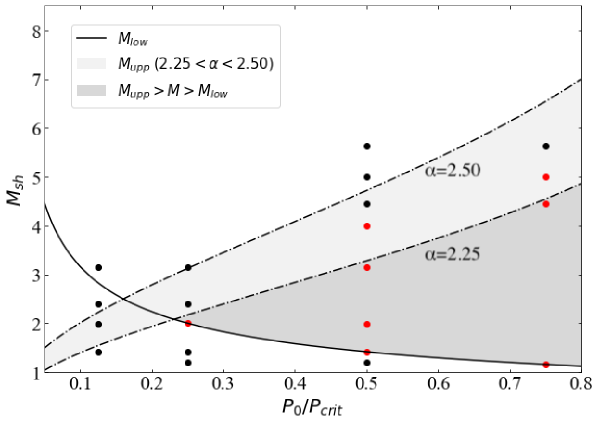
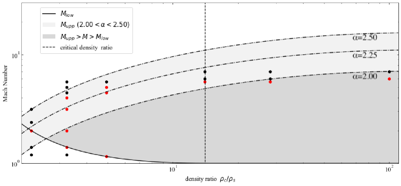
Figure 20 shows the pressure ratio vs parameter space for an initially stable Bonnor-Ebert sphere. The solid line demarcates the Mach number estimate based on Equation (18) above which the cloud will become unstable by the shock. The light gray shaded area shows the upper limit estimate for Mach number based on Equation (23) applying above which the cloud will be destroyed by hydrodynamic instabilities before the collapse. In the dark gray region, clouds are expected to be induced to collapse by shocks. Based on simulation results, red points indicate initial cloud parameter pairs corresponding to eventual collapse, while black points indicate cloud parameter pairs corresponding to predicted non-collapse. that red points are in dark or light gray regions and black points are outside of the light gray region. Hence, the simulation results are in agreement with our estimates of conditions. However, the upper limit estimate for Mach numbers has small range in terms of . This upper limit is derived based on estimate, and hydro instability is a complex process with uncertainty. It may be difficult to set an upper limit with a single line. the range of used is not large. The criteria we have derived are useful for estimates of stable cloud collapse.
Figure 21 shows the density ratio vs parameter space similar to Figure 20 with all parameter pairs shown in Figure 14. For initially unstable clouds (i.e. in the right-side region of the critical density line), when applying smaller ( 2.0), results of initially unstable clouds consist with the upper limit estimate. The reason for this gap in range between stable and unstable clouds is that for unstable clouds, the propagating shock speed estimated Equation (B1) and actual one an exact match. For unstable clouds, the density ratio is larger and a density gradient along the radial direction affects the shock velocity propagating in the cloud. Therefore, the timescale for shock propagation and cloud contraction expressed by the side of Equation (21) is affected, and the range changes. However, our upper limit estimate is useful for an order discussion. Although the upper limit has some uncertainty for larger unstable clouds, the general tendency of results is consistent with our estimate.
In our calculation, for clouds initially at , at the time when propagating shock to compress clouds, little gravitational collapse is in progress. That is, the density profile of the clouds is almost identical between the initial conditions and when the shocks arrive. We note that unstable clouds in which collapse has progressed further by the time the shock arrives, shock-cloud evolution may change and ranges of from our results.
4.2 Asymptotic mass of sink particles
 (a)
(a)
 (b)
(b)
|
As shown in Section 3.4, comparing results with the same initial radii, the higher Mach number of the shock is, the lower asymptotic sink particle mass and the shorter accretion time is. This would be because the higher the Mach number is, the faster the shock the cloud around sink particles. As shown in Figure 6, the cloud around the sink particle is stripped and mixed with ambient gas. Cloud material is accelerated and displacement of cloud material and the sink particle . , the accretion timescale would be determined by how the incoming shock can accelerate and strip accreting clouds from sink particles.
Here, we will the moving of stripped clouds and sink particles. We use the defined in Equation (15) to analyze the moving of stripped clouds.
Figure 22 shows the and position of sink particles in the z-direction for and . Displacement of the cloud and sink particle is initially small because of the low mass of sink particles. , the sink particle drifts behind and displacement becomes larger because accretion progresses and the sink particle mass .
 (a) Relative
 (b) Relative velocity
|
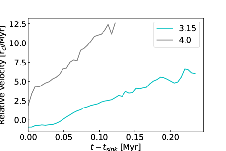
Figure 23 shows the relative and velocity and those of sink particles for and . The higher the Mach number of the shock is, the faster the relative and velocity . This trend is also for other radii (see Appendix F). Therefore, relative displacement and velocity of the particle and cloud determined by the shock speed and the timescale of accretion and asymptotic mass.
4.3 Effect of turbulence
Figure 24 shows the as Figure 19 for both turbulent and non-turbulent ( and ). Figure 24 (a) and (d) are at the same time. Figure 24 (b) and (e) also at the same time, and Figure 24 (e) corresponds to the before sink particle. Comparing Figure 24 (a) and (d), cloud mass less on the high density side compared . As in Section 3.5, the turbulent cloud has a slower increase in density and a slower sink particle formation than the non-turbulent cloud. This slowness would be due to the effective pressure from turbulence in the cloud. Internal turbulence increases effective cloud pressure to the order of . This increased pressure enhances cloud diffusivity and suppresses cloud contraction by the external ram pressure due to shock. Therefore, turbulence prevents rapid gravitational collapse and high density region is formed slowly.
Figure 24, throughout the evolution the turbulent cloud, the distribution of the gas shown in red () from that of the non-turbulent cloud. For example, in Figure 24 (d), red and green gas shows near V-shaped distribution, while in Figure 24 (a), red gas shows a fan-like distribution. In other words, more gas is dispersed and mixed with the ambient gas. This trend is consistent with that of Figure 18 (b) and (c). Clouds with a turbulent velocity are more prone to Kelvin-Helmholtz instabilities than non-turbulent counterparts. Therefore, that turbulent vortical motions in the clouds diffuse the cloud, and the timescale of the mixture becomes shorter.
Figure 23 shows the relative and velocity and those of sink particles for both turbulent and non-turbulent ( and ). For the turbulent case, throughout the entire evolution, the relative is greater than that of the non-turbulent case. Most of the time, the relative velocity is also greater for the turbulent case. One reason for this trend is that the cloud with a turbulent velocity is destroyed by the shocks and the gas around the sink particles is stripped faster downstream of the shock. Another reason is that, for the turbulent case, the sink particle formed later, and by the time mass accretion , more gas been accelerated. , the asymptotic sink particle mass in the turbulent clouds models is lower than the non-turbulent counterparts.
Comparing No.5 and No.8 models results in Appendix D, the upper limit of the Mach number for cloud collapse . In turbulent cloud cases, the upper limit of the Mach number is for the not turbulent cases, it is . , parameter window for the cloud collapse narrower for turbulent cloud cases.
, turbulence in the cloud makes triggered star formation by shocks more difficult. Pressure due to turbulence cloud contraction and facilitates mixing with the ambient gases. The asymptotic stellar mass . that our simulation models address magnetic fields. In a realistic ISM, magnetic fields exist and can alter the physical process of the shocked cloud. In this , we purely hydrodynamic cases and investigate the effects of turbulence.
 (a) Turbulent cloud model, t = 0.16 Myr
 (b) Turbulent cloud model, t = 0.31 Myr
 (c) Turbulent cloud model, t = 0.49 Myr
|
 (d) Fiducial cloud model, t = 0.16 Myr
 (e) Fiducial cloud model, t = 0.31 Myr
|
 (a) Relative
 (b) Relative velocity
|
4.4 Comparison with observation
4.4.1 Globules toward Orion’s veil bubble
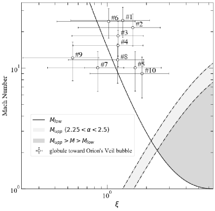
Extended Orion Nebula (M42) is photoionized by massive star in the Trapezium cluster, Ori C (e.g., O’Dell, 2001; Simón-Díaz et al., 2006). Using the IRAM 30m telescope, Goicoechea et al. (2020) and maps of “Veil bubble” by the strong wind emanating from Ori C. They the presence of ten CO “globules” blueshifted from the OMC and embedded in the expanding shell that encloses the bubble. These CO globules are small ( AU), not massive () and are moderately dense: (median values of the sample). Goicoechea et al. (2020) that they are either transient objects formed by hydrodynamic instabilities or pre-existing over-dense structures of the original molecular cloud. They are sculpted by the passing shock associated with the expanding shell and by UV radiation from the Trapezium. From the estimated masses of globules, deduced that these globules will not easily form stars. For some globules, their masses are greater than the Bonnor-Ebert mass (see Equation (A7)) less than Jeans mass.
We calculated dimensionless radii and of these globules assuming that they are ideal Bonner-Ebert spheres and pressure equilibrium with the ambient gas. We note that our calculations and estimation simplistic. In calculation, we magnetic fields and turbulence. We also the pre-shocked cloud sphere, but in these globules have been compressed to some extent. here is a to investigate the general trend. In our calculation, we adopted estimated globule parameters (, and ) listed in Table 1 in Goicoechea et al. (2020) and expanding shell speed =13 km s-1, assuming initial gas density between globules surface and surrounding ISM is 10. Figure 26 shows dimensionless radius versus Mach number parameter spaces. Derived parameter pairs of ten globules are plotted. As in Figure 20, estimated upper and lower limit of for collapse are also shown. Some globules are distributed in the parameter space above the , while all cores are distributed in the parameter space above the . That is, most globules are strongly compressed and become dense, but they are destroyed by shocks and star formation activities are limited. This prediction for the future star formation of these globules is consistent with the prediction by Goicoechea et al. (2020).
| \topruleglobule a | b | c |
|---|---|---|
| #1 | 1.320.79 | 24.96.99 |
| #2 | 1.570.98 | 21.76.51 |
| #3 | 1.210.68 | 18.55.88 |
| #4 | 1.210.66 | 15.45.14 |
| #5 | 1.630.96 | 10.13.64 |
| #6 | 1.030.61 | 24.46.73 |
| #7 | 0.850.50 | 10.13.65 |
| #8 | 1.200.70 | 11.74.18 |
| #9 | 0.540.32 | 12.24.32 |
| #10 | 1.851.11 | 9.0 3.33 |
-
•
a Corresponding to Table 1 in Goicoechea et al. (2020).
b Estimated dimensionless radius.
c Estimated Mach numbers of the propagating shock.
4.4.2 Mass surface density PDFs
Figure 27 shows time evolution of column -PDFs for and for . These are the distribution of the column density when looking at the box data centered on the initial cloud from the x-axis direction. corresponds to the triggered collapse case, while and correspond no-collapse cases. Although a sink particle is formed for , only gas is included in this figure.
For , until PDFs a broadening distribution, with rebounding . The distribution not and is not as broad as the other two PDFs. For , until PDFs a broadening of distribution. The foot of high-density side increases to . After the sink particle creation at , PDFs rebound. , the distribution also wider and foot of high-density side above . Compared the other two PDFs, the value of the vertical axis is generally smaller and the total amount of gas above is smaller. After , the distribution rebounds.
Depending on Mach numbers, each PDF different characteristics. However, since PDFs evolve over time, it is difficult to distinguish the presence or absence of collapse from only the -PDFs. The distribution tail to the high-density side does not necessarily triggered collapse, and PDFs of observational data .
 (a) ,
(a) ,
 (b) ,
(b) ,
 (c) ,
(c) ,
|
5 Conclusion
We studied the shock-cloud interaction using 3D hydrodynamical simulations with self-gravity and sink particles. We that the evolution of the shocked clouds strongly depends on shock speeds and cloud radii. If the Mach number of the shock is low, the shock cannot compress the cloud to induce cloud collapse and the cloud destroyed gradually. While, if the Mach number of the shock is high, shock destroys clouds hydrodynamical instability of the cloud surface before cloud collapse. Only intermediate Mach number shock can trigger cloud collapse. In addition, even clouds collapse, there are differences in cloud evolution such as the presence or absence of rebounding. We discuss that constraints of the Mach number for collapse can be expressed as functions of dimensionless radii. The lower limit of the Mach number can be by critical pressure of Bonnor-Ebert sphere and postshock pressure of ambient gas. The upper limit of the Mach number can be by the timescale of cloud collapse and cloud destruction.
For the case in which cloud can collapse, the higher the Mach number of shock is, the lower the asymptotic mass of the formed sink particle becomes. This is because gas around the sink particle faster and make effective accretion time shorter. We showed that the higher the Mach number of shock is, the faster the relative velocity and position increase.
We also address cases in which initial clouds have turbulent velocity fields. that turbulent clouds have the same trends as non-turbulent counterparts evolution depending on Mach number. Some shocks can trigger cloud collapse, strong shocks destroy clouds faster and cannot induce cloud collapse. The turbulence itself suppresses cloud contraction and formed asymptotic sink particles mass.
These simulation results provide a general guide to the evolutionary process of dense cores or Bok globules impacted by shocks due to supernovae, stellar winds, and ionization fronts.
Appendix A Bonnor-Ebert clouds
The Bonnor-Ebert sphere is an isothermal gas sphere remaining in hydrostatic equilibrium (Ebert, 1955; Bonnor, 1956). The equation of hydrostatic equilibrium can be nondimensionalized to the isothermal Lane-Emden equation (Chandrasekhar, 1967):
| (A1) |
, where is the dimensionless radius, by putting
| (A2) |
and
| (A4) |
where is the central density of sphere, is the thermal speed of sound, is the characteristic radius of the cloud.
We can a numerical solution with the boundary conditions
| (A5) |
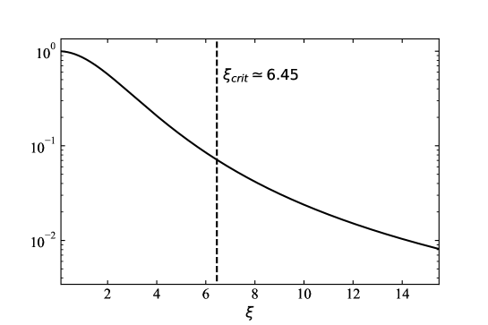
Figure 28 shows the radial density profile of the Bonnor-Ebert sphere (i.e. the numerical solution of Equation A1 and A5 ).
The total mass within the Bonnor-Ebert sphere is expressed as
| (A6) |
The Bonnor-Ebert sphere is unstable when its dimensionless radius exceeds the critical dimensionless radius of . The Bonnor-Ebert critical mass and pressure corresponding this critical values are, respectively,
| (A7) |
and
| (A9) |
Appendix B Timescales
Here, we define several important characteristic timescales to discuss the evolution of shocked clouds.
B.1 Cloud crushing time
Consider a uniform spherical cloud of radius and density in pressure equilibrium with an ambient gas of density . We focus on the case a planar shock of velocity interacts with an isothermal cloud without magnetic fields. When a shock encounters a cloud, an overpressure region and shock will be driven into the cloud. If the shock is strong, the post-shock pressure is approximately . The post-shock pressure in the cloud is of order , where is the velocity of the shock in the cloud. Assuming that these two pressures must be comparable, we
| (B1) |
where is the ratio of cloud density to ambient gas density. crushing time is the time for the shock to pass across the cloud:
| (B2) |
This is the important time scale for the evolution of the shocked cloud. In this study, we as .
B.2 Drag timescale
The shock wave accelerates cloud until it is comoving with the postshock ambient gas. Let is the mean velocity of the cloud, the velocity of the postshock ambient gas, the magnitude of the velocity of the cloud relative to velocity of the postshock ambient gas. If we consider the momentum transfer from a ambient gas with cross-section , the equation of motion of the cloud is
| (B3) |
where is the cloud mass. This equation the characteristic drag timescale as
| (B4) |
B.3 Destruction timescale
After the shock wave has swept over the cloud, the shocked cloud is subject to Kelvin-Helmholtz and Rayleigh-Taylor instabilities. For , the time-scale for growth of the Kelvin-Helmholtz instability is (Chandrasekhar, 1961) , where is the wave-number of perturbations and is the relative velocity between post-shock ambient gas and the cloud. Since the clouds accelerate rather slowly, is approximately equal to the velocity behind the shock . Thus, the time-scale for growth of the Kelvin -Helmholtz instability is comparable to the cloud crushing time
| (B5) |
The shortest wavelengths have the fastest growth, but wavelengths corresponding to are most disruptive.
The timescale an acceleration , corresponding to a growth timescale of Rayleigh-Taylor instabilities given by (Chandrasekhar, 1961). Thus, the Rayleigh-Taylor timescale is also comparable to the cloud crushing time
| (B6) |
Appendix C Values employed for each model
Table 3 specifies the for each model.
| \topruleNo. a | b | c | d | e | f | h | ||
|---|---|---|---|---|---|---|---|---|
| 1 | 2.04 | 0.31 | 0.07 | 0.125 | 1.78 | 0.56 | 1.41 | 2.67 |
| 1.99 | 3.77 | |||||||
| 2.39 | 4.53 | |||||||
| 3.15 | 5.97 | |||||||
| 2 | 2.48 | 0.38 | 0.08 | 0.25 | 2.22 | 0.89 | 1.20 | 2.27 |
| 1.41 | 2.67 | |||||||
| 1.99 | 3.77 | |||||||
| 2.39 | 4.53 | |||||||
| 3.15 | 5.97 | |||||||
| 3 | 3.22 | 0.5 | 0.11 | 0.5 | 3.24 | 1.52 | 1.20 | 2.27 |
| 1.41 | 2.67 | |||||||
| 1.99 | 3.77 | |||||||
| 3.15 | 5.97 | |||||||
| 4.00 | 7.58 | |||||||
| 4.46 | 8.45 | |||||||
| 5.00 | 9.47 | |||||||
| 5.64 | 10.68 | |||||||
| 4 | 4.05 | 0.63 | 0.14 | 0.75 | 4.94 | 2.31 | 1.20 | 2.27 |
| 4.46 | 8.45 | |||||||
| 5.00 | 9.47 | |||||||
| 5.64 | 10.68 | |||||||
| 5 | 6.45 | 1.00 | 0.22 | 1.00 | 14.10 | 4.48 | 3.15 | 5.97 |
| 5.64 | 10.68 | |||||||
| 6.00 | 11.37 | |||||||
| 7.00 | 13.26 | |||||||
| 6 | 8.52 | 1.32 | 0.29 | — | 28.08 | 6.13 | 5.64 | 10.68 |
| 6.00 | 11.37 | |||||||
| 7.00 | 13.26 | |||||||
| 7 | 14.22 | 2.20 | 0.49 | — | 100.00 | 9.78 | 6.00 | 11.37 |
| 7.00 | 13.26 | |||||||
| 8 | 6.45 | 1.00 | 0.22 | 1.00 | 14.10 | 4.48 | 1.41 | 2.67 |
| 1.99 | 3.77 | |||||||
| 3.15 | 5.97 | |||||||
| 4.46 | 8.45 | |||||||
| 5.64 | 10.68 |
-
•
No.17: values for models. No.8: for turbulent models.
a ID of the initial cloud condition.
b radius of the Bonnor-Ebert sphere.
c Ratio of the dimensionless radius the critical dimensionless radius .
d Radius of the Bonnor-Ebert sphere (pc)
e Ratio of the external pressure the critical pressure . If the initial cloud is unstable (), the value is not shown.
f Ratio of cloud central density and cloud surface density .
g of the initial cloud ().
h Mach number of the propagating shock.
i shock speed (km s-1).
Appendix D Simulation results
Table 4 specifies results of simulations numerically.
| \topruleNoa | ||||
|---|---|---|---|---|
| 1 | 2.04 | 1.41 | — | — |
| 1.99 | — | — | ||
| 2.39 | — | — | ||
| 3.15 | — | — | ||
| 2 | 2.48 | 1.20 | — | — |
| 1.41 | — | — | ||
| 1.99 | 0.32 | 0.71 | ||
| 2.39 | — | — | ||
| 3.15 | — | — | ||
| 3 | 3.22 | 1.20 | — | — |
| 1.41 | 0.74 | 1.35 | ||
| 1.99 | 0.36 | 1.24 | ||
| 3.15 | 0.15 | 0.95 | ||
| 4.00 | 0.12 | 0.66 | ||
| 4.46 | — | — | ||
| 5.00 | — | — | ||
| 5.64 | — | — | ||
| 4 | 4.05 | 1.20 | 1.14 | 1.49 |
| 4.46 | 0.13 | 1.25 | ||
| 5.00 | 0.12 | 0.94 | ||
| 5.64 | — | — | ||
| 5 | 6.45 | 3.15 | 0.31 | 4.11 |
| 5.64 | 0.18 | 0.86 | ||
| 6.00 | — | — | ||
| 7.00 | — | — | ||
| 6 | 8.52 | 5.64 | 0.22 | 1.93 |
| 6.00 | — | — | ||
| 7.00 | — | — | ||
| 7 | 14.22 | 6.00 | 0.36 | 1.23 |
| 7.00 | — | — | ||
| 8 | 6.45 | 1.41 | 1.94 | 3.21 |
| 1.99 | 0.93 | 2.87 | ||
| 3.15 | 0.49 | 2.05 | ||
| 4.46 | — | — | ||
| 5.64 | — | — |
-
•
a ID of the initial cloud condition.
b radius of the Bonnor-Ebert sphere.
c Mach number of the propagating shock.
d interval from when the shock wave reaches the cloud until the sink particles are introduced (Myr). If the sink particles is not formed, the value is not shown.
e Asymptotic mass of sink particles (). If the sink particles is not formed, the value is not shown.
Appendix E Results of different dimensionless radii models
In this appendix, we show results of cases with different dimensionless radii. Figure 29 shows evolution of density ratio at different dimensionless radius. =3.22, density evolution depends on . For triggered-collapse cases, maximum density increases monotonically or after rebounding (e.g., =4.05 and =1.20 case), inducing gravitational collapse. , when is lower or higher, the maximum density increases at the beginning but decreases to lower values after rebounding without cloud collapse. For =4.05, all of them correspond to no-collapse cases.
Figure 30 and 31 show evolution of mixing and living . =3.22, larger the Mach number, the shorter the time scale of the mixture with the ambient gas. That is, in all cases, the higher the propagating shock velocity, the faster the destruction of the cloud progress.
Figure 32 and 33 show evolution of sink particles mass and accretion rates. Figure 14 shows results of each model. From =4.05 or =6.45, we can conclude that the higher the Mach number, the slower the sink particle formation begins and the lower asymptotic sink particles mass. This trend is also the same =3.22.
Appendix F Moving of sink particles and stripped clouds
Figure 34 shows the relative and velocity sink particles and stripped clouds for and 1.20, 4.46 and 5.00 cases.
 (a) =2.04
 (b) =2.48
|
 (d) =4.05
 (e) =6.45
|
 (f) =8.54
 (g) =14.22
|
 (a) =2.04
 (b) =2.48
|
 (d) =4.05
 (e) =6.45
|
 (f) =8.54
 (g) =14.22
|
 (a) =2.04
 (b) =2.48
|
 (d) =4.05
 (e) =6.45
|
 (f) =8.54
 (g) =14.22
|
 (a) =2.48
 (c) =4.05
|
 (d) =6.45
 (e) =8.54
|
 (f) =14.22
|
 (a) =2.48
 (c) =4.05
|
 (d) =6.45
 (e) =8.54
|
 (f) =14.22
|
 (a) Relative
 (b) Relative velocity
|
References
- Alves et al. (2001) Alves, J. F., Lada, C. J., & Lada, E. A. 2001, Nature, 409, 159
- Bacmann et al. (2000) Bacmann, A., André, P., Puget, J. L., et al. 2000, A&A, 361, 555. https://arxiv.org/abs/astro-ph/0006385
- Banda-Barragán et al. (2018) Banda-Barragán, W. E., Federrath, C., Crocker, R. M., & Bicknell, G. V. 2018, MNRAS, 473, 3454, doi: 10.1093/mnras/stx2541
- Bonnor (1956) Bonnor, W. B. 1956, MNRAS, 116, 351, doi: 10.1093/mnras/116.3.351
- Boss (1995) Boss, A. P. 1995, ApJ, 439, 224, doi: 10.1086/175166
- Boss et al. (2008) Boss, A. P., Ipatov, S. I., Keiser, S. A., Myhill, E. A., & Vanhala, H. A. T. 2008, ApJ, 686, L119, doi: 10.1086/593057
- Boss & Keiser (2013) Boss, A. P., & Keiser, S. A. 2013, ApJ, 770, 51, doi: 10.1088/0004-637X/770/1/51
- Bryan et al. (2014) Bryan, G. L., Norman, M. L., O’Shea, B. W., et al. 2014, ApJ, 211, 19, doi: 10.1088/0067-0049/211/2/19
- Chandrasekhar (1961) Chandrasekhar, S. 1961, Hydrodynamic and hydromagnetic stability (Courier Corporation)
- Chandrasekhar (1967) —. 1967, An introduction to the study of stellar structure
- Ebert (1955) Ebert, R. 1955, ZAp, 37, 217
- Elmegreen & Lada (1977) Elmegreen, B. G., & Lada, C. J. 1977, ApJ, 214, 725, doi: 10.1086/155302
- Falle et al. (2017) Falle, S. A. E. G., Vaidya, B., & Hartquist, T. W. 2017, MNRAS, 465, 260, doi: 10.1093/mnras/stw2795
- Foster & Boss (1996) Foster, P. N., & Boss, A. P. 1996, ApJ, 468, 784, doi: 10.1086/177735
- Fragile et al. (2005) Fragile, P. C., Anninos, P., Gustafson, K., & Murray, S. D. 2005, ApJ, 619, 327, doi: 10.1086/426313
- Furukawa et al. (2009) Furukawa, N., Dawson, J. R., Ohama, A., et al. 2009, ApJ, 696, L115, doi: 10.1088/0004-637X/696/2/L115
- Goicoechea et al. (2020) Goicoechea, J. R., Pabst, C. H. M., Kabanovic, S., et al. 2020, A&A, 639, A1, doi: 10.1051/0004-6361/202037455
- Hester & Desch (2005) Hester, J. J., & Desch, S. J. 2005, in Astronomical Society of the Pacific Conference Series, Vol. 341, Chondrites and the Protoplanetary Disk, ed. A. N. Krot, E. R. D. Scott, & B. Reipurth, 107. https://arxiv.org/abs/astro-ph/0506190
- Hockney & Eastwood (1988) Hockney, R. W., & Eastwood, J. W. 1988, Computer simulation using particles
- Iwasaki & Tsuribe (2008) Iwasaki, K., & Tsuribe, T. 2008, PASJ, 60, 125, doi: 10.1093/pasj/60.1.125
- Kandori et al. (2005) Kandori, R., Nakajima, Y., Tamura, M., et al. 2005, AJ, 130, 2166, doi: 10.1086/444619
- Kinoshita et al. (2021) Kinoshita, S. W., Nakamura, F., Nguyen-Luong, Q., et al. 2021, PASJ, 73, S300, doi: 10.1093/pasj/psaa053
- Kirk et al. (2017) Kirk, H., Friesen, R. K., Pineda, J. E., et al. 2017, ApJ, 846, 144, doi: 10.3847/1538-4357/aa8631
- Klein et al. (1994) Klein, R. I., McKee, C. F., & Colella, P. 1994, ApJ, 420, 213, doi: 10.1086/173554
- Larson (1981) Larson, R. B. 1981, MNRAS, 194, 809, doi: 10.1093/mnras/194.4.809
- Leão et al. (2009) Leão, M. R. M., de Gouveia Dal Pino, E. M., Falceta-Gonçalves, D., Melioli, C., & Geraissate, F. G. 2009, in Revista Mexicana de Astronomia y Astrofisica Conference Series, Vol. 36, Revista Mexicana de Astronomia y Astrofisica Conference Series, CD328–CD336. https://arxiv.org/abs/0810.5374
- Li et al. (2014) Li, S., Frank, A., & Blackman, E. G. 2014, MNRAS, 444, 2884, doi: 10.1093/mnras/stu1571
- Maruta et al. (2010) Maruta, H., Nakamura, F., Nishi, R., Ikeda, N., & Kitamura, Y. 2010, ApJ, 714, 680, doi: 10.1088/0004-637X/714/1/680
- Mellema et al. (2002) Mellema, G., Kurk, J. D., & Röttgering, H. J. A. 2002, A&A, 395, L13, doi: 10.1051/0004-6361:20021408
- Nakamura et al. (2006) Nakamura, F., McKee, C. F., Klein, R. I., & Fisher, R. T. 2006, ApJ, 164, 477, doi: 10.1086/501530
- O’Dell (2001) O’Dell, C. R. 2001, AJ, 122, 2662, doi: 10.1086/323720
- Ortega et al. (2004) Ortega, V. G., de la Reza, R., Jilinski, E., & Bazzanella, B. 2004, ApJ, 609, 243, doi: 10.1086/420958
- Pittard et al. (2009) Pittard, J. M., Falle, S. A. E. G., Hartquist, T. W., & Dyson, J. E. 2009, MNRAS, 394, 1351, doi: 10.1111/j.1365-2966.2009.13759.x
- Pittard & Parkin (2016) Pittard, J. M., & Parkin, E. R. 2016, MNRAS, 457, 4470, doi: 10.1093/mnras/stw025
- Poludnenko et al. (2002) Poludnenko, A. Y., Frank, A., & Blackman, E. G. 2002, ApJ, 576, 832, doi: 10.1086/341886
- Simón-Díaz et al. (2006) Simón-Díaz, S., Herrero, A., Esteban, C., & Najarro, F. 2006, A&A, 448, 351, doi: 10.1051/0004-6361:20053066
- Stolte et al. (2008) Stolte, A., Ghez, A. M., Morris, M., et al. 2008, ApJ, 675, 1278, doi: 10.1086/527027
- Stone & Norman (1992) Stone, J. M., & Norman, M. L. 1992, ApJ, 390, L17, doi: 10.1086/186361
- Truelove et al. (1997) Truelove, J. K., Klein, R. I., McKee, C. F., et al. 1997, ApJ, 489, L179, doi: 10.1086/310975
- Turk et al. (2011) Turk, M. J., Smith, B. D., Oishi, J. S., et al. 2011, The Astrophysical Journal Supplement Series, 192, 9, doi: 10.1088/0067-0049/192/1/9
- van Leer (1977) van Leer, B. 1977, Journal of Computational Physics, 23, 276, doi: 10.1016/0021-9991(77)90095-X
- Vanhala & Boss (2002) Vanhala, H. A. T., & Boss, A. P. 2002, ApJ, 575, 1144, doi: 10.1086/341356
- Vanhala & Cameron (1998) Vanhala, H. A. T., & Cameron, A. G. W. 1998, ApJ, 508, 291, doi: 10.1086/306396
- Wu et al. (2017) Wu, B., Tan, J. C., Nakamura, F., et al. 2017, ApJ, 835, 137, doi: 10.3847/1538-4357/835/2/137
- Xu & Stone (1995) Xu, J., & Stone, J. M. 1995, ApJ, 454, 172, doi: 10.1086/176475
- Yokogawa et al. (2003) Yokogawa, S., Kitamura, Y., Momose, M., & Kawabe, R. 2003, ApJ, 595, 266, doi: 10.1086/377302