TreePiece: Faster Semantic Parsing via Tree Tokenization

Sid Wang
Meta Inc. USA
[email protected]
&Akshat Shrivastava
Meta Inc. USA
[email protected]
&Sasha Livshits
Meta Inc. USA
[email protected]

Abstract

Autoregressive (AR) encoder-decoder neural networks have proved successful in many NLP problems, including Semantic Parsing – a task that translates natural language to machine-readable parse trees. However, the sequential prediction process of AR models can be slow. To accelerate AR for semantic parsing, we introduce a new technique called TreePiece that tokenizes a parse tree into subtrees and generates one subtree per decoding step. On TOPv2 benchmark, TreePiece shows $4.6$ times faster decoding speed than standard AR, and comparable speed but significantly higher accuracy compared to Non-Autoregressive (NAR).

1 Introduction

Autoregressive (AR) modeling Sutskever et al. (2014) is a commonly adopted framework in NLP where the next prediction is conditioned on the previously generated tokens. This paper focuses on AR approach for Semantic Parsing Wong (2005), an NLP task that converts a natural language utterance to a machine-interpretable symbolic representation called logical form. The sequence of actions to derive a logical form is isomorphic to a directed tree and often referred to as a parse tree Zettlemoyer and Collins (2005).

The runtime latency of AR linearly correlates to the output length and could result in low inference speed Gu et al. (2017); Wang et al. (2018). Non-Autoregressive (NAR) modeling Gu et al. (2017); Wei et al. (2019); Ma et al. (2019), on the other hand, is able to produce outputs in parallel and reduce latency by an order of magnitude Ghazvininejad et al. (2019). However, NAR performs considerably worse than its AR counterparts without extra training recipes Wang et al. (2019); Zhou and Keung (2020); Su et al. (2021). The quality benefits of AR models therefore motivates us to improve their speed, rather than exploring NAR.

Our contributions

$\bullet$ We propose a novel approach of tokenizing parse trees into large units called TreePiece units, and then building an AR model that predicts one TreePiece unit at a time, thus reducing the number of steps needed to generate a full parse tree. To the best of our knowledge, we are the first to extend subword-tokenizer algorithm to semantic trees such that each token is a subtree.

$\bullet$ We validate our approach on TOPv2 benchmark and show that TreePiece decoding is 4.6 times faster than standard AR with less than $0.2\%$ accuracy degradation, and nearly as fast as NAR with up to $0.8\%$ accuracy gains.

$\bullet$ We provide theoretical proofs to support our main algorithms and their variants.

2 Methods

2.1 Parse tree

In this paper, we utilize the hierarchical semantic representations based on intent and slot Gupta et al. (2018), allowing for modeling complex compositional queries in task-oriented dialog systems. See Figure 1 (LHS) for an example. We begin with a few recurring definitions.

Definition 2.1 (Ontology).

A parse tree node is called an ontology iff it represents an intent/slot, prefixed by in: and sl: respectively.

Definition 2.2 (Skeleton).

The skeleton of a parse tree is the subtree that consists of all ontologies.

Definition 2.3 (Utterance leaf).

A text-span node is called an utterance leaf iff its parent is a slot¹¹1We adopt the decoupled form proposed in Aghajanyan et al. (2020), which simplifies compositional representations by ignoring text spans that are not utterance leaves..

2.2 TreePiece tokenizer algorithm

We propose the algorithm to train a TreePiece tokenizer that partitions a skeleton into subtrees.

Definition 2.4 (TreePiece vocabulary).

The minimal open vocabulary of all possible subtree units returned from a TreePiece tokenizer is called a TreePiece vocabulary. We refer to each element in a TreePiece vocabulary as a TreePiece unit.

Definition 2.5 (TreePiece simplex).

Let $\mathcal{V}$ be a TreePiece vocabulary and $t$ be any TreePiece unit. A TreePiece simplex $\boldsymbol{p}$ is a mapping from $\mathcal{V}$ to the unit interval $[0,1]$ such that $\sum_{t\in\mathcal{V}}\boldsymbol{p}(t)=1$ .

Our training proceeds in two stages: (1) generating TreePiece vocabulary from a training corpus; (2) optimizing the TreePiece simplex via an Expectation-Maximization (EM) algorithm.

2.2.1 Vocabulary generation

This stage resembles the merging operation in Byte Pair Encoding (BPE) Gage (1994); Sennrich et al. (2015). Given a training corpus, denote its skeletons by $\mathscr{S}$ . We initialize the TreePiece vocabulary $\mathcal{V}$ as the set of ontologies extracted from $\mathscr{S}$ and $\mathcal{F}_{0}$ as the map between ontologies and their frequencies in $\mathscr{S}$ . Now repeat the steps below until $\mathcal{V}$ reaches a pre-determined size:

•

Count the frequencies of all adjacent but unmerged TreePiece unit pairs in $\mathscr{S}$ . Find the most frequent pair $p^{*}$ and its frequency $n^{*}$ .
•

Merge $p^{*}$ in every $S\in\mathscr{S}$ that contains $p^{*}$ , add $p^{*}$ to $\mathcal{V}$ , and update $\mathcal{F}_{0}$ with $\mathcal{F}_{0}(p^{*})=n^{*}$ .

Refer to caption — Figure 1: Illustration of tokenizing parse tree/assembling TreePiece units with the placeholder design for given utterance “*Remind me to send Susan an email about the meeting tonight*”.

2.2.2 EM algorithm

Briefly speaking, we initialize the TreePiece simplex $\boldsymbol{p}_{0}$ by setting $\boldsymbol{p}_{0}(t)$ (for each $t\in\mathcal{V}$ ) to be the normalized frequency ${\mathcal{F}_{0}(t)}/{\sum_{\tau\in\mathcal{V}}\mathcal{F}_{0}(\tau)}$ , and will iteratively derive $\boldsymbol{{p}_{i+1}}$ for $i=0,1,2,\cdots$ according to the following inductive formula:

\boldsymbol{{p}_{i+1}}=\text{argmax}_{\boldsymbol{{p}}}\sum_{S\in\mathscr{S}}\mathbb{E}\big{[}\log\mathbb{P}(S,\pi;\boldsymbol{{p}})\big{\rvert}S;\boldsymbol{{p}_{i}}\big{]}.

(1)

Here $\pi$ denotes a partition of skeleton $S$ . In general, problem (1) is NP-hard as it involves summing over $\Pi_{S}$ , the set of all possible partitions of $S$ :

\displaystyle\begin{split}&\mathbb{E}\big{[}\log\mathbb{P}(S,\pi;\boldsymbol{{p}})\big{\rvert}S;\boldsymbol{{p}_{i}}\big{]}\\ =&\sum_{\pi\in\Pi_{S}}\log\mathbb{P}(S,\pi;\boldsymbol{{p}})\cdot\frac{\mathbb{P}(S,\pi;\boldsymbol{{p}_{i}})}{\mathbb{P}(S;\boldsymbol{{p}_{i}})}\end{split}

(2)

To solve (1) in polynomial time, we impose the following assumption on the joint distribution:

\mathbb{P}(S,\pi;\boldsymbol{p})\propto\left\{\begin{array}[]{ c l }\prod_{\tau\in\pi}\boldsymbol{p}(\tau)&\text{if }\pi=\pi_{S}(\boldsymbol{p})\\ 0&\textrm{otherwise,}\end{array}\right.

(3)

where $\pi_{S}(\boldsymbol{p})=\text{argmax}_{\pi\in\Pi_{S}}{\prod}_{\tau\in\pi}\boldsymbol{p}(\tau).$ Applying (3), we see that all but one summand in (LABEL:cond) vanish. Algorithm 1 outlines the EM process to solve (1).

Algorithm 1 EM algorithm

Choose

N_{0}\in\mathbb{N}^{+},\epsilon_{0}>0

; initialize

i\leftarrow 0

\Delta\leftarrow+\infty

\mathcal{L}_{\text{prev}}\leftarrow-\infty

while

i<N_{0}

and

\Delta>\epsilon_{0}

\mathcal{L}_{\text{curr}}\leftarrow 0

\mathcal{F}^{*}\leftarrow\text{Zero function on $\mathcal{V}$}

for

S\in\mathscr{S}

Compute

\pi_{S}(\boldsymbol{p}_{i})

and

\mathbb{P}(S;\boldsymbol{p}_{i})

\triangleright

E-step

\mathcal{L}_{\text{curr}}\leftarrow\mathcal{L}_{\text{curr}}+\log\mathbb{P}(S;\boldsymbol{p}_{i})

for

t\in\pi_{S}(\boldsymbol{p}_{i})

\mathcal{F}^{*}(t)\leftarrow\mathcal{F}^{*}(t)+1

for

t\in\mathcal{V}

\boldsymbol{p}_{i+1}(t)\leftarrow\frac{\mathcal{F}^{*}(t)}{\sum_{\tau\in\mathcal{V}}\mathcal{F}^{*}(\tau)}

\triangleright

M-step

i\leftarrow i+1,\Delta\leftarrow\mathcal{L}_{\text{curr}}-\mathcal{L}_{\text{prev}}

\mathcal{L}_{\text{prev}}\leftarrow\mathcal{L}_{\text{curr}}

In the E-step of Algorithm 1 we use a Viterbi-type algorithm Viterbi (1967), given in Appendix A.

The following Theorem claims that Algorithm 1 solves (1). We defer its proof to Appendix B.

Theorem 2.6.

Let $\boldsymbol{p}_{0},\boldsymbol{p}_{1},\boldsymbol{p}_{2},\cdots$ be the sequence of TreePiece simplices obtained from Algorithm 1. If (3) holds, then $\boldsymbol{p}_{i+1}$ solves the optimization problem (1), for $i\geq 0$ . Especially, $\sum_{S\in\mathscr{S}}\log\mathbb{P}(S;\boldsymbol{p}_{i})$ is monotonically non-decreasing in $i$ .

2.3 Modeling

We describe the model that generates parse tree components and the method to piece them together.

2.3.1 Modeling mechanism

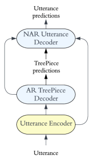
As illustrated in Figure 2, an encoder computes the hidden states of a given utterance, then an AR decoder consumes the encoder hidden states and generate TreePiece units autoregressively. The technique in Subsection 2.3.2 will allow us to put these units together and obtain a full skeleton. The skeleton then uniquely determines the numbers and positions of all utterance leaves (see Figure 1), which offers us the convenience to use an NAR decoder to generate all utterance leaves within one step.

2.3.2 Assemble TreePiece units

Unlike subword-tokenization, where original sentence can be trivially recovered from subword units via string concatenation, there is no canonical way to reassemble TreePiece units. To overcome this issue, we allow TreePiece units to have placeholders²²2Finding all possible placeholder patterns is NP-hard and unnecessary. In Appendix D we provide a practical solution., and require that two units can only be joined at a placeholder node. This design provides a unique way to glue a sequence of ordered (e.g. pre/level-ordered) TreePiece units, as shown in Figure 1.

3 Experiments

3.1 Datasets

We train, validate, and test our approach on the publicly available benchmark TOPv2 Chen et al. (2020), a multi-domain task-oriented semantic parsing dataset. The dataset provides a training/validation/test split. Throughout our experiments, we use the training split to train the models, the validation split for earlystopping, model checkpointing, and hyperparameter tuning, and the test split to report the best model’s performance.

3.2 Metrics

We evaluate the model performance on two metrics: Exact Match (EM) respectively Exact Match of Skeleton (EM-S), defined to be the percentage of utterances whose logical forms respectively skeletons are correctly predicted Shrivastava et al. (2022).

3.3 Baselines

We compare our approach against 2 baselines: AR and NAR. Both baselines are sequence-to-sequence (seq2seq) that produces subword units of serialized logical forms. Their output space consists of ontologies (prefixed by left bracket “[”), utterance leaves³³3We represent utterance leaves in span-pointers Shrivastava et al. (2021) form to simplify the parsing task., and right bracket “]”.
AR baseline admits a standard AR structure. It has an autoregressive decoder that generates serialized logical forms by producing one token at a time.
NAR baseline adopts mask-predict Ghazvininejad et al. (2019) with beam size $1$ , which predicts the output length first and then generates all tokens in one step using a non-autoregressive decoder.

4 Results

TreePiece

NAR

EM (%)

86.78

86.99

86.22

EM-S(%)

89.14

89.13

88.44

Decoding (ms)

152

Inference (ms)

196

Table 1: Quality and latency of all models on TOPv2

We train each model with $3$ random seeds, and report the averaged EM/EM-S test scores. To obtain latency, we infer the trained models on the test split of TOPv2 dataset with CPU and report the averaged milliseconds over all samples. We defer the model configurations, training details, and comparisons with prior work to Appendix E.

4.1 Quality

As shown in Table 1, TreePiece model sees $0.7\%$ relative improvements over NAR and $0.2\%$ relative degradation from AR in terms of EM, while achieving the best EM-S score among all approaches, especially showing $0.8\%$ relative improvement over NAR. We attribute TreePiece’s high quality on skeleton predictions to its ability to respect the tree structure of logical forms and generating $100\%$ valid outputs by design so that the model can better focus on utterance-understanding without being distracted by any structure issue.

4.2 Latency

TreePiece makes decoding $4.6$ times faster and overall inference $2.7$ times faster than AR, with less than $10\%$ latency growth compared to NAR (see Table 1). The acceleration effects are illustrated in 3, showing that TreePiece substantially reduces the number of decoding steps and thereby requires fewer passes through decoder layers.

Related work Autoregressive modeling have been used in a range of Semantic Parsing works Tai et al. (2015); Cheng et al. (2017b); Dong and Lapata (2018). Especially, the Sequence-to-Tree scheme was adopted by Dong and Lapata (2016). To speed up the inference time, Non-autoregressive modeling were introduced to the field of Machine Translation Gu et al. (2017); Lee et al. (2018); Libovický and Helcl (2018), and later become popular in Semantic Parsing as well Ghazvininejad et al. (2019); Babu et al. (2021); Shrivastava et al. (2021). However, to match the quality of AR, extra training stages are necessary such as Knowledge Distillation from AR models Gu et al. (2017); Lee et al. (2018); Wei et al. (2019); Stern et al. (2019). On the other hand, Rubin and Berant (2020) improves AR decoding’s efficiency via Bottom-Up Parsing Cheng et al. (2017a). This paper takes a completely different path from all previous work by extending the subword tokenization algorithms Nagata (1994a); Scott (2002); Sennrich et al. (2015); Kudo (2018); Kudo and Richardson (2018) to trees.

Conclusion

This paper proposes a novel technique to speed up Autoregressive modeling for Semantic Parsing via tokenizing parse trees into subtrees. We provide thorough elucidations and theoretical supports for our technique, and demonstrate significant improvements in terms of speed and quality over common baselines on the TOPv2 benchmark.

References

Aghajanyan et al. (2020) Armen Aghajanyan, Jean Maillard, Akshat Shrivastava, Keith A. Diedrick, Mike Haeger, Haoran Li, Yashar Mehdad, Ves Stoyanov, Anuj Kumar, Mike Lewis, and S. Gupta. 2020. Conversational semantic parsing. In Conference on Empirical Methods in Natural Language Processing.
Babu et al. (2021) Arun Babu, Akshat Shrivastava, Armen Aghajanyan, Ahmed Aly, Angela Fan, and Marjan Ghazvininejad. 2021. Non-autoregressive semantic parsing for compositional task-oriented dialog. In North American Chapter of the Association for Computational Linguistics.
Chen et al. (2020) Xilun Chen, Asish Ghoshal, Yashar Mehdad, Luke Zettlemoyer, and S. Gupta. 2020. Low-resource domain adaptation for compositional task-oriented semantic parsing. In Conference on Empirical Methods in Natural Language Processing.
Cheng et al. (2017a) Jianpeng Cheng, Siva Reddy, Vijay A. Saraswat, and Mirella Lapata. 2017a. Learning an executable neural semantic parser. Computational Linguistics, 45:59–94.
Cheng et al. (2017b) Jianpeng Cheng, Siva Reddy, Vijay A. Saraswat, and Mirella Lapata. 2017b. Learning structured natural language representations for semantic parsing. ArXiv, abs/1704.08387.
Devlin et al. (2019) Jacob Devlin, Ming-Wei Chang, Kenton Lee, and Kristina Toutanova. 2019. Bert: Pre-training of deep bidirectional transformers for language understanding. ArXiv, abs/1810.04805.
Dong and Lapata (2016) Li Dong and Mirella Lapata. 2016. Language to logical form with neural attention. ArXiv, abs/1601.01280.
Dong and Lapata (2018) Li Dong and Mirella Lapata. 2018. Coarse-to-fine decoding for neural semantic parsing. In Annual Meeting of the Association for Computational Linguistics.
Gage (1994) Philip Gage. 1994. A new algorithm for data compression. The C Users Journal archive, 12:23–38.
Ghazvininejad et al. (2019) Marjan Ghazvininejad, Omer Levy, Yinhan Liu, and Luke Zettlemoyer. 2019. Constant-time machine translation with conditional masked language models. ArXiv, abs/1904.09324.
Gu et al. (2017) Jiatao Gu, James Bradbury, Caiming Xiong, Victor O. K. Li, and Richard Socher. 2017. Non-autoregressive neural machine translation. ArXiv, abs/1711.02281.
Gupta et al. (2018) S. Gupta, Rushin Shah, Mrinal Mohit, Anuj Kumar, and Mike Lewis. 2018. Semantic parsing for task oriented dialog using hierarchical representations. In Conference on Empirical Methods in Natural Language Processing.
Kingma and Ba (2014) Diederik P. Kingma and Jimmy Ba. 2014. Adam: A method for stochastic optimization. CoRR, abs/1412.6980.
Kudo (2018) Taku Kudo. 2018. Subword regularization: Improving neural network translation models with multiple subword candidates. In Annual Meeting of the Association for Computational Linguistics.
Kudo and Richardson (2018) Taku Kudo and John Richardson. 2018. Sentencepiece: A simple and language independent subword tokenizer and detokenizer for neural text processing. In Conference on Empirical Methods in Natural Language Processing.
Lee et al. (2018) Jason Lee, Elman Mansimov, and Kyunghyun Cho. 2018. Deterministic non-autoregressive neural sequence modeling by iterative refinement. In Conference on Empirical Methods in Natural Language Processing.
Libovický and Helcl (2018) Jindřich Libovický and Jindřich Helcl. 2018. End-to-end non-autoregressive neural machine translation with connectionist temporal classification. In Proceedings of the 2018 Conference on Empirical Methods in Natural Language Processing, pages 3016–3021, Brussels, Belgium. Association for Computational Linguistics.
Liu et al. (2019) Yinhan Liu, Myle Ott, Naman Goyal, Jingfei Du, Mandar Joshi, Danqi Chen, Omer Levy, Mike Lewis, Luke Zettlemoyer, and Veselin Stoyanov. 2019. Roberta: A robustly optimized bert pretraining approach. ArXiv, abs/1907.11692.
Ma et al. (2019) Xuezhe Ma, Chunting Zhou, Xian Li, Graham Neubig, and Eduard H. Hovy. 2019. Flowseq: Non-autoregressive conditional sequence generation with generative flow. ArXiv, abs/1909.02480.
Nagata (1994a) Masaaki Nagata. 1994a. A stochastic Japanese morphological analyzer using a forward-DP backward-A* n-best search algorithm. In COLING 1994 Volume 1: The 15th International Conference on Computational Linguistics, Kyoto, Japan.
Nagata (1994b) Masaaki Nagata. 1994b. A stochastic japanese morphological analyzer using a forward-dp backward-a* n-best search algorithm. In International Conference on Computational Linguistics.
Rongali et al. (2020) Subendhu Rongali, Luca Soldaini, Emilio Monti, and Wael Hamza. 2020. Don’t parse, generate! a sequence to sequence architecture for task-oriented semantic parsing. Proceedings of The Web Conference 2020.
Rubin and Berant (2020) Ohad Rubin and Jonathan Berant. 2020. Smbop: Semi-autoregressive bottom-up semantic parsing. In North American Chapter of the Association for Computational Linguistics.
Scott (2002) Steven L Scott. 2002. Bayesian methods for hidden markov models. Journal of the American Statistical Association, 97(457):337–351.
Senior et al. (2013) Andrew W. Senior, Georg Heigold, Marc’Aurelio Ranzato, and Ke Yang. 2013. An empirical study of learning rates in deep neural networks for speech recognition. 2013 IEEE International Conference on Acoustics, Speech and Signal Processing, pages 6724–6728.
Sennrich et al. (2015) Rico Sennrich, Barry Haddow, and Alexandra Birch. 2015. Neural machine translation of rare words with subword units. ArXiv, abs/1508.07909.
Shrivastava et al. (2021) Akshat Shrivastava, Pierce I-Jen Chuang, Arun Babu, Shrey Desai, Abhinav Arora, Alexander Zotov, and Ahmed Aly. 2021. Span pointer networks for non-autoregressive task-oriented semantic parsing. In Conference on Empirical Methods in Natural Language Processing.
Shrivastava et al. (2022) Akshat Shrivastava, Shrey Desai, Anchit Gupta, Ali Mamdouh Elkahky, Aleksandr Livshits, Alexander Zotov, and Ahmed Aly. 2022. Retrieve-and-fill for scenario-based task-oriented semantic parsing. ArXiv, abs/2202.00901.
Stern et al. (2019) Mitchell Stern, William Chan, Jamie Ryan Kiros, and Jakob Uszkoreit. 2019. Insertion transformer: Flexible sequence generation via insertion operations. In International Conference on Machine Learning.
Su et al. (2021) Yixuan Su, Deng Cai, Yan Wang, David Vandyke, Simon Baker, Piji Li, and Nigel Collier. 2021. Non-autoregressive text generation with pre-trained language models. In Conference of the European Chapter of the Association for Computational Linguistics.
Sutskever et al. (2014) Ilya Sutskever, Oriol Vinyals, and Quoc V. Le. 2014. Sequence to sequence learning with neural networks. In NIPS.
Tai et al. (2015) Kai Sheng Tai, Richard Socher, and Christopher D. Manning. 2015. Improved semantic representations from tree-structured long short-term memory networks. ArXiv, abs/1503.00075.
Vaswani et al. (2017) Ashish Vaswani, Noam M. Shazeer, Niki Parmar, Jakob Uszkoreit, Llion Jones, Aidan N. Gomez, Lukasz Kaiser, and Illia Polosukhin. 2017. Attention is all you need. ArXiv, abs/1706.03762.
Viterbi (1967) Andrew J. Viterbi. 1967. Error bounds for convolutional codes and an asymptotically optimum decoding algorithm. IEEE Trans. Inf. Theory, 13:260–269.
Wang et al. (2018) Chunqi Wang, Ji Zhang, and Haiqing Chen. 2018. Semi-autoregressive neural machine translation. In Conference on Empirical Methods in Natural Language Processing.
Wang et al. (2019) Yiren Wang, Fei Tian, Di He, Tao Qin, ChengXiang Zhai, and Tie-Yan Liu. 2019. Non-autoregressive machine translation with auxiliary regularization. In AAAI Conference on Artificial Intelligence.
Wei et al. (2019) Bingzhen Wei, Mingxuan Wang, Hao Zhou, Junyang Lin, and Xu Sun. 2019. Imitation learning for non-autoregressive neural machine translation. ArXiv, abs/1906.02041.
Wong (2005) Yuk Wah Wong. 2005. Learning for semantic parsing using statistical machine translation techniques.
Zettlemoyer and Collins (2005) Luke Zettlemoyer and Michael Collins. 2005. Learning to map sentences to logical form: Structured classification with probabilistic categorial grammars. ArXiv, abs/1207.1420.
Zhou and Keung (2020) Jiawei Zhou and Phillip Keung. 2020. Improving non-autoregressive neural machine translation with monolingual data. In Annual Meeting of the Association for Computational Linguistics.

Appendix A Appendix

Algorithm 2 outlines the Viterbi-type forward-backward Nagata (1994b) algorithm used in the EM procedure (ref. Algorithm 1) to compute the optimal tokenization and its probability for given skeleton $S$ . We first obtain the set of all subtrees of $S$ that share the same root as $S$ denoted by $\mathcal{T}$ . For convenience, we assume that $\mathcal{T}$ is graded by depth, such that $\mathcal{T}_{d}\subseteq\mathcal{T}$ denotes the set of all depth- $d$ -subtrees. Next, we call GetInitLogProbs to initialize the log probability function on $\mathcal{T}$ as follows:

\mathscr{L}(\mathfrak{t})=\begin{cases}\log\boldsymbol{p}(\mathfrak{t})&\text{ if }\mathfrak{t}\in\mathcal{V},\\ -\infty&\text{ otherwise}.\end{cases}

where $\mathcal{V}$ is the TreePiece vocabulary and $\boldsymbol{p}$ the TreePiece simplex.

Algorithm 2 Forward-backward algorithm

TreePiece vocabulary

\mathcal{V}

, TreePiece simplex

\boldsymbol{p}

, and skeleton

S

Parition

\pi_{S}(\boldsymbol{p})

and probability

\mathbb{P}(S;\boldsymbol{p})

\mathcal{T}\leftarrow

All subtrees of

S

with the same root.

\mathscr{L}\leftarrow

GetInitLogProbs

(\boldsymbol{p})

\mathscr{P}\leftarrow

Constant map from

\mathcal{T}

to BOS token

d_{\text{max}}\leftarrow\text{Depth of {S}}

// Forward begins

for

d=1,2,\cdots,d_{\text{max}}

for

\mathfrak{t}\in\mathcal{T}_{d}

for

d^{\prime}=1,2,\cdots,d

for

\mathfrak{t}^{\prime}\in\texttt{Filter}(\mathcal{T}_{d^{\prime}},\mathfrak{t})

\Delta^{*}\leftarrow

\mathfrak{t}^{\prime}\Delta\mathfrak{t}

L^{*}\leftarrow\mathscr{L}(\mathfrak{t}^{\prime})+\sum_{\tau\in\Delta^{*}}\log\boldsymbol{p}(\tau)

L^{*}>\mathscr{L}(\mathfrak{t})

then

\mathscr{L}(\mathfrak{t})\leftarrow L^{*}

\mathscr{P}(\mathfrak{t})\leftarrow\mathfrak{t}^{\prime}

\mathbb{P}(S;\boldsymbol{p})\leftarrow\exp(\mathscr{L}(S))

// Forward ends

\mathfrak{t}_{\text{curr}}\leftarrow S

\pi_{S}(\boldsymbol{p})\leftarrow\emptyset

// Backward begins

while

\mathfrak{t}_{\text{curr}}\neq\texttt{BOS}

token, do

\mathfrak{t}_{\text{prev}}\leftarrow\mathscr{P}(\mathfrak{t}_{\text{curr}})

\Delta^{*}\leftarrow\mathfrak{t}_{\text{prev}}\Delta\mathfrak{t}_{\text{curr}}

\pi_{S}(\boldsymbol{p})\leftarrow\pi_{S}(\boldsymbol{p})\bigcup\Delta^{*}

\mathfrak{t}_{\text{curr}}\leftarrow\mathfrak{t}_{\text{prev}}

\pi_{S}(\boldsymbol{p})\leftarrow\pi_{S}(\boldsymbol{p})\bigcup\{\mathfrak{t}_{\text{curr}}\}

// Backward ends

return

\pi_{S}(\boldsymbol{p}),\mathbb{P}(S;\boldsymbol{p})

The forward step uses dynamic programming inductive on tree-depth to update all subtrees’ log-probabilities and eventually obtain $\mathbb{P}(S;\boldsymbol{p})$ – the probability of the skeleton $S$ . The forward step also returns a map $\mathscr{P}$ that stores for each $\mathfrak{t}\in\mathcal{T}$ the optimal position of its previous partition. Then in the backward step we can backtrack along the path $S$ , $\mathscr{P}(S),\mathscr{P}(\mathscr{P}(S)),\cdots$ to recover the optimal partition $\pi_{S}(\boldsymbol{p})$ . Note that for dynamic programming’s efficiency we apply a Filter $(\cdot,\mathfrak{t})$ method to narrow down the subtrees to those $\mathfrak{t}^{\prime}$ such that (1) $\mathfrak{t}^{\prime}$ is a subtree of $\mathfrak{t}$ , (2) the set difference $\mathfrak{t}^{\prime}\Delta\mathfrak{t}$ has exactly one connected component and it is a TreePiece unit.

Appendix B Appendix

For convenience we adopt the following notations.

Notation B.1.

Let $\boldsymbol{p}$ be a TreePiece simplex and $\pi\eqqcolon[\tau_{1},\cdots,\tau_{k}]$ be a partition where each $\tau_{i}$ is a TreePiece unit. Define $\boldsymbol{p}(\pi)\eqqcolon\prod_{\tau\in\pi}\boldsymbol{p}(\tau)$ .

Notation B.2.

Let $\pi\eqqcolon[\tau_{1},\cdots,\tau_{k}]$ be a partition and $\tau$ be any TreePiece unit. Define $n(\pi,\tau)\eqqcolon\sum_{\tau_{i}\in\pi}\mathbbm{1}_{\tau=\tau_{i}}$ . In other words, $n(\pi,\tau)$ is the number of appearances of $\tau$ in $\pi$ .

Now we introduce a general hypothesis and will prove a key lemma under this hypothesis.

Hypothesis B.1.

The joint distribution of skeleton $S$ and partition $\pi$ satisfies the following rule,

\mathbb{P}(S,\pi;\boldsymbol{p})\propto\left\{\begin{array}[]{ l l }\prod_{\tau\in\pi}\boldsymbol{p}(\tau)\cdot\chi(\pi,\boldsymbol{p})\text{ if }\pi\in\Pi_{S}\\ 0\textrm{ otherwise,}\end{array}\right.

(4)

where $\chi:\Pi_{S}\times[0,1]^{|\mathcal{V}|}\to\{0,1\}$ is locally smooth almost everywhere (under Lebesgue measure on $[0,1]$ ). In other words, for $a.e.$ $\boldsymbol{p}\in[0,1]^{|\mathcal{V}|}$ and every $\pi\in\Pi_{S}$ there exists a neighborhood $B_{\epsilon}(\boldsymbol{p})$ where $\chi(\pi,\cdot)$ is constant.

Remark B.1.

Assumption (3) is a special case of hypothesis B.1, where $\chi(\pi,\boldsymbol{p})=1$ if $\pi=\pi_{S}(\boldsymbol{p})$ and $0$ otherwise.

Remark B.2.

Without loss of generality, in equations (3) and (4) we replace the symbol “ $\propto$ ” with “ $=$ ”, which otherwise complicates all formulae expressions with a non-essential scalar constant.

Lemma B.1.

Under Hypothesis B.1, $\boldsymbol{p}_{k+1}$ is a solution to (1) iff the following holds $\forall\tau^{*}\in\mathcal{V}$ :

\boldsymbol{p}_{k+1}(\tau^{*})=\frac{\sum_{S\in\mathscr{S}}\mathbb{E}_{\Pi_{S}}[n(\pi,\tau^{*})|S;\boldsymbol{p}_{k}]}{\sum_{\tau\in\mathcal{V}}\sum_{S\in\mathscr{S}}\mathbb{E}_{\Pi_{S}}[n(\pi,\tau)|S;\boldsymbol{p}_{k}]}.

(5)

proof of Theorem 2.6 assuming Lemma B.1 holds.

By following the E-step of Algorithm 1, we can express the frequency $\mathcal{F}^{*}(t)$ as

\sum_{S\in\mathscr{S}}\sum_{\tau\in\pi_{S}(\boldsymbol{p}_{i})}\mathbbm{1}_{\tau=t}=\sum_{S\in\mathscr{S}}n(\pi_{S}(\boldsymbol{p}_{i}),t).

(6)

Assumption 3 says that the probability measure $\mathbb{P}(\pi|S;\boldsymbol{p}_{k})$ is supported on the singleton $\pi_{S}(\boldsymbol{p}_{i})$ , therefore the following holds for all $\tau\in\mathcal{V}$ :

n(\pi_{S}(\boldsymbol{p}_{i}),\tau)=\mathbb{E}_{\Pi_{S}}[n(\pi,\tau)|S;\boldsymbol{p}_{k}].

(7)

Now inserting the identity (7) to the right hand side of equation (6) we obtain

\mathcal{F}^{*}(t)=\sum_{S\in\mathscr{S}}\mathbb{E}_{\Pi_{S}}[n(\pi,t)|S;\boldsymbol{p}_{k}].

(8)

Next, Inserting (8) to the M-step in Algorithm 1, we have

\boldsymbol{p}_{k+1}(t)=\frac{\sum_{S\in\mathscr{S}}\mathbb{E}_{\Pi_{S}}[n(\pi,t)|S;\boldsymbol{p}_{k}]}{\sum_{\tau\in\mathcal{V}}\sum_{S\in\mathscr{S}}\mathbb{E}_{\Pi_{S}}[n(\pi,\tau)|S;\boldsymbol{p}_{k}]}.

(9)

Invoking Lemma B.1, we see that $\boldsymbol{p}_{k+1}$ is the solution to problem (1), which proves the first conclusion in Theorem 2.6.

Secondly, the monotonicity of $\log\mathbb{P}(S;\boldsymbol{p}_{i})$ can be achieved as follows:

\displaystyle\begin{split}&\sum_{S\in\mathscr{S}}\log\mathbb{P}(S;\boldsymbol{p}_{k+1})\\ =&\sum_{S\in\mathscr{S}}\log\mathbb{P}(S,\pi_{S}(\boldsymbol{p}_{k+1});\boldsymbol{p}_{k+1})\\ =&\sum_{S\in\mathscr{S}}\boldsymbol{p}_{k+1}(\pi_{S}(\boldsymbol{p}_{k+1}))\\ \geq&\sum_{S\in\mathscr{S}}\boldsymbol{p}_{k+1}(\pi_{S}(\boldsymbol{p}_{k}))\\ =&\sum_{S\in\mathscr{S}}\log\mathbb{P}(S,\pi_{S}(\boldsymbol{p}_{k});\boldsymbol{p}_{k+1})\\ =&\sum_{S\in\mathscr{S}}\mathbb{E}[\log\mathbb{P}(S,\pi_{S}(\boldsymbol{p}_{k});\boldsymbol{p}_{k+1})|S;\boldsymbol{p}_{k}]\\ \geq&\sum_{S\in\mathscr{S}}\mathbb{E}[\log\mathbb{P}(S,\pi_{S}(\boldsymbol{p}_{k});\boldsymbol{p}_{k})|S;\boldsymbol{p}_{k}]\\ =&\sum_{S\in\mathscr{S}}\boldsymbol{p}_{k}(\pi_{S}(\boldsymbol{p}_{k}))\\ =&\sum_{S\in\mathscr{S}}\log\mathbb{P}(S,\pi_{S}(\boldsymbol{p}_{k});\boldsymbol{p}_{k})\\ =&\sum_{S\in\mathscr{S}}\log\mathbb{P}(S;\boldsymbol{p}_{k}).\end{split}

(10)

Here, all equalities are consequences of Assumption 3, the first inequality follows from the definition of $\pi_{S}(\boldsymbol{p}_{k+1})$ , and the second inequality uses the maximization property of $\boldsymbol{p}_{k+1}$ :

\boldsymbol{p}_{k+1}=\text{argmax}_{\boldsymbol{p}}\sum_{S\in\mathscr{S}}\mathbb{E}[\log\mathbb{P}(S,\pi_{S}(\boldsymbol{p}_{k});\boldsymbol{p})|S;\boldsymbol{p}_{k}].

(11)

Thus concludes Theorem 2.6. ∎

To complete the proof of Theorem 2.6 it suffices to prove Lemma B.1.

proof of Lemma B.1.

Consider the following Lagrange multiplier of problem (1):

\displaystyle\begin{split}\mathcal{L}(\boldsymbol{p},\lambda)=&\sum_{S\in\mathscr{S}}\mathbb{E}\big{[}\log\mathbb{P}(S,\pi;\boldsymbol{{p}})\big{\rvert}S;\boldsymbol{{p}_{k}}\big{]}\\ &+\lambda(\sum_{\tau\in\mathcal{V}}\boldsymbol{p}(\tau)-1).\end{split}

(12)

Plugging (4) into the above equation, we get

\displaystyle\begin{split}&\sum_{S\in\mathscr{S}}\sum_{\pi\in\Pi_{S}}\log\boldsymbol{p}(\pi)\cdot\mathbb{P}(\pi\big{\rvert}S;\boldsymbol{p}_{k})\\ +&\sum_{S\in\mathscr{S}}\sum_{\pi\in\Pi_{S}}\log\chi(\pi,\boldsymbol{p})\cdot\mathbb{P}(\pi\big{\rvert}S;\boldsymbol{p}_{k})\\ +&\lambda(\sum_{\tau\in\mathcal{V}}\boldsymbol{p}(\tau)-1)\\ \coloneqq&\text{I}+\text{II}+\text{III}.\end{split}

(13)

Inserting equation (LABEL:terms) to the following identity:

\nabla_{\boldsymbol{p},\lambda}\mathcal{L}=\boldsymbol{0},

(14)

we obtain for each $\tau^{*}\in\mathcal{V}$ that

\displaystyle\begin{split}\sum_{S\in\mathscr{S}}\sum_{\pi\in\Pi_{S}}\frac{n(\pi,\tau^{*})}{\boldsymbol{p}(\tau^{*})}\cdot\mathbb{P}(\pi\big{\rvert}S;\boldsymbol{p}_{k})+\lambda=0.\end{split}

(15)

Note the locally constant assumption in Hypothesis B.1 makes the derivative of term II vanishes $a.e.$ . Identity (15) then allows us to solve for $\boldsymbol{p}(\tau^{*})$ :

\boldsymbol{p}(\tau^{*})=-\frac{1}{\lambda}\cdot\sum_{S\in\mathscr{S}}\sum_{\pi\in\Pi_{S}}n(\pi,\tau^{*})\cdot\mathbb{P}(\pi\big{\rvert}S;\boldsymbol{p}_{k}).

(16)

Next, using the simplex property $\sum_{\tau\in\mathcal{V}}\boldsymbol{p}(\tau)=1$ and summing up (16) over $\mathcal{V}$ , we find $\lambda$ :

-\frac{1}{\sum_{\tau\in\mathcal{V}}\sum_{S\in\mathscr{S}}\sum_{\pi\in\Pi_{S}}n(\pi,\tau)\cdot\mathbb{P}(\pi\big{\rvert}S;\boldsymbol{p}_{k})}.

(17)

Plugging the above value of $\lambda$ back to (16), we obtain the final expression of $\boldsymbol{p}(\tau^{*})$ :

\displaystyle\begin{split}&\frac{\sum_{S\in\mathscr{S}}\sum_{\pi\in\Pi_{S}}n(\pi,\tau^{*})\cdot\mathbb{P}(\pi\big{\rvert}S;\boldsymbol{p}_{k})}{\sum_{\tau\in\mathcal{V}}\sum_{S\in\mathscr{S}}\sum_{\pi\in\Pi_{S}}n(\pi,\tau)\cdot\mathbb{P}(\pi\big{\rvert}S;\boldsymbol{p}_{k})}\\ =&\frac{\sum_{S\in\mathscr{S}}\mathbb{E}\big{[}n(\pi,\tau^{*})\big{\rvert}S;\boldsymbol{p}_{k}\big{]}}{\sum_{\tau\in\mathcal{V}}\sum_{S\in\mathscr{S}}\mathbb{E}\big{[}n(\pi,\tau)\big{\rvert}S;\boldsymbol{p}_{k}\big{]}},\end{split}

(18)

which is precisely (5). This proves the if direction of the Lemma. Indeed, a maximizer $\boldsymbol{p}$ must be a critical point of the Lagrange multiplier and satisfy (14), therefore identity (LABEL:conclusion) holds. Conversely, identity (LABEL:conclusion) for arbitrary $\tau^{*}\in\mathcal{V}$ fully characterize $\boldsymbol{p}$ , and by the if direction it can only be the unique maximum. This proves the opposite direction, and completes the proof of Lemma B.1. ∎

Appendix C Appendix

We propose Algorithm 3, a Forward-Filtering Backward-Sampling (FFBS) Scott (2002); Kudo (2018); Kudo and Richardson (2018) algorithm under the setting of TreePiece. We highlight those lines in Algorithm 3 that differ from Algorithm 2. Their main distinctions lie in (1) update formula for probabilities, (2) backward strategy.

Algorithm 3 Forward-Filtering Backward Sampling (FFBS) Algorithm

TreePiece vocabulary

\mathcal{V}

, TreePiece simplex

\boldsymbol{p}

, skeleton

S

, sampling coefficient

\theta

Parition

\pi_{S}(\boldsymbol{p})

and probability

\mathbb{P}(S;\boldsymbol{p})

\mathcal{T}\leftarrow

All subtrees of

S

with the same root.

\mathscr{L}\leftarrow

\texttt{GetInitLogProbs}(\boldsymbol{p})

\mathscr{Q}\leftarrow

\exp\circ\mathscr{L}

\mathscr{P}\leftarrow

GetInitPairProbs

(\boldsymbol{p})

d_{\text{max}}\leftarrow\text{Depth of {S}}

// Forward begins

for

d=1,2,\cdots,d_{\text{max}}

for

\mathfrak{t}\in\mathcal{T}_{d}

for

d^{\prime}=1,2,\cdots,d

for

\mathfrak{t}^{\prime}\in\texttt{Filter}(\mathcal{T}_{d^{\prime}},\mathfrak{t})

\Delta^{*}\leftarrow

\mathfrak{t}^{\prime}\Delta\mathfrak{t}

Q^{*}\leftarrow\mathscr{Q}(\mathfrak{t}^{\prime})\cdot\prod_{\tau\in\Delta^{*}}\boldsymbol{p}(\tau)

\mathscr{Q}(\mathfrak{t})\leftarrow\mathscr{Q}(\mathfrak{t})+Q^{*}

\mathscr{P}(\mathfrak{t},\mathfrak{t}^{\prime})\leftarrow Q^{*}

\mathbb{P}(S;\boldsymbol{p})\leftarrow\mathscr{Q}(S)

// Forward ends

\mathfrak{t}_{\text{curr}}\leftarrow S

\pi_{S}(\boldsymbol{p})\leftarrow\emptyset

// Backward begins

while

\mathfrak{t}_{\text{curr}}\neq\texttt{BOS}

token, do

\mathfrak{t}_{\text{prev}}\leftarrow\texttt{Sampling}(\mathscr{P},\mathfrak{t}_{\text{curr}},\theta)

\Delta^{*}\leftarrow\mathfrak{t}_{\text{prev}}\Delta\mathfrak{t}_{\text{curr}}

\pi_{S}(\boldsymbol{p})\leftarrow\pi_{S}(\boldsymbol{p})\bigcup\Delta^{*}

\mathfrak{t}_{\text{curr}}\leftarrow\mathfrak{t}_{\text{prev}}

\pi_{S}(\boldsymbol{p})\leftarrow\pi_{S}(\boldsymbol{p})\bigcup\{\mathfrak{t}_{\text{curr}}\}

// Backward ends

return

\pi_{S}(\boldsymbol{p}),\mathbb{P}(S;\boldsymbol{p})

Before forward, we call GetInitPairProbs to initialize a probability function on the Cartesian product space $\mathcal{T}\times\mathcal{T}\bigcup\{\texttt{BOS}\}$ as follows:

\mathscr{P}(\mathfrak{t},\mathfrak{t}^{\prime})=\begin{cases}\boldsymbol{p}(\mathfrak{t})&\text{ if }\mathfrak{t}\in\mathcal{V}\text{ and }\mathfrak{t}^{\prime}=\texttt{BOS}\text{ token},\\ 0&\text{ otherwise}.\end{cases}

During backward, we call Sampling to randomly sample a previous subtree of $\mathfrak{t}$ with respect to the following distribution:

\Big{\{}\frac{\exp(\theta\cdot\log\mathscr{P}(\mathfrak{t}^{\prime},\mathfrak{t}))}{\sum_{\mathfrak{s}\in\mathcal{T}(\mathfrak{t})}\exp(\theta\cdot\log\mathscr{P}(\mathfrak{s},\mathfrak{t}))}\Big{\}}_{\mathfrak{t}^{\prime}\in\mathcal{T}(\mathfrak{t})}

(19)

where $\mathcal{T}(\mathfrak{t})\eqqcolon\{t^{\prime}\in\mathcal{T}:\mathscr{P}(\mathfrak{t},\mathfrak{t}^{\prime})>0\}$ . Here a smaller $\theta$ leads to a more uniform sampling distribution among all partitions, while a larger $\theta$ tend to select the Viterbi partition picked by Algorithm 2 Kudo (2018).

Algorithm 3 allows us to sample from all possible partitions rather than generating fixed patterns. In practice, this version is used in place of Algorithm 2 to reduce the OOV rates; see Appendix D for further discussions.

Remark C.1.

Let us assume the following holds in place of Assumption (3):

\mathbb{P}(S,\pi;\boldsymbol{p})\propto\left\{\begin{array}[]{ c l }\prod_{\tau\in\pi}\boldsymbol{p}(\tau)&\text{if }\pi\in\Pi_{S}\\ 0&\textrm{otherwise,}\end{array}\right.

(20)

another special case of Hypothesis B.1 with $\chi(\pi,\boldsymbol{p})\equiv 1$ . By Lemma B.1, solving problem (1) requires computing $\mathbb{E}_{\Pi_{S}}[n(\pi,\tau)|S;\boldsymbol{p}_{k}]$ , which now becomes NP-hard. But we can utilize Algorithm 3 to obtain an approximate solution. Indeed, if we iteratively run Algorithm 3 in place of the E-step in Algorithm 1 $K$ times to obtain a partition sequence $\pi_{S}(\boldsymbol{p})^{(1)},\pi_{S}(\boldsymbol{p})^{(2)},\cdots,\pi_{S}(\boldsymbol{p})^{(K)}$ , and use the averaged partitions to update the frequency $\mathcal{F}^{*}$ , then following similar lines in Appendix B, we can prove an asymptotic version of Theorem 2.6 under Assumption 20, by showing that the averaged frequency over $K$ partitions converges to $\mathbb{E}\big{[}n(\pi,\tau)\big{\rvert}S;\boldsymbol{p}_{k}\big{]}$ as $K$ tends to infinity, a direct consequence of Law of Large Numbers. We omit the details.

TreePiece model

NAR baseline

AR baseline

Modules

Encoder

TreePiece

decoder

Utterance

decoder

Encoder

Length

predictor

Decoder

Encoder

Decoder

Learning

rates

4\times 10^{-6}

6\times 10^{-5}

4\times 10^{-5}

2\times 10^{-5}

1\times 10^{-4}

6\times 10^{-5}

4\times 10^{-6}

2\times 10^{-5}

Decay

coefficients

0.999

0.999

0.9999

Table 2: Optimization hyperparameter choices for all models

Appendix D Appendix

As discussed in Subsection 2.3.2, a placeholder structure is necessary for well-defined assembly of TreePiece units. However, adding all possible placeholder patterns to vocabulary is impractical for both time and memory. Instead, we shall include only those patterns that most likely to occur. To do so, we tokenize every training skeleton and add the results to the TreePiece vocabulary. As illustrated by the “Tokenize” direction in Figure 1, when a node loses a child during tokenization, we attach a placeholder to the missing child’s position.

Remark D.1.

There may exist new placeholder patterns that are Out-Of-Vocabulary (OOV) at inference time. To mitigate OOV, we apply Algorithm 3 (in place of Algorithm 2) to tokenize each training skeleton $K_{0}$ times. Both $K_{0}$ and the sampling coefficient $\theta_{0}$ will be specified in Appendix E.1.2. Intuitively, with a larger $K_{0}$ and a smaller $\theta_{0}$ , Algorithm 3 is able to generate more abundant placeholder patterns to cover as many OOV placeholders as possible.

Appendix E Appendix

E.1 Model configurations

E.1.1 Model architectures

Across all of our experiments, we use RoBERTa-base encoder Liu et al. (2019) and transformer Vaswani et al. (2017) decoders. For encoder architecture, we refer the readers to Liu et al. (2019). All models’ decoder have the same multi-head-transformer-layer architecture (embedding dimension $768$ , $12$ heads). Both AR and NAR’s decoders have $2$ layers. For TreePiece archtecture, TreePiece decoder and Utterance decoder has $1$ layer each. Note for fairness of comparisons, we let each model have exactly $2$ decoder layers in total.

E.1.2 TreePiece vocabulary

We extract from the TOPv2 dataset $162$ ontologies in total, and use TOPv2 training split as training corpus to iteratively run vocabulary generation (ref. Subsection 2.2.1) $600$ times to obtain a vocabulary of size $762$ . Then apply the Algorithm 1 with $N_{0}=30$ and $\epsilon_{0}=0.01$ to train the tokenizer. Finally, we follow Appendix D (with $K_{0}=10,\theta_{0}=0.15$ ) and expand the TreePiece vocabulary to size $2153$ . Note the vocabulary obtained this way has less than $0.1\%$ OOV rate on test dataset, compared to $0.45\%$ were we not using the sampling trick in Remark D.1.

E.2 Training details

E.2.1 TreePiece embedding

Within the TreePiece decoder, we tie the classifer head’s weight to the TreePiece unit embedding matrix, and found it beneficial to pretrain this weight rather than randomly initializing it. We take inspirations from Shrivastava et al. (2022) and create the pretraining corpus by serializing all skeletons in the training dataset. To let the placeholder information blend into the corpus, we introduce a placeholder nest structure and add it to the serialized logical forms, as illustrated by Figure 4. Finally, we use the masked language model (MLM) Devlin et al. (2019) pre-training objective with mask-rate $0.15$ and train for up to $20$ epochs until convergence.

E.2.2 Hyperparameter choices

Across all experiments, we set the batch size to be $256$ , and total number of epochs to be $100$ with early stopping when validation EM (ref. Subsection 3.2) stops improving. For optimization, we use Adam optimizer Kingma and Ba (2014) with weight decay $0.01$ and $\epsilon=10^{-8}$ . In addition, we warm up the learning rate in $5$ epochs and then exponentially decay Senior et al. (2013) at the end of every epoch.

We also observe that each module favors learning rates with different magnitude, so we do learning rate search separately for each module among the interval $[10^{-6},10^{-4}]$ . For exponential decay coefficients we optimize them among $\{0.9,0.99,0.999,0.9999\}$ . Table 2 summarizes our final choices of these hyperparameters.

E.3 Comparisons with prior work

In order to prioritize the main thrust of our paper, we opted for standard and straightforward training procedures in our experiments, without incorporating additional techniques such as label smoothing, R3F loss, beam search decoding, etc. As a result, the baseline numbers reported in Table 1 cannot be directly compared to those of previous works Rongali et al. (2020); Shrivastava et al. (2021, 2022) that heavily rely on these training methodologies.