Tree++: Truncated Tree Based Graph Kernels

Wei Ye¹, Zhen Wang², Rachel Redberg¹, Ambuj Singh¹ ¹University of California, Santa Barbara ²Columbia University weiye, rredberg, [email protected] [email protected]

(2020)

Abstract.

Graph-structured data arise ubiquitously in many application domains. A fundamental problem is to quantify their similarities. Graph kernels are often used for this purpose, which decompose graphs into substructures and compare these substructures. However, most of the existing graph kernels do not have the property of scale-adaptivity, i.e., they cannot compare graphs at multiple levels of granularities. Many real-world graphs such as molecules exhibit structure at varying levels of granularities. To tackle this problem, we propose a new graph kernel called Tree++ in this paper. At the heart of Tree++ is a graph kernel called the path-pattern graph kernel. The path-pattern graph kernel first builds a truncated BFS tree rooted at each vertex and then uses paths from the root to every vertex in the truncated BFS tree as features to represent graphs. The path-pattern graph kernel can only capture graph similarity at fine granularities. In order to capture graph similarity at coarse granularities, we incorporate a new concept called super path into it. The super path contains truncated BFS trees rooted at the vertices in a path. Our evaluation on a variety of real-world graphs demonstrates that Tree++ achieves the best classification accuracy compared with previous graph kernels.

Graph kernel, Graph classification, Truncated tree, Path, Path pattern, Super path, BFS

^†^†copyright: acmcopyright^†^†journalyear: 2020^†^†doi: 10.1145/1122445.1122456^†^†conference: Woodstock ’18: ACM Symposium on Neural Gaze Detection; June 03–05, 2020; Woodstock, NY^†^†booktitle: Woodstock ’20: ACM Symposium on Neural Gaze Detection, June 03–05, 2020, Woodstock, NY^†^†price: 15.00^†^†isbn: 978-1-4503-XXXX-X/20/06

1. Introduction

Structured data are ubiquitous in many application domains. Examples include proteins or molecules in bioinformatics, communities in social networks, text documents in natural language processing, and images annotated with semantics in computer vision. Graphs are naturally used to represent these structured data. One fundamental problem with graph-structured data is to quantify their similarities which can be used for downstream tasks such as classification. For example, chemical compounds can be represented as graphs, where vertices represent atoms, edges represent chemical bonds, and vertex labels represent the types of atoms. We compute their similarities for classifying them into different classes. In the pharmaceutical industry, the molecule-based drug discovery needs to find similar molecules with increased efficacy and safety against a specific disease.

Figure 1 shows two chemical compounds from the MUTAG (Kriege and Mutzel, 2012; Debnath et al., 1991) dataset which has 188 chemical compounds and can be divided into two classes. We can observe from Figure 1(a) and (b) that the numbers of the atoms C (Carbon), N (Nitrogen), F (Fluorine), O (Oxygen), and Cl (Chlorine), and their varying combinations make the functions of these two chemical compounds different. We can also observe that chemical compounds (graphs) can be of arbitrary size and shape, which makes most of the machine learning methods not applicable to graphs because most of them can only handle objects of a fixed size. Tsitsulin et al. in their paper NetLSD (Tsitsulin et al., 2018) argued that an ideal method for graph comparison should fulfill three desiderata. The first one is permutation-invariance which means the method should be invariant to the ordering of vertices; The second one is scale-adaptivity which means the method should have different levels of granularities for comparing graphs. The last one is size-invariance which means the method can compare graphs of different sizes.

\chemfig

[][scale=0.8]C(-[:180]F)*6(-C-C(-[:300]N(-[:0]O)(-[:240]O))-C(-[:0]F)-C-C-)

(a) A heteroaromatic nitro compound.

\chemfig

[][scale=0.8]C(-[:180]N(-[:120]O)(-[:240]O))*6(-C-C(-[:300]N(-[:0]O)(-[:240]O))-C(-[:0]Cl)-C-C-)

(b) A mutagenic aromatic nitro compound.

Figure 1. Two chemical compounds from the MUTAG (Kriege and Mutzel, 2012; Debnath et al., 1991) dataset. Explicit hydrogen atoms have been removed from the original dataset. Edges represent four chemical bond types, i.e., single, double, triple or aromatic. (We do not show the edge type here for brevity.) The labels of vertices represent the types of atoms.

Graph kernels have been developed and widely used to measure the similarities between graph-structured data. Graph kernels are instances of the family of R-convolution kernels (Haussler, 1999). The key idea is to recursively decompose graphs into their substructures such as graphlets (Shervashidze et al., 2009), trees (Shervashidze and Borgwardt, 2009; Shervashidze et al., 2011), walks (Vishwanathan et al., 2010), paths (Borgwardt and Kriegel, 2005), and then compare these substructures from two graphs. A typical definition for graph kernels is $\mathcal{K}(\mathsf{G}_{1},\mathsf{G}_{2})=\sum_{S\in\mathcal{S}}\psi(\mathsf{G}_{1},S)\psi(\mathsf{G}_{2},S)$ , where $\mathcal{S}$ contains all unique substructures from two graphs, and $\psi(\mathsf{G}_{i},S)$ represents the number of occurrences of the unique substructure $S$ in the graph $\mathsf{G}_{i},(i=1,2)$ .

In the real world, many graphs such as molecules have structures at multiple levels of granularities. Graph kernels should not only capture the overall shape of graphs (whether they are more like a chain, a ring, a chain that branches, etc.), but also small structures of graphs such as chemical bonds and functional groups. For example, a graph kernel should capture that the chemical bond \chemfigC-F in the heteroaromatic nitro compound (Figure 1(a)) is different from the chemical bond \chemfigC-Cl in the mutagenic aromatic nitro compound (Figure 1(b)). In addition, a graph kernel should capture that the functional groups (as shown in Figure 2) in the two chemical compounds (as shown in Figure 1) are different. Most of the existing graph kernels only have two properties, i.e., permutation-invariance and size-invariance. They cannot capture graph similarity at multiple levels of granularities. For instance, the very popular Weisfeiler-Lehman subtree kernel (WL) (Shervashidze and Borgwardt, 2009; Shervashidze et al., 2011) builds a subtree of height $h$ at each vertex and then counts the occurrences of each kind of subtree in the graph. WL can only capture the graph similarity at coarse granularities, because subtrees can only consider neighborhood structures of vertices. The shortest-path graph kernel (Borgwardt and Kriegel, 2005) counts the number of pairs of shortest paths which have the same source and sink labels and the same length in two graphs. It can only capture the graph similarity at fine granularities, because shortest-paths do not consider neighborhood structures. The Multiscale Laplacian Graph Kernel (MLG) (Kondor and Pan, 2016) is the first graph kernel that can handle substructures at multiple levels of granularities, by building a hierarchy of nested subgraphs. However, MLG needs to invert the graph Laplacian matrix and thus its running time is very high as can be seen from Table 3 in Section 5.

\chemfig

[][scale=0.8]C(-[:180]F)*6(-C-C-C-C-C-)

(a) A functional group in the heteroaromatic nitro compound.

\chemfig

[][scale=0.8]C(-[:180]Cl)*6(-C-C-C-C-C-)

(b) A functional group in the mutagenic aromatic nitro compound.

Figure 2. Functional groups in the two chemical compounds from the MUTAG dataset.

In this paper, we propose a new graph kernel Tree++ that can compare graphs at multiple levels of granularities. To this end, we first develop a base kernel called the path-pattern graph kernel that decomposes a graph into paths. For each vertex in a graph, we build a truncated BFS tree of depth $d$ rooted at it, and lists all the paths from the root to every vertex in the truncated BFS tree. Then, we compare two graphs by counting the number of occurrences of each unique path in them. We prove that the path-pattern graph kernel is positive semi-definite. The path-pattern graph kernel can only compare graphs at fine granularities. To compare graphs at coarse granularities, we extend the definition of a path in a graph and define a new concept super path. Each element in a path is a distinct vertex while each element in a super path is a truncated BFS tree of depth $k$ rooted at the distinct vertices in a path. $k$ could be zero, and in this case, a super path degenerates to a path. Incorporated with the concept of super path, the path-pattern graph kernel can capture graph similarity at different levels of granularities, from the atomic substructure path to the community substructure structural identity.

Our contributions in this paper are summarized as follows:

•

We propose the path-pattern graph kernel that can capture graph similarity at fine granularities.
•

We propose a new concept of super path whose elements can be trees. After incorporating the concept of super path into the path-pattern graph kernel, it can capture graph similarity at coarse granularities.
•

We call our final graph kernel Tree++ as it employs truncated BFS trees for comparing graphs both at fine granularities and coarse granularities. Tree++ runs very fast and scales up easily to graphs with thousands of vertices.
•

Tree++ achieves the best classification accuracy on most of the real-world datasets.

The paper is organized as follows: Section 2 discusses related work. Section 3 covers the core ideas and theory behind our approach, including the path-pattern graph kernel, the concept of super path, and the Tree++ graph kernel. Using real-world datasets, Sections 4 and 5 compare Tree++ with related techniques. Section 6 makes some discussions and Section 7 concludes the paper.

2. Related Work

The first family of graph kernels is based on walks and paths, which first decompose a graph into random walks (Gärtner et al., 2003; Kashima et al., 2003; Vishwanathan et al., 2010; Neumann et al., 2012; Zhang et al., 2018) or paths (Borgwardt and Kriegel, 2005), and then compute the number of matching pairs of them. Gärtner et al. (Gärtner et al., 2003) investigate two approaches to compute graph kernels: one uses the length of all walks between each pair of vertices to define the graph similarity; the other defines one feature for every possible label sequence and then counts the number of walks in the direct product graph of two graphs matching the label sequence, of which the time complexity is $\mathcal{O}(n^{6})$ . If using some advanced approximation methods (Vishwanathan et al., 2010), the time complexity could be decreased to $\mathcal{O}(n^{3})$ . Kashima et al. (Kashima et al., 2003) use random walks to generate label paths. The graph kernel is defined as the inner product of the count vector averaged over all possible label paths. Propagation kernels (Neumann et al., 2016) leverage early-stage distributions of random walks to capture structural information hidden in vertex neighborhood. RetGK (Zhang et al., 2018) introduces a structural role descriptor for vertices, i.e., the return probabilities features (RPF) generated by random walks. The RPF is then embedded into the Hilbert space where the corresponding graph kernels are derived. Borgwardt et al. (Borgwardt and Kriegel, 2005) propose graph kernels based on shortest paths in graphs. It counts the number of pairs of shortest paths which have the same source and sink labels and the same length in two graphs. If the original graph is fully connected, the pairwise comparison of all edges in both graphs will cost $\mathcal{O}(n^{4})$ .

The second family of graph kernels is based on subgraphs, which include these kernels (Shervashidze et al., 2009; Costa and Grave, 2010; Horváth et al., 2004; Kondor and Pan, 2016) that decompose a graph into small subgraph patterns of size $k$ nodes, where $k\in\{3,4,5\}$ . And graphs are represented as the number of all types of subgraph patterns. The subgraph patterns are called graphlets (Pržulj et al., 2004). Exhaustive enumeration of all graphlets are prohibitively expensive ( $\mathcal{O}(n^{k})$ ). Thus, Shervashidze et al. (Shervashidze et al., 2009) propose two theoretically grounded acceleration schemes. The first one uses the method of random sampling, which is motivated by the idea that the more sufficient number of random samples is drawn, the closer the empirical distribution to the actual distribution of graphlets in a graph. The second one exploits the algorithms for efficiently counting graphlets in graphs of low degree. Costa et al. (Costa and Grave, 2010) propose a novel graph kernel called the Neighborhood Subgraph Pairwise Distance Kernel (NSPDK) to decompose a graph into all pairs of neighborhood subgraphs of small radium at increasing distances. The authors first compute a fast graph invariant string encoding for the pairs of neighborhood subgraphs via a label function that assigns labels from a finite alphabet $\Sigma$ to the vertices in the pairs of neighborhood subgraphs. Then a hash function is used to transform the strings to natural numbers. MLG (Kondor and Pan, 2016) is developed for capturing graph structures at a range of different scales, by building a hierarchy of nested subgraphs.

The third family of graph kernels is based on subtree patterns, which decompose graphs into subtree patterns and then count the number of common subtree patterns in two graphs. Ramon et al. (Ramon and Gärtner, 2003) construct a graph kernel considering the subtree patterns which are rooted subgraphs at vertices. Every subtree pattern has a tree-structured signature. For each possible subtree pattern signature, the paper associates a feature of which the value is the number of times that a subtree of that signature occurs in graphs. For all pairs of vertices from two graphs, the subtree-pattern kernel counts all pairs of matching subtrees of the same signature of height less than or equal to $d$ . Mahé et al. (Mahé and Vert, 2009) revisit and extend the subtree-pattern kernel proposed in (Ramon and Gärtner, 2003) by introducing a parameter to control the complexity of the subtrees, varying from common walks to large common subtrees. Weisfeiler-Lehman subtree kernel (WL) (Shervashidze and Borgwardt, 2009; Shervashidze et al., 2011) is based on the Weisfeiler-Lehman test of isomorphism (Weisfeiler and Lehman, 1968) for graphs. The Weisfeiler-Lehman test of isomorphism belongs to the family of color refinement algorithms that iteratively update vertex colors (labels) until reaching the fixed number of iterations, or the vertex label sets of two graphs differ. In each iteration, the Weisfeiler-Lehman test of isomorphism algorithm augments vertex labels by concatenating their neighbors’ labels and then compressing the augmented labels into new labels. The compressed labels correspond to subtree patterns. WL counts common original and compressed labels in two graphs.

Recently, some research works (Yanardag and Vishwanathan, 2015; Kriege et al., 2016) focus on augmenting the existing graph kernels. DGK (Yanardag and Vishwanathan, 2015) deals with the problem of diagonal dominance in graph kernels. The diagonal dominance means that a graph is more similar to itself than to any other graphs in the dataset because of the sparsity of common substructures across different graphs. DGK leverages techniques from natural language processing to learn latent representations for substructures. Then the similarity matrix between substructures is computed and integrated into graph kernels. If the number of substructures is high, it will cost a lot of time and memory to compute the similarity matrix. OA (Kriege et al., 2016) develops some base kernels that generate hierarchies from which the optimal assignment kernels are computed. The optimal assignment kernels can provide a more valid notion of graph similarity. The authors finally integrate the optimal assignment kernels into the Weisfeiler-Lehman subtree kernel. In addition to the above-described literature, there are also some literature (Kong et al., 2011; Tsitsulin et al., 2018; Lee et al., 2018; Nikolentzos et al., 2017; Niepert et al., 2016; Verma and Zhang, 2017) for graph classification that are related to our work.

The graph kernels elaborated above are only for graphs with discrete vertex labels (attributes) or no vertex labels. Recently, researchers begin to focus on the developments of graph kernels on graphs with continuous attributes. GraphHopper (Feragen et al., 2013) is an extention of the shortest-path kernel. Instead of comparing paths based on the products of kernels on their lengths and endpoints, GraphHopper compares paths through kernels on the encountered vertices while hopping along shortest paths. The discriptor matching (DM) kernel (Su et al., 2016) maps every graph into a set of vectors (descriptors) which integrate both the attribute and neighborhood information of vertices, and then uses a set-of-vector matching kernel (Grauman and Darrell, 2007) to measure graph similarity. HGK (Morris et al., 2016) is a general framework to extend graph kernels from discrete attributes to continuous attributes. The main idea is to iteratively map continuous attributes to discrete labels by randomized hash functions. Then HGK compares these discrete labeled graphs by an arbitrary graph kernel such as the Weisfeiler-Lehman subtree kernel or the shortest-path kernel. GIK (Orsini et al., 2015) proposes graph invariant kernels that exploit a vertex invariant kernel (spectral coloring kernel) to combine both the similarities of vertex labels and vertex structural roles.

3. The Model

In this section, we introduce a new graph kernel called Tree++, which is based on the base kernel called the path-pattern graph kernel. The path-pattern graph kernel employs the truncated BFS (Breadth-First Search) trees rooted at each vertex of graphs. It uses the paths from the root to any other vertex in the truncated BFS trees of depth $d$ as features to represent graphs. The path-pattern graph kernel can only capture graph similarity at fine granularities. To capture graph similarity at coarse granularities, i.e., structural identities of vertices, we first propose a new concept called super path whose elements can be trees. Then, we incorporate the concept of super path into the path-pattern graph kernel.

3.1. Notations

We first give notations used in this paper to make it self-contained. In this work, we use lower-case Roman letters (e.g. $a,b$ ) to denote scalars. We denote vectors (row) by boldface lower case letters (e.g. $\mathbf{x}$ ) and denote its $i$ -th element by $\mathbf{x}(i)$ . Matrices are denoted by boldface upper case letters (e.g. $\mathbf{X}$ ). We denote entries in a matrix as $\mathbf{X}(i,j)$ . We use $\mathbf{x}=[x_{1},\cdots,x_{n}]$ to denote creating a vector by stacking scalar $x_{i}$ along the columns. Similarly, we use $\mathbf{X}=[\mathbf{x}_{1};\ldots;\mathbf{x}_{n}]$ to denote creating a matrix by stacking the vector $\mathbf{x}_{i}$ along the rows. Consider an undirected labeled graph $\mathsf{G}=(\mathcal{V},\mathcal{E},l)$ , where $\mathcal{V}$ is a set of graph vertices with number $|\mathcal{V}|$ of vertices, $\mathcal{E}$ is a set of graph edges with number $|\mathcal{E}|$ of edges, and $l:\mathcal{V}\rightarrow\Sigma$ is a function that assigns labels from a set of positive integers $\Sigma$ to vertices. Without loss of generality, $\lvert\Sigma\rvert\leq|\mathcal{V}|$ .

An edge $e$ is denoted by two vertices $uv$ that are connected to it. In graph theory (Harary, 1969), a walk is defined as a sequence of vertices, e.g., $(v_{1},v_{2},\cdots)$ , where consecutive vertices are connected by an edge. A trail is a walk that consists of all distinct edges. A path is a trail that consists of all distinct vertices and edges. A spanning tree $\mathsf{ST}$ of a graph $\mathsf{G}$ is a subgraph that includes all of the vertices of $\mathsf{G}$ , with the minimum possible number of edges. We extend this definition to the truncated spanning tree. A truncated spanning tree $\mathsf{T}$ is a subtree of the spanning tree $\mathsf{ST}$ , with the same root and of the depth $d$ . The depth of a subtree is the maximum length of paths between the root and any other vertex in the subtree. Two undirected labeled graphs $\mathsf{G}_{1}=(\mathcal{V}_{1},\mathcal{E}_{1},l_{1})$ and $\mathsf{G}_{2}=(\mathcal{V}_{2},\mathcal{E}_{2},l_{2})$ are isomorphic (denoted by $\mathsf{G}_{1}\simeq\mathsf{G}_{2}$ ) if there is a bijection $\varphi:\mathcal{V}_{1}\rightarrow\mathcal{V}_{2}$ , (1) such that for any two vertices $u,v\in\mathcal{V}_{1}$ , there is an edge $uv$ if and only if there is an edge $\varphi(u)\varphi(v)$ in $\mathsf{G}_{2}$ ; (2) and such that $l_{2}(\varphi(v))=l_{1}(v)$ .

Let $\mathcal{X}$ be a non-empty set and let $\mathcal{K}:\mathcal{X}\times\mathcal{X}\rightarrow\mathbb{R}$ be a function on the set $\mathcal{X}$ . Then $\mathcal{K}$ is a kernel on $\mathcal{X}$ if there is a real Hilbert space $\mathcal{H}$ and a mapping $\phi:\mathcal{X}\rightarrow\mathcal{H}$ such that $\mathcal{K}(x,y)=\langle\phi(x),\phi(y)\rangle$ for all $x$ , $y$ in $\mathcal{X}$ , where $\langle\cdot,\cdot\rangle$ denotes the inner product of $\mathcal{H}$ , $\phi$ is called a feature map and $\mathcal{H}$ is called a feature space. $\mathcal{K}$ is symmetric and positive-semidefinite. In the case of graphs, let $\phi(\mathsf{G})$ denote a mapping from graph to vector which contains the counts of atomic substructures in graph $\mathsf{G}$ . Then, the kernel on two graphs $\mathsf{G}_{1}$ and $\mathsf{G}_{2}$ is defined as $\mathcal{K}(\mathsf{G}_{1},\mathsf{G}_{2})=\langle\phi(\mathsf{G}_{1}),\phi(\mathsf{G}_{2})\rangle$ .

3.2. The Path-Pattern Graph Kernel

We first define the path pattern as follows:

Definition 0 (Path Pattern).

Given an undirected labeled graph $\mathsf{G}=(\mathcal{V},\mathcal{E},l)$ , we build a truncated BFS tree $\mathsf{T}=(\mathcal{V}^{\prime},\mathcal{E}^{\prime},l)$ ( $\mathcal{V}^{\prime}\subseteq\mathcal{V}$ and $\mathcal{E}^{\prime}\subseteq\mathcal{E}$ ) of depth $d$ rooted at each vertex $v\in\mathcal{V}$ . The vertex $v$ is called root. For each vertex $v^{\prime}\in\mathcal{V}^{\prime}$ , there is a path $P=\left(v,v_{1},v_{2},\cdots,v^{\prime}\right)$ from the root $v$ to $v^{\prime}$ consisting of distinct vertices and edges. The concatenated labels $l(P)=\left(l(v),l(v_{1}),l(v_{2}),\cdots,l(v^{\prime})\right)$ is called a path pattern of $\mathsf{G}$ .

Note from this definition that a path pattern could only contain the root vertex. Figure 3(a) and (b) show two example undirected labeled graph $\mathsf{G}_{1}$ and $\mathsf{G}_{2}$ . Figure 3(c) and (d) show two truncated BFS trees of depth $d=1$ on the vertices with label 4 in $\mathsf{G}_{1}$ and $\mathsf{G}_{2}$ , respectively. To build unique BFS trees, the child vertices of each parent vertex in the BFS tree are sorted in ascending order according to their label values. If two vertices have the same label values, we sort them again in ascending order by their eigenvector centrality (Bonacich, 1987) values. We use eigenvector centrality to measure the importance of a vertex. A vertex has high eigenvector centrality value if it is linked to by other vertices that also have high eigenvector centrality values, without implying that this vertex is highly linked. All of the path patterns of the root of the BFS tree in Figure 3(c) are as follows: $(4),(4,1),(4,1),(4,3),(4,3)$ . All of the path patterns of the root of the BFS tree in Figure 3(d) are as follows: $(4),(4,1),(4,3),(4,3)$ . On each vertex in the graph $\mathsf{G}_{1}$ and $\mathsf{G}_{2}$ , we first build a truncated BFS tree of depth $d$ , and then generate all of its corresponding path patterns. The multiset¹¹1 A set that can contain the same element multiple times. $\mathcal{M}$ of the graph $\mathsf{G}$ is a set that contains all the path patterns extracted from BFS trees of depth $d$ rooted at each vertex of the graph.

Let $\mathcal{M}_{1}$ and $\mathcal{M}_{2}$ be two multisets corresponding to the two graphs $\mathsf{G}_{1}$ and $\mathsf{G}_{2}$ . Let the union of $\mathcal{M}_{1}$ and $\mathcal{M}_{2}$ be $\mathcal{U}=\mathcal{M}_{1}\cup\mathcal{M}_{2}=\{l(P_{1}),l(P_{2}),\cdots,l(P_{|\mathcal{U}|})\}$ . Define a map $\psi:\{\mathsf{G}_{1},\mathsf{G}_{2}\}\times\Sigma\rightarrow\mathbb{N}$ such that $\psi(\mathsf{G},l(P_{i}))$ is the number of occurrences of the path pattern $l(P_{i})$ in the graph $\mathsf{G}$ . The definition of the path-pattern graph kernel is given as follows:

(1)

\mathcal{K}_{pp}(\mathsf{G}_{1},\mathsf{G}_{2})=\sum_{l(P_{i})\in\mathcal{U}}\psi\left(\mathsf{G}_{1},l(P_{i})\right)\psi\left(\mathsf{G}_{2},l(P_{i})\right)

Theorem 2.

The path-pattern graph kernel $\mathcal{K}_{pp}$ is positive semi-definite.

Proof.

The path-pattern graph kernel $\mathcal{K}_{pp}$ in Equation (1) can also be written as follows:

\mathcal{K}_{pp}(\mathsf{G}_{1},\mathsf{G}_{2})=\left\langle\phi(\mathsf{G}_{1}),\phi(\mathsf{G}_{2})\right\rangle

where $\phi(\mathsf{G}_{1})=\left[\psi(\mathsf{G}_{1},l(P_{1})),\psi(\mathsf{G}_{1},l(P_{2})),\cdots,\psi(\mathsf{G}_{1},l(P_{|\mathcal{U}|}))\right]$ and $\phi(\mathsf{G}_{2})=\left[\psi(\mathsf{G}_{2},l(P_{1})),\psi(\mathsf{G}_{2},l(P_{2})),\cdots,\psi(\mathsf{G}_{2},l(P_{|\mathcal{U}|}))\right]$ .

Inspired by earlier works on graph kernels, we can readily verify that for any vector $\mathbf{x}\in\mathbb{R}^{n}$ , we have

(2)	$\displaystyle\mathbf{x}^{\intercal}\mathcal{K}_{pp}\mathbf{x}$	$\displaystyle=\sum_{i,j=1}^{n}x_{i}x_{j}\mathcal{K}_{pp}(\mathsf{G}_{i},\mathsf{G}_{j})$
		$\displaystyle=\sum_{i,j=1}^{n}x_{i}x_{j}\left\langle\phi(\mathsf{G}_{i}),\phi(\mathsf{G}_{j})\right\rangle$
		$\displaystyle=\left\langle\sum_{i=1}^{n}x_{i}\phi(\mathsf{G}_{i}),\sum_{j=1}^{n}x_{j}\phi(\mathsf{G}_{j})\right\rangle$
		$\displaystyle=\left\\|\sum_{i=1}^{n}x_{i}\phi(\mathsf{G}_{i})\right\\|\geq 0$

∎

For example, if the depth of BFS tree is set to one, the multisets $\mathcal{M}_{1}$ and $\mathcal{M}_{2}$ are as follows:

	$\displaystyle\mathcal{M}_{1}$	$\displaystyle=\left\{(1),(1,4),(1),(1,4),(4),(4,1),(4,1),(4,3),(4,3),\right.$
		$\displaystyle\quad\left.(3),(3,3),(3,4),(2),(2,3),(3),(3,2),(3,3),(3,4)\right\}$
	$\displaystyle\mathcal{M}_{2}$	$\displaystyle=\left\{(1),(1,1),(1),(1,1),(1,4),(4),(4,1),(4,3),(4,3),\right.$
		$\displaystyle\quad\left.(2),(2,3),(3),(3,2),(3,3),(3,4),(3),(3,3),(3,4)\right\}$

The union of $\mathcal{M}_{1}$ and $\mathcal{M}_{2}$ is $\mathcal{U}=\mathcal{M}_{1}\cup\mathcal{M}_{2}$ which is a normal set containing unique elements. The elements are sorted lexicographically.

	$\displaystyle\mathcal{U}$	$\displaystyle=\left\{(1),(1,1),(1,4),(2),(2,3),\right.$
		$\displaystyle\quad\left.(3),(3,2),(3,3),(3,4),(4),(4,1),(4,3)\right\}$

Considering that a path $uv$ is equivalent to its reversed one $vu$ in undirected graphs, we remove the repetitive path patterns in $\mathcal{U}$ and finally we have:

\mathcal{U}=\left\{(1),(1,1),(1,4),(2),(2,3),(3),(3,3),(3,4),(4)\right\}

For each path pattern in the set $\mathcal{U}$ , we count its occurrences in $\mathsf{G}_{1}$ and $\mathsf{G}_{2}$ and have the following:

	$\displaystyle\phi(\mathsf{G}_{1})$	$\displaystyle=\left[\psi\left(\mathsf{G}_{1},(1)\right),\psi\left(\mathsf{G}_{1},(1,1)\right),\cdots,\psi\left(\mathsf{G}_{1},(4)\right)\right]$
		$\displaystyle=\left[2,0,4,1,2,2,2,4,1\right]$
	$\displaystyle\phi(\mathsf{G}_{2})$	$\displaystyle=\left[\psi\left(\mathsf{G}_{2},(1)\right),\psi\left(\mathsf{G}_{2},(1,1)\right),\cdots,\psi\left(\mathsf{G}_{2},(4)\right)\right]$
		$\displaystyle=\left[2,2,2,1,2,2,2,4,1\right]$

Thus $\mathcal{K}_{pp}(\mathsf{G}_{1},\mathsf{G}_{2})=\left\langle\phi(\mathsf{G}_{1}),\phi(\mathsf{G}_{2})\right\rangle=42$

(a) An undirected labeled graph

\mathsf{G}_{1}

(b) An undirected labeled graph

\mathsf{G}_{2}

\mathsf{G}_{1}

(d) A truncated BFS tree of depth one rooted at the vertex with label 4 in the graph

\mathsf{G}_{2}

Figure 3. Illustration of the path patterns in graphs.

\Sigma=\{1,2,3,4\}

The path-pattern graph kernel will be used as the base kernel for our final Tree++ graph kernel. We can see that the path-pattern graph kernel decomposes a graph into its substructures, i.e., paths. However, paths cannot reveal the structural or topological information of vertices. Thus, the path-pattern graph kernel can only capture graph similarity at fine granularities. Likewise, most of the graph kernels that belong to the family of R-convolution framework (Haussler, 1999) face the same problem colloquially stated as losing sight of the forest for the trees. To capture graph similarity at coarse granularities, we need to zoom out our perspectives on graphs and focus on the structural identities.

3.3. Incorporating Structural Identity

Structural identity is a concept to define the class of vertices in a graph by considering the graph structure and their relations to other vertices. In graphs, vertices are often associated with some functions that determine their roles in the graph. For example, each of the proteins in a protein-protein interaction (PPI) network has a specific function, such as enzyme, antibody, messenger, transport/storage, and structural component. Although such functions may also depend on the vertex and edge attributes, in this paper, we only consider their relations to the graph structures. Explicitly considering the structural identities of vertices in graphs for the design of graph kernels has been missing from the literature except the Weisfeiler–Lehman subtree kernel (Shervashidze and Borgwardt, 2009; Shervashidze et al., 2011), Propagation kernel (Neumann et al., 2016), MLG (Kondor and Pan, 2016), and RetGK (Zhang et al., 2018).

To incorporate the structural identity information into graph kernels, in this paper, we extend the definition of path in graphs and define super path as follows:

Definition 0 (Super Path).

Given an undirected labeled graph $\mathsf{G}=(\mathcal{V},\mathcal{E},l)$ , we build a truncated BFS tree $\mathsf{T}=(\mathcal{V}^{\prime},\mathcal{E}^{\prime},l)$ ( $\mathcal{V}^{\prime}\subseteq\mathcal{V}$ and $\mathcal{E}^{\prime}\subseteq\mathcal{E}$ ) of depth $d$ rooted at each vertex $v\in\mathcal{V}$ . The vertex $v$ is called root. For each vertex $v^{\prime}\in\mathcal{V}^{\prime}$ , there is a path $P=\left(v,v_{1},v_{2},\cdots,v^{\prime}\right)$ from the root $v$ to $v^{\prime}$ consisting of distinct vertices and edges. For each vertex in $P$ , we build a truncated BFS tree of depth $k$ rooted at it. The sequence of trees $S=\left(\mathsf{T}_{v},\mathsf{T}_{v_{1}},\mathsf{T}_{v_{2}},\cdots,\mathsf{T}_{v^{\prime}}\right)$ is called a super path.

We can see that the definition of super path includes the definition of path in graphs. Path is a special case of super path when the truncated BFS tree on each distinct vertex in a path is of depth 0.

The problem now is that what is the path pattern corresponding to the super path? In other words, what is the label of each truncated BFS tree in the super path? In this case, we also need to extend the definition of the label function $l$ described in Section 3.1 as follows: $l:\mathsf{T}\rightarrow\Sigma$ ( $\Sigma$ here is different from above. We abuse the notation.) is a function that assigns labels from a set of positive integers $\Sigma$ to trees. Thus, the definition of the path pattern for super paths is: the concatenated labels $l(S)=\left(l(\mathsf{T}_{v}),l(\mathsf{T}_{v_{1}}),l(\mathsf{T}_{v_{2}}),\cdots,l(\mathsf{T}_{v}^{\prime})\right)$ is called a path pattern.

For each truncated BFS tree, we need to hash it to a value which is used for its label. In this paper, we just use the concatenation of the labels of its vertices as a hash method. Note that the child vertices of each parent vertex in the BFS trees are sorted by their label and eigenvector centrality values, from low to high. Thus, each truncated BFS tree is uniquely hashed to a string of vertex labels. For example, in Figure 4, $\mathsf{T}_{1}^{(1)}$ can be denoted as $(1,4,1,3,3)$ , and $\mathsf{T}_{4}^{(1)}$ can be denoted as $(3,3,4,2,1,1)$ . Now, the label function $l:\mathsf{T}\rightarrow\Sigma$ can assign the same positive integers to the same trees (the same sequences of vertex labels). In our implementation, we use a set to store BFS trees of depth $k$ rooted at each vertex in a dataset of graphs. In this case, the set will only contain unique BFS trees. For BFS trees shown in Figure 4 and Figure 5, the set will contain $\mathsf{T}_{1}^{(2)}$ , $\mathsf{T}_{2}^{(2)}$ , $\mathsf{T}_{1}^{(1)}$ , $\mathsf{T}_{3}^{(1)}$ , $\mathsf{T}_{4}^{(2)}$ , $\mathsf{T}_{5}^{(1)}$ , $\mathsf{T}_{5}^{(2)}$ , $\mathsf{T}_{4}^{(1)}$ , $\mathsf{T}_{6}^{(1)}$ , and $\mathsf{T}_{6}^{(2)}$ . Note that the truncated BFS trees in the set are sorted lexicographically. We can use the index of each truncated BFS tree in the set as its label. For instance, $l:\mathsf{T}_{1}^{(2)}\rightarrow 1$ , $l:\mathsf{T}_{2}^{(2)}\rightarrow 2$ , $l:\mathsf{T}_{1}^{(1)}\rightarrow 3$ , $l:\mathsf{T}_{3}^{(1)}\rightarrow 4$ , $l:\mathsf{T}_{4}^{(2)}\rightarrow 5$ , $l:\mathsf{T}_{5}^{(1)}\rightarrow 6$ , $l:\mathsf{T}_{5}^{(2)}\rightarrow 7$ , $l:\mathsf{T}_{4}^{(1)}\rightarrow 8$ , $l:\mathsf{T}_{6}^{(1)}\rightarrow 9$ , and $l:\mathsf{T}_{6}^{(2)}\rightarrow 10$ . If we use the labels of these truncated BFS trees to relabel their root vertices, graphs $\mathsf{G}_{1}$ and $\mathsf{G}_{2}$ in Figure 3(a) and (b) become graphs shown in Figure 6(a) and (b).

(a)

\mathsf{T}_{1}^{(1)}

(b)

\mathsf{T}_{2}^{(1)}

(c)

\mathsf{T}_{3}^{(1)}

(d)

\mathsf{T}_{4}^{(1)}

(e)

\mathsf{T}_{5}^{(1)}

(f)

\mathsf{T}_{6}^{(1)}

Figure 4. A truncated BFS tree of depth two rooted at each vertex in the undirected labeled graph

\mathsf{G}_{1}

(a)

\mathsf{T}_{1}^{(2)}

(b)

\mathsf{T}_{2}^{(2)}

(c)

\mathsf{T}_{3}^{(2)}

(d)

\mathsf{T}_{4}^{(2)}

(e)

\mathsf{T}_{5}^{(2)}

(f)

\mathsf{T}_{6}^{(2)}

Figure 5. A truncated BFS tree of depth two rooted at each vertex in the undirected labeled graph

\mathsf{G}_{2}

(a) Relabeled

\mathsf{G}_{1}

(b) Relabeled

\mathsf{G}_{2}

Figure 6. Relabel graphs.

\Sigma=\{1,2,3,4,5,6,7,8,9,10\}

One observation is that if two vertices have the same structural identities, their corresponding truncated BFS trees are the same and thus they will have the same new labels. For example, Figure 4(a) and (b) show two truncated BFS trees on the two vertices with the same label 1 in Figure 3(a). The two trees are identical, and thus these two vertices’ structural identities are identical, and their new labels in Figure 6(a) are also the same. This phenomenon also happens across graphs, e.g., the vertices with label 2 in Figure 3(a) and (b) also have the same labels in Figure 6(a) and (b) (vertices with the label 4). Figure 4(d) and (e) show another two truncated BFS trees on the two vertices with label 3 in Figure 3(a). We can see that they have different structural identities. Thus, by integrating structural identities into path patterns, we can distinguish path patterns at different levels of granularities. If we build truncated BFS trees of depth 0 rooted at each vertex for super paths, the two path patterns $(1,4,3)$ in Figure 3(a) and $(1,4,3)$ in Figure 3(b) (The starting vertex is the left-bottom corner vertex with label 1, and the end vertex is the right-most vertex with label 3.) are identical. However, if we build super paths using truncated BFS trees of depth two (as shown in Figure 4 and Figure 5), the two path patterns become the two new path patterns $(3,9,6)$ and $(2,10,7)$ . They are totally different.

3.4. Tree++

Definition 0 (Graph Similarity at the $k$ -level of Granularity).

Given two undirected labeled graphs $\mathsf{G}_{1}$ and $\mathsf{G}_{2}$ , we build truncated BFS trees of depth $d$ rooted at each vertex in these two graphs. All paths in all of these BFS trees are contained in a set $\mathcal{P}$ . For each path in $\mathcal{P}$ , we build a truncated BFS tree of depth $k(k\geq 0)$ rooted at each vertex in the path. All super paths are contained in a set $\mathcal{S}^{(k)}$ ( $\mathcal{S}^{(k)}=\mathcal{P}$ , if $k=0$ ). The graph similarity at the $k$ -level of granularity is defined as follows:

(3)

\mathcal{K}_{pp}^{(k)}(\mathsf{G}_{1},\mathsf{G}_{2})=\sum_{\mathclap{\begin{subarray}{c}S_{i}^{(k)}\in\mathcal{S}^{(k)}\\ l(S_{i}^{(k)})\in\mathcal{U}^{(k)}\end{subarray}}}\psi\left(\mathsf{G}_{1},l(S_{i}^{(k)})\right)\psi\left(\mathsf{G}_{2},l(S_{i}^{(k)})\right)

where $\mathcal{U}^{(k)}$ is a set that contains all of unique path patterns at the $k$ -level of granularity.

To make our path pattern graph kernel capture graph similarity at multiple levels of granularities, we formalize the following:

(4)

\mathcal{K}_{Tree++}(\mathsf{G}_{1},\mathsf{G}_{2})=\sum_{i=0}^{k}\mathcal{K}_{pp}^{(i)}(\mathsf{G}_{1},\mathsf{G}_{2})

We call the above formulation as Tree++. Note that Tree++ is positive semi-definite because a sum of positive semi-definite kernels is also positive semi-definite.

In the following, we give the algorithmic details of our Tree++ graph kernel in Algorithm 1. Lines 2–8 generate paths for each vertex in each graph. For each vertex $v$ , we build a truncated BFS tree of depth $d$ rooted at it. The time complexity of BFS traversal of a graph is $\mathcal{O}(|\mathcal{V}|+|\mathcal{E}|)$ , where $|\mathcal{V}|$ is the number of vertices, and $|\mathcal{E}|$ is the number of edges in a graph. For convenience, we assume that $|\mathcal{E}|>|\mathcal{V}|$ and all the $n$ graphs have the same number of vertices and edges. The worst time complexity of our path generation for all the $n$ graphs is $\mathcal{O}\left(n\cdot|\mathcal{V}|\cdot\left(|\mathcal{E}|+|\mathcal{V}|\right)\right)$ . Lines 11–18 generate super paths from paths. The number of paths generated in lines 2–8 is $n\cdot|\mathcal{V}|\cdot\left(|\mathcal{E}|+|\mathcal{V}|\right)$ . For each path, it at most contains $|\mathcal{V}|$ vertices. For each vertex in the path, we need to construct a BFS tree of depth $k$ , which costs $\mathcal{O}(|\mathcal{E}|)$ . Thus, the worst time complexity of generating super paths for $n$ graphs is $\mathcal{O}\left(n\cdot|\mathcal{V}|^{2}\cdot|\mathcal{E}|^{2}+n\cdot|\mathcal{V}|^{3}\cdot|\mathcal{E}|\right)$ . Line 19 sorts the elements in $\mathcal{U}$ lexicographically, of which the time complexity is bounded by $\mathcal{O}(|\mathcal{E}|)$ (Shervashidze et al., 2011). Lines 20–21 count the occurrences of each unique path pattern in graphs. For each unique path pattern in $\mathcal{U}^{(i)}$ , we need to count its occurrences in each graph. The time complexity for counting is bounded by $\mathcal{O}(q\cdot m)$ , where $q$ is the maximum length of all $\mathcal{U}^{(i)}(0\leq i\leq k)$ , and $m$ is the maximum length of AllSuperPaths[ $j$ ] ( $1\leq j\leq n$ ). Thus, the time complexity of lines 10–21 is $\mathcal{O}(n\cdot|\mathcal{V}|^{2}\cdot|\mathcal{E}|^{2}+n\cdot|\mathcal{V}|^{3}\cdot|\mathcal{E}|+n\cdot q\cdot m)$ . The time complexity for line 23 is bounded by $\mathcal{O}(n^{2}\cdot q)$ . The worst time complexity of our Tree++ graph kernel for $n$ graphs with the depth of $k$ truncated BFS trees for super paths is $\mathcal{O}(k\cdot n\cdot|\mathcal{V}|^{2}\cdot|\mathcal{E}|^{2}+k\cdot n\cdot|\mathcal{V}|^{3}\cdot|\mathcal{E}|+k\cdot n^{2}\cdot q+k\cdot n\cdot q\cdot m)$ .

Input: A set of graphs

\mathcal{G}=\{\mathsf{G}_{1},\mathsf{G}_{2},\cdots,\mathsf{G}_{n}\}

and their vertex label functions

\mathcal{L}=\{l_{1},l_{2},\cdots,l_{n}\}

d

k

Output: The computed kernel matrix

\mathbf{K}\in\mathbb{N}^{n\times n}

\mathbf{K}\leftarrow

zeros((

n

n

)), AllPaths

\leftarrow

{};

/* Path generation. */

2 for $i\leftarrow 1$ to $n$ do

Paths

\leftarrow

[];

/* list */

3 foreach vertex $v\in\mathsf{G}_{i}$ do

4 Build a truncated BFS tree

\mathsf{T}

of depth

d

rooted at the vertex

v

;

5 foreach vertex $v^{\prime}\in\mathsf{T}$ do

Paths.append(

P

);

P=(v,v_{1},v_{2},\cdots,v^{\prime})

8 AllPaths[

i

]

\leftarrow

Paths;

/* Compute Tree++. */

10 for $i\leftarrow 0$ to $k$ do

/* Super path generation. */

\mathcal{U}^{(i)}\leftarrow

set( ), AllSuperPaths

\leftarrow

{};

12 for $j\leftarrow 1$ to $n$ do

13 SuperPaths

\leftarrow

[], Paths

\leftarrow

AllPaths[

j

];

14 foreach $P\in$ Paths do

15 foreach vertex $v$ in $P$ do

16 Build a truncated BFS tree

\mathsf{T}_{v}

of depth

i

rooted at the vertex

v

in graph

\mathsf{G}_{j}

;

SuperPaths.append(

l(S^{(i)})

);

S^{(i)}=(\mathsf{T}_{v_{1}},\mathsf{T}_{v_{2}},\cdots),P=(v_{1},v_{2},\cdots)

\mathcal{U}^{(i)}

.add(

l(S^{(i)})

);

AllSuperPaths[

j

]

\leftarrow

SuperPaths;

/* contains all the super paths in graph

\mathsf{G}_{j}

\mathcal{U}^{(i)}\leftarrow

sort(

\mathcal{U}^{(i)}

);

/* lexicographically */

23 for $j\leftarrow 1$ to $n$ do

\phi(\mathsf{G}_{j})\leftarrow\left[\psi(\mathsf{G}_{j},l(S^{(j)}_{1})),\psi(\mathsf{G}_{j},l(S^{(j)}_{2}),\cdots,\psi(\mathsf{G}_{j},l(S^{(j)}_{|\mathcal{U}^{(i)}|})\right]

/* count the number

\psi(\mathsf{G}_{j},l(S^{(j)}))

of the occurrences of each path pattern stored in AllSuperPaths[

j

l(S^{(j)}_{1}),l(S^{(j)}_{2}),\cdots,l(S^{(j)}_{|\mathcal{U}^{(i)}|})\in\mathcal{U}^{(i)}

\mathbf{\Phi}\leftarrow\left[\phi(\mathsf{G}_{1});\phi(\mathsf{G}_{2});\ldots;\phi(\mathsf{G}_{n})\right]

\mathbf{K}\leftarrow\mathbf{K}+\mathbf{\Phi}\cdot\mathbf{\Phi}^{\intercal}

return $\mathbf{K}$

Algorithm 1 Tree++

4. Experimental Setup

We run all the experiments on a desktop with an Intel Core i7-8700 3.20 GHz CPU, 32 GB memory, and Ubuntu 18.04.1 LTS operating system, Python version 2.7. Tree++ is written in Python. We make our code publicly available at Github²²2https://github.com/yeweiysh/TreePlusPlus.

We compare Tree++ with seven state-of-the-art graph kernels, i.e., MLG (Kondor and Pan, 2016), DGK (Yanardag and Vishwanathan, 2015), RetGK (Zhang et al., 2018), Propa (Neumann et al., 2016), PM (Nikolentzos et al., 2017), SP (Borgwardt and Kriegel, 2005), and WL (Shervashidze et al., 2011). We also compare Tree++ with one state-of-the-art graph classification method FGSD (Verma and Zhang, 2017) which learns features from graphs and then directly feed them into classifiers. We set the parameters for our Tree++ graph kernel as follows: The depth of the truncated BFS tree rooted at each vertex is set as $d=6$ , and the depth $k$ of the truncated BFS tree in the super path is chosen from {0, 1, 2, …, 7} through cross-validation. The parameters for the comparison methods are set according to their original papers. We use the implementations of Propa, PM, SP, and WL from the GraKeL (Siglidis et al., 2018) library. The implementations of other methods are obtained from their corresponding websites. A short description for each comparison method is given as follows:

•

MLG (Kondor and Pan, 2016) is a graph kernel that builds a hierarchy of nested subgraphs to capture graph structures at a range of different scales.
•

DGK (Yanardag and Vishwanathan, 2015) uses techniques from natural language processing to learn latent representations for substructures extracted by graph kernels such as SP (Borgwardt and Kriegel, 2005), and WL (Shervashidze et al., 2011). Then the similarity matrix between substructures is computed and integrated into the computation of the graph kernel matrices.
•

RetGK (Zhang et al., 2018) introduces a structural role descriptor for vertices, i.e., the return probabilities features (RPF) generated by random walks. The RPF is then embedded into the Hilbert space where the corresponding graph kernels are derived.
•

Propa (Neumann et al., 2016) leverages early-stage distributions of random walks to capture structural information hidden in vertex neighborhood.
•

PM (Nikolentzos et al., 2017) embeds graph vertices into vectors and use the Pyramid Match kernel to compute the similarity between the sets of vectors of two graphs.
•

SP (Borgwardt and Kriegel, 2005) counts the number of pairs of shortest paths which have the same source and sink labels and the same length in two graphs.
•

WL (Shervashidze et al., 2011) is based on the Weisfeiler-Lehman test of isomorphism (Weisfeiler and Lehman, 1968) for graphs. It counts the number of occurrences of each subtrees in graphs.
•

FGSD (Verma and Zhang, 2017) discovers family of graph spectral distances and their based graph feature representations to classify graphs.

All graph kernel matrices are normalized according to the method proposed in (Feragen et al., 2013). For each entry $\mathbf{K}(i,j)$ , it will be normalized as $\mathbf{K}(i,j)/\sqrt{\mathbf{K}(i,i)\mathbf{K}(j,j)}$ . All diagonal entries will be 1. We use 10-fold cross-validation with a binary $C$ -SVM (Chang and Lin, 2011) to test classification performance of each graph kernel. The parameter $C$ for each fold is independently tuned from $\left\{1,10,10^{2},10^{3}\right\}$ using the training data from that fold. We repeat the experiments ten times and report the average classification accuracies and standard deviations. We also test the running time of each method on each real-world dataset.

In order to test the efficacy of our graph kernel Tree++, we adopt twelve real-word datasets whose statistics are given in Table 1. Figure 9 shows the distributions of vertex number, edge number and degree in these twelve real-world datasets.

Chemical compound datasets. The chemical compound datasets BZR, BZR_MD, COX2, COX2_MD, DHFR, and DHFR_MD are from the paper (Sutherland et al., 2003). Chemical compounds or molecules are represented by graphs. Edges represent the chemical bond type, i.e., single, double, triple or aromatic. Vertices represent atoms. Vertex labels represent atom types. BZR is a dataset of 405 ligands for the benzodiazepine receptor. COX2 is a dataset of 467 cyclooxygenase-2 inhibitors. DHFR is a dataset of 756 inhibitors of dihydrofolate reductase. BZR_MD, COX2_MD, and DHFR_MD are derived from BZR, COX2, and DHFR respectively, by removing explicit hydrogen atoms. The chemical compounds in the datasets BZR_MD, COX2_MD, and DHFR_MD are represented as complete graphs, where edges are attributed with distances and labeled with the chemical bond type. NCI1 (Wale et al., 2008) is a balanced dataset of chemical compounds screened for the ability to suppress the growth of human non-small cell lung cancer.

Molecular compound datasets. The dataset PROTEINS is from (Borgwardt et al., 2005). Each protein is represented by a graph. Vertices represent secondary structure elements. Edges represent that two vertices are neighbors along the amino acid sequence or three-nearest neighbors to each other in space. Mutagenicity (Riesen and Bunke, 2008) is a dataset of 4337 molecular compounds which can be divided into two classes mutagen and non-mutagen. The PTC (Kriege and Mutzel, 2012) dataset consists of compounds labeled according to carcinogenicity on rodents divided into male mice (MM), male rats (MR), female mice (FM) and female rats (FR).

Brain network dataset. KKI (Pan et al., 2017) is a brain network constructed from the whole brain functional resonance image (fMRI) atlas. Each vertex corresponds to a region of interest (ROI), and each edge indicates correlations between two ROIs. KKI is constructed for the task of Attention Deficit Hyperactivity Disorder (ADHD) classification.

Table 1. Statistics of the real-world datasets used in the experiments.

Dataset	Size	Class	Avg.	Avg.	Label
Dataset		#	Node#	Edge#	#
BZR	405	2	35.75	38.36	10
BZR_MD	306	2	21.30	225.06	8
COX2	467	2	41.22	43.45	8
COX2_MD	303	2	26.28	335.12	7
DHFR	467	2	42.43	44.54	9
DHFR_MD	393	2	23.87	283.01	7
NCI1	4110	2	29.87	32.30	37
PROTEINS	1113	2	39.06	72.82	3
Mutagenicity	4337	2	30.32	30.77	14
PTC_MM	336	2	13.97	14.32	20
PTC_FR	351	2	14.56	15.00	19
KKI	83	2	26.96	48.42	190

5. Experimental Results

In this section, we first evaluate Tree++ with differing parameters on each real-world dataset, then compare Tree++ with eight baselines on classification accuracy and runtime.

5.1. Parameter Sensitivity

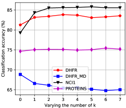
In this section, we test the performance of our graph kernel Tree++ on each real-world dataset when varying its two parameters, i.e., the depth $k$ of the truncated BFS tree in the super path, and the depth $d$ of the truncated BFS tree rooted at each vertex to extract path patterns. We vary the number of $k$ and $d$ both from zero to seven. When varying the number of $k$ , we fix $d=7$ . When varying the number of $d$ , we fix $k=1$ .

Figure 7 shows the classification accuracy of Tree++ on each real-world dataset when varying the number of $k$ . On the original chemical compound datasets, we can see that Tree++ tends to reach better classification accuracy with increasing values of $k$ . The tendency is reversed on the derived chemical compound datasets where explicit hydrogen atoms are removed. We can see from Figure 9 that compared with the original datasets BZR, COX2, and DHFR, the derived datasets BZR_MD, COX2_MD, and DHFR_MD have more diverse edge and degree distributions, i.e., the edge number and degree vary more than those of the original datasets. In addition, their degree distributions do not follow the power law. For graphs with many high degree vertices, the concatenation of vertex labels as a hash method for BFS trees in super paths can hurt the performance. For example, two BFS trees in super paths may just have one different vertex, which can lead to different hashing. Thus, with increasing values of $k$ , two graphs with many high degree vertices tend to be more dissimilar, which is a reason for the decreasing of classification accuracy in datasets BZR_MD, COX2_MD, and DHFR_MD. Since the degree distribution of the brain network dataset KKI follow the power law, we can observe a tendency of Tree++ to reach better classification accuracy with increasing values of $k$ . On all the molecular compound datasets whose degree distribution also follow the power law, we also observe a tendency of Tree++ to reach better classification accuracy with increasing values of $k$ . Another observation is that the classification accuracy of Tree++ first increase and then remain stable with increasing values of $k$ . One explaination is that if smaller values of $k$ can distinguish the structure identities of vertices, larger values of $k$ will not benefit much to the increase of classification accuracy.

Figure 8 shows the classification accuracy of Tree++ on each real-world dataset when varying the number of $d$ . On all the chemical compound datasets except COX2, and on all the molecular compound datasets and brain network dataset, Tree++ tends to become better with increasing values of $d$ . The phenomena are obvious because deep BFS trees can capture more path patterns around a vertex.

Refer to caption — Figure 7. The classification accuracy of Tree++ on each real-world dataset when varying the number of $k$ (the depth of the truncated BFS tree in the super path).

Table 2. Comparison of classification accuracy (

\pm

standard deviation) of Tree++ and its competitors on the real-world datasets.

Dataset	Tree++	MLG	DGK	RetGK	Propa	PM	SP	WL	FGSD
BZR	87.88 $\pm$ 1.00	86.28 $\pm$ 0.59	83.08 $\pm$ 0.53	86.30 $\pm$ 0.71	85.95 $\pm$ 0.85	82.35 $\pm$ 0.47	85.65 $\pm$ 1.02	87.25 $\pm$ 0.77	85.38 $\pm$ 0.85
BZR_MD	69.47 $\pm$ 1.14	48.87 $\pm$ 2.44	58.50 $\pm$ 1.52	62.77 $\pm$ 1.69	61.53 $\pm$ 1.27	68.20 $\pm$ 1.24	68.60 $\pm$ 1.94	59.67 $\pm$ 1.47	61.00 $\pm$ 1.35
COX2	84.28 $\pm$ 0.85	76.91 $\pm$ 1.14	78.30 $\pm$ 0.29	81.85 $\pm$ 0.83	81.33 $\pm$ 1.36	77.34 $\pm$ 0.82	80.87 $\pm$ 1.20	81.20 $\pm$ 1.05	78.30 $\pm$ 1.03
COX2_MD	69.20 $\pm$ 1.69	48.17 $\pm$ 2.43	51.57 $\pm$ 1.71	59.47 $\pm$ 1.66	55.33 $\pm$ 1.70	63.60 $\pm$ 0.87	65.70 $\pm$ 1.66	56.30 $\pm$ 1.55	48.97 $\pm$ 1.90
DHFR	83.68 $\pm$ 0.59	79.61 $\pm$ 0.50	64.13 $\pm$ 0.89	82.33 $\pm$ 0.66	80.67 $\pm$ 0.52	64.59 $\pm$ 1.25	77.80 $\pm$ 0.98	82.39 $\pm$ 0.90	78.13 $\pm$ 0.58
DHFR_MD	68.87 $\pm$ 0.91	67.87 $\pm$ 0.12	67.90 $\pm$ 0.26	64.44 $\pm$ 0.98	64.18 $\pm$ 0.97	66.21 $\pm$ 1.01	68.00 $\pm$ 0.36	64.00 $\pm$ 0.47	66.62 $\pm$ 0.78
NCI1	85.77 $\pm$ 0.12	78.20 $\pm$ 0.32	66.72 $\pm$ 0.29	84.28 $\pm$ 0.25	79.71 $\pm$ 0.39	63.55 $\pm$ 0.44	73.12 $\pm$ 0.29	84.79 $\pm$ 0.22	75.99 $\pm$ 0.51
PROTEINS	75.46 $\pm$ 0.47	72.01 $\pm$ 0.83	72.59 $\pm$ 0.51	75.77 $\pm$ 0.66	72.71 $\pm$ 0.83	73.66 $\pm$ 0.67	76.00 $\pm$ 0.29	75.32 $\pm$ 0.20	70.14 $\pm$ 0.67
Mutagenicity	83.64 $\pm$ 0.27	76.85 $\pm$ 0.38	66.80 $\pm$ 0.15	82.89 $\pm$ 0.18	81.47 $\pm$ 0.34	69.06 $\pm$ 0.14	77.52 $\pm$ 0.13	83.51 $\pm$ 0.27	70.71 $\pm$ 0.39
PTC_MM	68.03 $\pm$ 0.61	61.21 $\pm$ 1.08	67.09 $\pm$ 0.49	65.79 $\pm$ 1.76	64.12 $\pm$ 1.43	62.27 $\pm$ 1.51	62.18 $\pm$ 2.22	67.18 $\pm$ 1.61	57.88 $\pm$ 1.97
PTC_FR	68.71 $\pm$ 1.29	64.31 $\pm$ 2.00	67.66 $\pm$ 0.32	66.77 $\pm$ 0.99	65.14 $\pm$ 2.04	64.86 $\pm$ 0.88	66.91 $\pm$ 1.46	66.17 $\pm$ 1.02	63.80 $\pm$ 1.51
KKI	55.63 $\pm$ 1.69	48.00 $\pm$ 3.64	51.25 $\pm$ 4.17	48.50 $\pm$ 2.99	50.88 $\pm$ 4.17	52.25 $\pm$ 2.49	50.13 $\pm$ 3.46	50.38 $\pm$ 2.77	49.25 $\pm$ 4.76

5.2. Classification Results

Table 2 shows the classification accuracy of our graph kernel Tree++ and its competitors on the twelve real-world datasets. Tree++ is superior to all of the competitors on eleven real-world datasets. On the dataset COX2_MD, the classification accuracy of Tree++ has a gain of 5.3% over that of the second best method SP, and has a gain of 43.7% over that of the worst method MLG. On the dataset KKI, the classification accuracy of Tree++ has a gain of 6.5% over that of the second best method PM, and has a gain of 15.9% over that of the worst method MLG. On the datasets DHFR_MD, Mutagenicity, and PTC_MM, Tree++ is slightly better than WL. On the dataset PROTEINS, SP achieves the best classification accuracy. Tree++ achieves the second best classification accuracy. However, the classification accuracy of SP only has a gain of 0.7% over that of Tree++. To summarize, our Tree++ kernel achieves the highest accuracy on eleven datasets and is comparable to SP on the dataset PROTEINS.

Table 3. Comparison of runtime (in seconds) of Tree++ and its competitors on the real-world datasets.

Dataset	Tree++	MLG	DGK	RetGK	Propa	PM	SP	WL	FGSD
BZR	11.29	142.80	1.60	13.70	11.76	16.80	12.37	1.73	0.73
BZR_MD	4.73	89.93	1.23	4.22	4.89	17.15	17.81	7.72	0.07
COX2	14.57	78.29	2.26	15.73	7.28	6.48	4.81	0.92	0.14
COX2_MD	7.83	4.42	1.10	5.62	1.71	4.67	2.67	1.14	0.07
DHFR	26.24	200.05	4.44	48.95	14.17	16.01	12.07	1.95	0.22
DHFR_MD	8.10	19.03	1.12	10.02	3.01	6.82	4.65	1.49	0.08
NCI1	81.68	3315.42	39.35	761.45	221.84	326.43	22.89	101.68	1.39
PROTEINS	59.56	3332.31	48.83	49.07	27.72	32.79	36.38	38.66	0.49
Mutagenicity	87.09	4088.53	24.67	735.48	526.96	672.33	28.03	94.05	1.56
PTC_MM	1.99	152.69	1.08	2.84	2.44	10.00	1.83	0.95	0.08
PTC_FR	2.19	170.05	1.14	3.16	5.73	10.01	2.48	1.77	0.09
KKI	2.00	67.58	0.65	0.40	0.57	1.25	1.27	0.25	0.02

5.3. Runtime

Table 3 demonstrates the running time of every method on the real-world datasets. Tree++ scales up easily to graphs with thousands of vertices. On the dataset Mutagenicity, Tree++ finishes its computation in about one minute. It costs RetGK about twelve minutes to finish. It even costs MLG about one hour to finish. On the dataset NCI1, Tree++ finishes its computation in about one minute, while RetGK uses about twelve minutes and MLG uses about one hour. On the other datasets, Tree++ is comparable to SP and WL.

6. Discussion

Differing from the Weisfeiler-Lehman subtree kernel (WL) which uses subtrees (each vertex can appear repeatedly) to extract features from graphs, we use BFS trees to extract features from graphs. In this case, every vertex will appear only once in a BFS tree. Another different aspect is that we count the number of occurrences of each path pattern while WL counts the number of occurrences of each subtree pattern. If the BFS trees used in the construction of path patterns and super paths are of depth zero, Tree++ is equivalent to WL using subtree patterns of depth zero; If the BFS trees used in the construction of path patterns are of depth zero, and of super paths are of depth one, Tree++ is equivalent to WL using subtree patterns of depth one. In other cases, Tree++ and the Weisfeiler-Lehman subtree kernel deviate from each other. Tree++ is also related to the shortest-path graph kernel (SP) in the sense that both of them use the shortest paths in graphs. SP counts the number of pairs of shortest paths which have the same source and sink labels and the same length in two graphs. Each shortest-path used in SP is represented as a tuple in the form of “(source, sink, length)” which does not explicitly consider the intermediate vertices. However, Tree++ explicitly considers the intermediate vertices. If two shortest-paths with the same source and sink labels and the same length but with different intermediate vertices, SP cannot distinguish them whereas Tree++ can. Thus compared with SP, Tree++ has higher discrimination power.

As discussed in Section 1, WL can only capture the graph similarity at coarse granularities, and SP can only capture the graph similarity at fine granularities. By inheriting merits both from trees and shortest-paths, our method Tree++ can capture the graph similarity at multiple levels of granularities. Although MLG can also capture the graph similarity at multiple levels of granularities, it needs to invert the graph Laplacian matrix, which costs a lot of time. Tree++ is scalable to large graphs. Tree++ is built on the truncated BFS trees rooted at each vertex in a graph. One main problem is that the truncated BFS trees are not unique. To solve this problem, we build BFS trees considering the label and eigenvector centrality values of each vertex. Alternatively, we can also use other centrality metrics such as closeness centrality (Sabidussi, 1966) and betweenness centrality (Freeman, 1977) to order the vertices in the BFS trees. An interesting research topic in the future is to investigate the effects of using different centrality metrics to construct BFS trees on the performance of Tree++.

As stated in Section 2, hash functions have been integrated into the design of graph kernels. But they are just adopted for hashing continuous attributes to discrete ones. Conventionally, hash functions are developed for efficient nearest neighbor search in databases. Usually, people first construct a similarity graph from data and then learn a hash function to embed data points into a low-dimensional space where neighbors in the input space are mapped to similar codes (Liu et al., 2011). For two graphs, we can first use hash functions such as Spectral Hashing (SH) (Weiss et al., 2009) or graph embedding methods such as DeepWalk (Perozzi et al., 2014) to embed each vertex in a graph into a vector space. Each graph is represented as a set of vectors. Then, following RetGK (Zhang et al., 2018), we can use the Maximum Mean Discrepancy (MMD) (Gretton et al., 2012) to compute the similairty between two sets of vectors. Finally, we have a kernel matrix for graphs. This research direction is worth exploring in the future. Tree++ is designed for graphs with discrete vertex labels. Another research direction in the future is to extend Tree++ to graphs with both discrete and continuous attributes.

7. Conclusion

In this paper, we have presented two novel graph kernels: (1) The path-pattern graph kernel that uses the paths from the root to every other vertex in a truncated BFS tree as features to represent a graph; (2) The Tree++ graph kernel that incorporates a new concept of super path into the path-pattern graph kernel and can compare the graph similarity at multiple levels of granularities. Tree++ can capture topological relations between not only individual vertices, but also subgraphs, by adjusting the depths of truncated BFS trees in the super paths. Empirical studies demonstrate that Tree++ is superior to other well-known graph kernels in the literature regarding classification accuracy and runtime.

Acknowledgment

The authors would like to thank anonymous reviewers for their constructive and helpful comments. This work was supported partially by the National Science Foundation (grant # IIS-1817046) and by the U. S. Army Research Laboratory and the U. S. Army Research Office (grant # W911NF-15-1-0577).

References

(1)
Bonacich (1987) Phillip Bonacich. 1987. Power and centrality: A family of measures. American journal of sociology 92, 5 (1987), 1170–1182.
Borgwardt and Kriegel (2005) Karsten M Borgwardt and Hans-Peter Kriegel. 2005. Shortest-path kernels on graphs. In ICDM. IEEE, 8–pp.
Borgwardt et al. (2005) Karsten M Borgwardt, Cheng Soon Ong, Stefan Schönauer, SVN Vishwanathan, Alex J Smola, and Hans-Peter Kriegel. 2005. Protein function prediction via graph kernels. Bioinformatics 21, suppl_1 (2005), i47–i56.
Chang and Lin (2011) Chih-Chung Chang and Chih-Jen Lin. 2011. LIBSVM: a library for support vector machines. TIST 2, 3 (2011), 27.
Costa and Grave (2010) Fabrizio Costa and Kurt De Grave. 2010. Fast neighborhood subgraph pairwise distance kernel. In ICML. Omnipress, 255–262.
Debnath et al. (1991) Asim Kumar Debnath, Rosa L Lopez de Compadre, Gargi Debnath, Alan J Shusterman, and Corwin Hansch. 1991. Structure-activity relationship of mutagenic aromatic and heteroaromatic nitro compounds. correlation with molecular orbital energies and hydrophobicity. Journal of medicinal chemistry 34, 2 (1991), 786–797.
Feragen et al. (2013) Aasa Feragen, Niklas Kasenburg, Jens Petersen, Marleen de Bruijne, and Karsten Borgwardt. 2013. Scalable kernels for graphs with continuous attributes. In NIPS. 216–224.
Freeman (1977) Linton C Freeman. 1977. A set of measures of centrality based on betweenness. Sociometry (1977), 35–41.
Gärtner et al. (2003) Thomas Gärtner, Peter Flach, and Stefan Wrobel. 2003. On graph kernels: Hardness results and efficient alternatives. In Learning theory and kernel machines. Springer, 129–143.
Grauman and Darrell (2007) Kristen Grauman and Trevor Darrell. 2007. Approximate correspondences in high dimensions. In NIPS. 505–512.
Gretton et al. (2012) Arthur Gretton, Karsten M Borgwardt, Malte J Rasch, Bernhard Schölkopf, and Alexander Smola. 2012. A kernel two-sample test. JMLR 13, Mar (2012), 723–773.
Harary (1969) F Harary. 1969. Graph theory Addison-Wesley Reading MA USA.
Haussler (1999) David Haussler. 1999. Convolution kernels on discrete structures. Technical Report. Technical report, Department of Computer Science, University of California at Santa Cruz.
Horváth et al. (2004) Tamás Horváth, Thomas Gärtner, and Stefan Wrobel. 2004. Cyclic pattern kernels for predictive graph mining. In SIGKDD. ACM, 158–167.
Kashima et al. (2003) Hisashi Kashima, Koji Tsuda, and Akihiro Inokuchi. 2003. Marginalized kernels between labeled graphs. In ICML. 321–328.
Kondor and Pan (2016) Risi Kondor and Horace Pan. 2016. The multiscale laplacian graph kernel. In NIPS. 2990–2998.
Kong et al. (2011) Xiangnan Kong, Wei Fan, and Philip S Yu. 2011. Dual active feature and sample selection for graph classification. In SIGKDD. ACM, 654–662.
Kriege and Mutzel (2012) Nils Kriege and Petra Mutzel. 2012. Subgraph matching kernels for attributed graphs. arXiv preprint arXiv:1206.6483 (2012).
Kriege et al. (2016) Nils M Kriege, Pierre-Louis Giscard, and Richard Wilson. 2016. On valid optimal assignment kernels and applications to graph classification. In NIPS. 1623–1631.
Lee et al. (2018) John Boaz Lee, Ryan Rossi, and Xiangnan Kong. 2018. Graph classification using structural attention. In SIGKDD. ACM, 1666–1674.
Liu et al. (2011) Wei Liu, Jun Wang, Sanjiv Kumar, and Shih-Fu Chang. 2011. Hashing with graphs. (2011).
Mahé and Vert (2009) Pierre Mahé and Jean-Philippe Vert. 2009. Graph kernels based on tree patterns for molecules. Machine learning 75, 1 (2009), 3–35.
Morris et al. (2016) Christopher Morris, Nils M Kriege, Kristian Kersting, and Petra Mutzel. 2016. Faster kernels for graphs with continuous attributes via hashing. In ICDM. IEEE, 1095–1100.
Neumann et al. (2016) Marion Neumann, Roman Garnett, Christian Bauckhage, and Kristian Kersting. 2016. Propagation kernels: efficient graph kernels from propagated information. Machine Learning 102, 2 (2016), 209–245.
Neumann et al. (2012) Marion Neumann, Novi Patricia, Roman Garnett, and Kristian Kersting. 2012. Efficient graph kernels by randomization. In Joint European Conference on Machine Learning and Knowledge Discovery in Databases. Springer, 378–393.
Niepert et al. (2016) Mathias Niepert, Mohamed Ahmed, and Konstantin Kutzkov. 2016. Learning convolutional neural networks for graphs. In ICML. 2014–2023.
Nikolentzos et al. (2017) Giannis Nikolentzos, Polykarpos Meladianos, and Michalis Vazirgiannis. 2017. Matching node embeddings for graph similarity. In AAAI.
Orsini et al. (2015) Francesco Orsini, Paolo Frasconi, and Luc De Raedt. 2015. Graph invariant kernels. In Proceedings of the Twenty-fourth International Joint Conference on Artificial Intelligence. 3756–3762.
Pan et al. (2017) Shirui Pan, Jia Wu, Xingquan Zhu, Guodong Long, and Chengqi Zhang. 2017. Task sensitive feature exploration and learning for multitask graph classification. IEEE transactions on cybernetics 47, 3 (2017), 744–758.
Perozzi et al. (2014) Bryan Perozzi, Rami Al-Rfou, and Steven Skiena. 2014. Deepwalk: Online learning of social representations. In SIGKDD. ACM, 701–710.
Pržulj et al. (2004) Nataša Pržulj, Derek G Corneil, and Igor Jurisica. 2004. Modeling interactome: scale-free or geometric? Bioinformatics 20, 18 (2004), 3508–3515.
Ramon and Gärtner (2003) Jan Ramon and Thomas Gärtner. 2003. Expressivity versus efficiency of graph kernels. In Proceedings of the first international workshop on mining graphs, trees and sequences. 65–74.
Riesen and Bunke (2008) Kaspar Riesen and Horst Bunke. 2008. IAM graph database repository for graph based pattern recognition and machine learning. In SPR and SSPR. Springer, 287–297.
Sabidussi (1966) Gert Sabidussi. 1966. The centrality index of a graph. Psychometrika 31, 4 (1966), 581–603.
Shervashidze and Borgwardt (2009) Nino Shervashidze and Karsten M Borgwardt. 2009. Fast subtree kernels on graphs. In NIPS. 1660–1668.
Shervashidze et al. (2011) Nino Shervashidze, Pascal Schweitzer, Erik Jan van Leeuwen, Kurt Mehlhorn, and Karsten M Borgwardt. 2011. Weisfeiler-lehman graph kernels. JMLR 12, Sep (2011), 2539–2561.
Shervashidze et al. (2009) Nino Shervashidze, SVN Vishwanathan, Tobias Petri, Kurt Mehlhorn, and Karsten Borgwardt. 2009. Efficient graphlet kernels for large graph comparison. In Artificial Intelligence and Statistics. 488–495.
Siglidis et al. (2018) Giannis Siglidis, Giannis Nikolentzos, Stratis Limnios, Christos Giatsidis, Konstantinos Skianis, and Michalis Vazirgiannis. 2018. GraKeL: A Graph Kernel Library in Python. arXiv preprint arXiv:1806.02193 (2018).
Su et al. (2016) Yu Su, Fangqiu Han, Richard E Harang, and Xifeng Yan. 2016. A fast kernel for attributed graphs. In SDM. SIAM, 486–494.
Sutherland et al. (2003) Jeffrey J Sutherland, Lee A O’brien, and Donald F Weaver. 2003. Spline-fitting with a genetic algorithm: A method for developing classification structure- activity relationships. Journal of chemical information and computer sciences 43, 6 (2003), 1906–1915.
Tsitsulin et al. (2018) Anton Tsitsulin, Davide Mottin, Panagiotis Karras, Alex Bronstein, and Emmanuel Müller. 2018. NetLSD: Hearing the Shape of a Graph. (2018), 2347–2356.
Verma and Zhang (2017) Saurabh Verma and Zhi-Li Zhang. 2017. Hunt For The Unique, Stable, Sparse And Fast Feature Learning On Graphs. In NIPS. 88–98.
Vishwanathan et al. (2010) S Vichy N Vishwanathan, Nicol N Schraudolph, Risi Kondor, and Karsten M Borgwardt. 2010. Graph kernels. Journal of Machine Learning Research 11, Apr (2010), 1201–1242.
Wale et al. (2008) Nikil Wale, Ian A Watson, and George Karypis. 2008. Comparison of descriptor spaces for chemical compound retrieval and classification. Knowledge and Information Systems 14, 3 (2008), 347–375.
Weisfeiler and Lehman (1968) Boris Weisfeiler and AA Lehman. 1968. A reduction of a graph to a canonical form and an algebra arising during this reduction. Nauchno-Technicheskaya Informatsia 2, 9 (1968), 12–16.
Weiss et al. (2009) Yair Weiss, Antonio Torralba, and Rob Fergus. 2009. Spectral hashing. In NIPS. 1753–1760.
Yanardag and Vishwanathan (2015) Pinar Yanardag and SVN Vishwanathan. 2015. Deep graph kernels. In SIGKDD. ACM, 1365–1374.
Zhang et al. (2018) Zhen Zhang, Mianzhi Wang, Yijian Xiang, Yan Huang, and Arye Nehorai. 2018. RetGK: Graph Kernels based on Return Probabilities of Random Walks. In NIPS. 3964–3974.

Tree++: Truncated Tree Based Graph Kernels

Abstract.

1. Introduction

2. Related Work

3. The Model

3.1. Notations

3.2. The Path-Pattern Graph Kernel

Definition 0 (Path Pattern).

Theorem 2.

Proof.

3.3. Incorporating Structural Identity

Definition 0 (Super Path).

3.4. Tree++

Definition 0 (Graph Similarity at the kk-level of Granularity).

4. Experimental Setup

5. Experimental Results

5.1. Parameter Sensitivity

5.2. Classification Results

5.3. Runtime

6. Discussion

7. Conclusion

Acknowledgment

References

Definition 0 (Graph Similarity at the $k$ -level of Granularity).