Tree-Structured Data Clustering-Driven Neural Network for Intra Prediction in Video Coding
Abstract
As a crucial part of video compression, intra prediction utilizes local information of images to eliminate the redundancy in spatial domain. In both the High Efficiency Video Coding (H.265/HEVC) and Versatile Video Coding (H.266/VVC), multiple directional prediction modes are employed to find the texture trend of each block and then the prediction is made based on reference samples in the selected direction. Recently, the intra prediction schemes based on neural networks have achieved great success. In these methods, the networks are trained and applied to intra prediction to assist the directional prediction modes. In this paper, we propose a novel tree-structured data clustering-driven neural network (dubbed TreeNet) for intra prediction, which builds the networks and clusters the training data in a tree-structured manner. Specifically, in each network split and training process of TreeNet, every parent network on a leaf node is split into two child networks by adding or subtracting Gaussian random noise. Then a data clustering-driven training is applied to train the two derived child networks using the clustered training data of their parent. To test the performance, TreeNet is integrated into VVC and HEVC to combine with or replace the directional prediction modes. In addition, a fast termination strategy is proposed to accelerate the search of TreeNet. The experimental results demonstrate that TreeNet with the fast termination can reach an average of 2.8% Bjntegaard distortion rate (BD-rate) improvement (up to 8.1%) and 4.9% BD-rate improvement (up to 8.2%) over VVC (VTM-4.0) and HEVC (HM-16.9) with all intra configuration, respectively.
Index Terms:
Intra prediction, neural networks, network split, data clustering, tree structure.I Introduction
As the state of the art video coding standard, H.266/VVC [1] developed by the Joint Video Expert team (JVET) could achieve approximately 50% bitrate reduction for equivalent perceptual quality compared with its predecessor H.265/HEVC [2] [3] with computational complexity increase as a trade-off [4]. Especially, the bitrate saving provided by intra coding of VVC is 25.1% on average, and up to 29.3% over HEVC [5]. The improvement is mainly achieved by the more flexible block partition, the increased number of angular prediction modes, and additional advanced prediction techniques.
As a crucial part of intra prediction, the granularity of angular prediction modes can greatly influence the intra prediction performance. In HEVC, the number of angular prediction modes is 33. By adding a new mode between every two neighboring angular prediction modes of HEVC, the number of the angular prediction modes in VVC is increased to 65 for square blocks [5]. The increased angular prediction modes enable VVC to describe the directional patterns in local areas more precisely and thus give more reasonable prediction results.
Although more angular prediction modes can make intra prediction more accurate, it is still challenging to predict blocks with complex patterns, especially for blocks without obvious directional features. This is because the angular prediction modes in VVC and HEVC are all designed manually and almost equidistantly distributed with a certain direction. What’s more, for each mode, only a few reference pixels in a specific direction can be accessed and only simple linear interpolation is performed for prediction.
Recently, neural network-based video coding has been developed rapidly. For the hybrid video coding framework, deep tools are integrated into every single component [6], for example, intra prediction [7] -[14], inter prediction [15], [16], in-loop filtering [17] -[19], entropy coding [20], [21], and post-processing [22], [23]. For inter prediction, Yan et al. [15] proposed a fractional-pixel reference generation convolutional neural network (CNN) for both uni-directional and bi-directional motion compensation. To improve the bi-prediction performance, Zhao et al. [16] designed an enhanced bi-prediction scheme based on CNN to generate predicted blocks in a non-linear fashion to improve the coding performance. For in-loop filtering, neural networks either act as additional tools to improve the performance of filtering [17], [18], or replace the deblocking filter and the sample adaptive offset [19]. Neural networks could also be adopted as entropy coding tools to estimate the probabilities of predefined syntax elements, e.g., the quantized coefficient [20] and the transform index[21]. On the decoder side, neural network-based post-processing tools are applied to improve reconstruction quality [22], [23].
In the existing neural network-based intra predictions, the networks either directly generate the prediction pixels [7], [10] - [14] or enhance the prediction quality [8], [9] using available reference samples. In [7], block-context pairs are separated into two clusters according to a directional context-block relationship to train two neural networks individually. In [13], multiple network modes are trained and each corresponds to a certain range of direction prediction modes. In [10] - [12], more network modes (up to 35) are designed for blocks of different sizes, and the network architecture is further simplified. In [8] and [9], the well-trained CNNs are added after the intra prediction module to refine the prediction.
Motivated by the successful practice of progressively refined angular prediction modes in intra prediction, in this paper, a tree-structured data clustering-driven neural network (TreeNet) is proposed for intra prediction, which builds the networks and clusters the training data in a tree-structured manner rather than the parallel networks as in [7] and [10] - [13]. Specifically, in each network split and training process of TreeNet, every parent network on a leaf node is split into two child networks by adding or subtracting Gaussian random noise. Then a K-means-like [24] data clustering-driven training [17] is applied to train the two derived child networks using the clustered training data of their parent. In addition, a fast termination strategy is proposed to accelerate the search of TreeNet.
The main contributions of this work are summarized as follows:
1) A tree-structured data clustering-driven neural network (dubbed TreeNet) is proposed for intra prediction, which builds the networks and clusters the training data in a tree-structured manner. TreeNet is integrated into VVC and HEVC to combine with or replace the directional prediction modes.
2) A network split strategy is designed to split each parent network on a leaf node into two child networks by adding or subtracting Gaussian random noise. A data clustering-driven training is applied to train the two derived child networks using the clustered training data of their parent.
3) A fast termination strategy is proposed to accelerate the search of TreeNet.
The rest of the paper is organized as follows. Section II provides a brief overview of related works, including intra prediction in HEVC and VVC, and neural network-based intra predictions. The proposed TreeNet is detailed in Section III. In Section IV, the experimental results and more analyses are presented. Finally, the conclusion and future works are provided in Section V.
II Related Works
In this section, the intra predictions in HEVC and VVC are firstly presented. Then the related neural network-based intra predictions are reviewed.
II-A Intra Prediction in HEVC and VVC
In H.265/HEVC, the quadtree-based block partition is adopted for intra prediction and transformation [3]. Each picture is divided into disjunct square coding tree units (CTUs) of the same size, each of which serves as the root of a block partition quadtree structure. Along with the coding tree structure, the CTUs can be subdivided into coding units (CUs). A CU can be further split along the coding tree structure into smaller prediction units (PUs) and transform units (TUs). In VVC, the concepts of CU, PU, and TU are replaced by CU. A more advanced block partition mechanism with embedded multi-type trees (MTT), including quadtree (QT), binary tree (BT), and ternary tree (TT), is adopted [27].

In HEVC, there are 35 directional prediction modes as shown in Fig. 1, including planar mode, DC mode, and 33 angular prediction modes. Planar mode is designed for areas with gradually changing contents. DC mode aims to predict smooth textures, and the predicted sample values are populated with a constant value representing the average of all surrounding reference samples. Angular prediction modes are designed to model structures with directional edges. To better adapt to the diverse contents and different block sizes, the number of angular prediction modes is increased to 65 in VVC by adding a new mode between every two neighboring angular prediction modes of HEVC as shown in Fig. 1. What’s more, aiming at the problem of asymmetric distribution of direction prediction in the non-square block, VVC adopts wide angular intra prediction (WAIP) [28] in which 14 angles using prediction from the shorter side are replaced by more extreme angles using prediction from the longer side, bringing the total number of intra directions supported in VVC to 93.
In addition to the increased directional prediction modes, multiple additional advanced prediction techniques are designed in VVC to make better use of surrounding reference samples, such as matrix-based intra prediction (MIP) [11], position-dependent prediction combination (PDPC) [29], multiple reference lines (MRL) [30], and cross-component linear model (CCLM) [31]. In PDPC, filtering with spatially varying weights is applied to blocks that use Planar mode, DC mode, and certain angular prediction modes. To benefit the prediction for sharp content, MRL is designed to use the non-adjacent reference line which is one, two or four lines away from the current block for prediction rather than only using the nearest line as in traditional directional prediction. CCLM is designed for the prediction of chroma components. The chroma components can be predicted from the collocated reconstructed luma samples by linear models whose parameters are derived from adjacent reconstructed samples.
II-B Neural Network-Based Intra Prediction
Recently, neural network-based intra predictions in video coding have been developed rapidly and achieved impressive performance. In [7], a fully connected network-based intra prediction (IPFCN) is proposed to learn an end-to-end mapping from neighboring reconstructed pixels to the target block. The neural networks are fed by 8 reference lines above and on the left side of the target block. Two variants of IPFCN: IPFCN-S and IPFCN-D are designed. IPFCN-S has a single network that is trained utilizing an unclassified training data, while IPFCN-D has two networks that are trained by the data from the non-angular prediction modes (DC and Planar) and the other angular prediction modes separately. IPFCN-S and IPFCN-D could achieve 2.9% and 3.4% BD-rate improvement over HEVC, respectively.
In [10], different numbers of networks (up to 35) are designed for blocks of different sizes. All neural networks for a given block size share all layers but the last one. The network mode signaling is based on a sorted mode list, which is produced by another fully connected network. The bitrate saving in [10] is around 3.0% over HEVC. Compared with IPFCN, the network architecture is simplified. In a later version [11], each network has only one layer without non-linear activation, i.e. each network is reduced to a matrix plus a bias vector. Only one row and one column from the reconstructed picture are used as reference pixels, and only half of the pixels in the target block are generated by the selected network. The remaining half is generated by linear interpolation. This matrix-based intra prediction (MIP) has been adopted by VVC with a bitrate saving of 0.79% under all-intra configuration. In [13], multiple network modes (NM) are trained and each corresponds to a certain range of the directional prediction modes. A maximum 6.3% bitrate reduction is achieved by NM compared with HM-16.9 with 88 constraint. In [12], a novel training loss function that reflects properties of the residual quantization and coding stages is designed by applying the -norm and a sigmoid-function to the prediction residual in DCT domain. It could achieve a bitrate saving of 3.79% compared with VTM 1.0. Different from the fully connected structure applied in above-mentioned works, a progressive spatial recurrent neural network (PS-RNN) which consists of three spatial recurrent units is designed in [14], and the prediction is progressively generated by passing information from preceding contents to blocks to be encoded. PS-RNN achieves on average 2.7% bitrate reduction over HEVC.
Neural network could also be utilized for prediction result refinement. In [8], a convolutional neural network-based intra prediction is proposed. The block size is constrained as 88. After HEVC intra prediction, the target block, along with its three nearest reconstruction blocks, forms a 1616 block as the input of CNN. The output of the neural network is a residual block of the same size as the input. By subtracting the generated residual block from the original HEVC prediction result, the prediction quality can be enhanced. MSCNN proposed in [9] further improves this method by increasing the number of supported block sizes. In addition, the multi-scale feature extraction is proposed to take advantage of feature maps in different scales to improve the performance. MSCNN could achieve an average of 3.4% bitrate saving with all intra configuration over HEVC.
III The Framework of TreeNet
In this section, the network structure in TreeNet is first introduced. Then the construction of TreeNet and the data clustering-driven training are presented. After that, the fast termination strategy for the search of TreeNet is described. Finally, the details of how to integrate TreeNet into the VVC and HEVC are provided.
III-A Network Structure in TreeNet
The network structure in TreeNet is shown in Fig. 2 (a). The network is composed of four parts: the input layer, the output layer, the fully connected layers, and the non-linear activation layers. The network input is the reconstructed reference samples surrounding the target block. To utilize more spatial contextual information for more accurate prediction, the multi-reference-line scheme [32] is employed, thus the network input is a vector, where and are the width and height of the target block and is the number of reference lines. In TreeNet, . If some required reference pixels are not available, the vacancies are filled in by a padding mechanism which is similar to the method used in HEVC [33]. The network output is an vector, corresponding to the predicted pixels of the target block in raster order. Since overmuch non-square shapes are supported in VVC, we transform non-square shapes to square shapes as follows. Firstly, the shorter reference line is padded to the same length as the longer one. Then the prediction is obtained after cutting off the redundant part of the network output. The prediction of non-square blocks is shown in Figs. 2 (b) and (c).
All linear layers of the network in TreeNet are fully connected, which is convenient for the network split. Except for the last fully connected layer, all fully connected layers are with the same output dimension. In addition, except for the last fully connected layer, each fully connected layer is followed by a non-linear activation layer. If the depth of the neural network is represented by , the output of the layer can be calculated as follows:
| (1) |
where and represent the weights and bias, respectively. and are the input and output of the network. represents the non-linear activation function. In this paper, Parametric Rectified Linear Unit (PReLU) [34] is selected as the activation function.
In TreeNet, the number of reference lines is set as 8, and the network depth is set as 4, as recommended in [7]. Different networks are designed for square blocks of different sizes. The layer dimensions of networks are set to be 512, 1024, 1024, 2048, 2048 for 44, 88, 1616, 3232, and 6464 blocks,respectively.

III-B TreeNet Construction
In traditional Linde-Buzo-Gray (LBG) data clustering algorithm [35], a perturbation is produced and applied as an addition or subtraction term for splitting one clustering centroid into two. Inspired by [35], we design a network split method for TreeNet. In each network split, every parent network on a leaf node is split into two networks by adding or subtracting Gaussian random noise to its each layer. The variance of the introduced Gaussian random noise is decided by the weights of each layer so that the mapping from the input to the output in the subsequent activation function won’t be changed. The two derived child networks have the same structure as their parent network. Fig. 3 (a) is an example of splitting one parent network into two child networks, where represents the Gaussian random noise introduced to the layer.

The networks in TreeNet are built in a tree-structured manner. An example of constructing TreeNet with =4 is shown in Fig. 3 (b). TreeNet is a perfect binary tree network and the number of networks at level is . The total number of networks in TreeNet with = is . After each network split, a data clustering-driven training is applied to train the every two derived child networks using the clustered training data of their parent.
As TreeNet goes deeper, the encoder complexity and memory burden will increase exponentially, and the overhead to indicate the networks will also increase. If the network split can’t bring enough prediction improvement, the network split will be terminated.
III-C Data Clustering-Driven Training of TreeNet
Inspired by the K-means-like training strategy in [17], a data clustering-driven training is applied to train every two derived child networks using the clustered training data of their parent. Fig. 4 is an example of the data clustering and the network training.
1) Clustering and Training: In each iteration of clustering and training, the training data of a parent network is first clustered according to the recovery qualities of the two derived child networks. In this paper, the squared error between original pixels and the prediction is used to measure the recovery quality. Then the clustered training data are fed into the corresponding derived child networks for training. Given a collection of training sample pairs, the loss function is formulated as:
| (2) |
where represents the network output and represents the ground truth. is the parameter set. represents the weight of the regularization term, and it is set to be in the experiments. is the weight of fully connected layers. The optimization algorithm to update all parameters is the stochastic gradient descent () with a momentum term [36]. The momentum of is set as 0.9.
After several iterations of clustering and training, the training loss gradually converges, which indicates that the clustering centers no longer move. Then the data clustering-driven training will stop.
2) Training Details: Firstly, the parameter set is initialized. The weight is randomly generated from a Gaussian distribution with a mean of 0 and a standard deviation of 1. The bias is initialized as 0. The scale factor in PReLU layers is initialized as 0.25. Then a root network of TreeNet is pre-trained for 80 epochs. The base learning rate is set to 0.1 as recommended in [7] and [9]. The network is trained with a fixed learning rate for 20 epochs and then uses the exponentially decaying learning for another 20 epochs until its convergence. The child networks are trained with exponentially decaying learning rates from 0.01 to 0.00001 for 40 epochs. The learning rate settings are listed in Table I.

| Num of Epochs | Learning Rate | Step | |
|---|---|---|---|
| Pre-train | 80 | 0.1-0.0001 | 20 |
| Recursive train | 40 | 0.01-0.00001 | 10 |
III-D Fast Termination Strategy
After TreeNet is well-trained, it can be used for intra prediction. However, the full search of TreeNet is very time consuming. Since the training of derived child networks only use the clustered training data from their parent network, the predictions between a parent network and its two child networks are correlated. Therefore, a fast termination strategy for TreeNet is proposed by exploring the correlation, which is shown in Algorithm 1. The rate-distortion (R-D) cost of a network can be expressed as:
| (3) |
where , , and represent the R-D cost, the sum of squared error (SSE), and costed bits, respectively. is the Lagrange multiplier decided by a quantization parameter (QP). The R-D cost difference between a child network and its parent network can be calculated as:
| (4) |
where the subscripts: and represent the child network and the parent network. If and are not smaller than 0, indicating that the parent network is better than both the two derived child networks, the search of TreeNet will be early terminated. Otherwise, the derived child network with less R-D cost will be searched, while the other child network is ignored. The fast termination strategy could help save the encoding running time greatly because at most networks are searched in TreeNet with = compared with networks for the full search.
III-E Integrating TreeNet in VVC and HEVC
To test the performance of TreeNet, we integrate TreeNet into VVC and HEVC reference softwares. In VVC, the best prediction mode is decided at the CU level. Fig. 5 shows an example of integrating TreeNet into the VVC framework. RDO means the rate-distortion optimization [37]. Similar to MRL, TreeNet doesn’t work with Intra Sub-Partitions (ISP) coding mode [38]. A new flag has to be coded and transmitted in the bitstream to indicate whether TreeNet is used or not. In HEVC, the best prediction mode is decided at the PU level. The integration of TreeNet in HEVC is exactly the same as in VVC.

| Level | Mode | Binarization | |||||
| 1 | 1 | 0 | |||||
| 2 | 2 | 1 | 0 | 0 | |||
| 3 | 1 | 1 | 0 | ||||
| 3 | 4 | 1 | 0 | 1 | 0 | 0 | |
| 5 | 1 | 0 | 1 | 1 | 0 | ||
| 6 | 1 | 1 | 1 | 0 | 0 | ||
| 7 | 1 | 1 | 1 | 1 | 0 | ||
| 4 | 8 | 1 | 0 | 1 | 0 | 1 | 0 |
| 9 | 1 | 0 | 1 | 0 | 1 | 1 | |
| 10 | 1 | 0 | 1 | 1 | 1 | 0 | |
| 11 | 1 | 0 | 1 | 1 | 1 | 1 | |
| 12 | 1 | 1 | 1 | 0 | 1 | 0 | |
| 13 | 1 | 1 | 1 | 0 | 1 | 1 | |
| 14 | 1 | 1 | 1 | 1 | 1 | 0 | |
| 15 | 1 | 1 | 1 | 1 | 1 | 1 | |
The codeword of each TreeNet mode is shown in Table. II. At each branch, one bit is needed to represent if the parent network is better than child networks, which is indicated by . If a child network works better, another bit is needed to represent which child network is better, which is indicated by . Therefore, 1, 3, 5, and 6 bits are needed for coding TreeNet modes at level , , , and , respectively. The Context-Based Adaptive Binary Arithmetic Coding (CABAC) [39] is used to encode the codewords and a context model is built for a corresponding bit.
IV Experiment Results
In this section, the experiment results of TreeNet are presented and analyzed in detail. Firstly, we introduce the experiment setting briefly. Secondly, the training dataset is presented. Thirdly, the overall performance of TreeNet integrated into VVC and HEVC is presented, respectively. After that, the usage rate, model size, and memory cost are provided. Finally, the data clustering-driven training is investigated.
IV-A Experiment Setting
To test the performance of TreeNet, it is implemented into VVC reference software VTM-4.0 and HEVC reference software HM-16.9. Libtorch is used to perform the feed-forward of networks. All experiments comply with the common test conditions specified in [40] and [41] with QP set as 22, 27, 32, 37, and the all-intra main configuration is deployed. 24 video sequences with different resolutions, grouped as , , , , and , are utilized for experiments, and the first frame of each sequence is tested. Bjntegaard distortion rate (BD-rate) [42] is used to evaluate the performance.
In our experiments, TreeNet is trained using the deep learning framework Pytorch [44] 1.8.0 on NVIDIA GeForce RTX 3060 GPU. The models for small blocks (44 and 88) are trained with a batch size of 512, while the models for large blocks (1616 to 6464) are trained with a batch size of 256.
IV-B Training Dataset
The training data is generated from pictures in the New York city library image set [43]. Firstly, these images are converted to YUV 4:2:0 color format. Then all training images are encoded with all intra configuration. The QP is set to 22, 27, 32, and 37. For all QPs, the encoder generates 5 different bitstreams for different block sizes from 44 to 6464 separately, which will be used to train the models in TreeNet for different block sizes. The reconstructed reference samples of a block are extracted from the bitstreams on the decoder side as the network input. The original pixels of the block are taken as the ground truth.
It should be noted that, before the recursive training, all training data should be pre-processed by zero-centering to get rid of the low-frequency component and make the training easier. In [7] and [9], blocks with complex textures are excluded from the training data since such data would degrade the training efficiency and practical performance, while in TreeNet training, all blocks are kept in the training data.
| Sequence | TreeNet | Fast TreeNet | MIP [11] | ||||
| Depth=1 | Depth=2 | Depth=3 | Depth=4 | Depth=3 | - | ||
| Class A (4K) | Tango2 | -4.4% | -5.5% | -6.2% | -6.3% | -6.0% | -1.5% |
| FoodMarket4 | -6.2% | -7.8% | -8.3% | -8.5% | -8.1% | -1.3% | |
| Campfire | -1.9% | -2.4% | -2.7% | -2.8% | -2.6% | -0.7% | |
| CatRobot | -1.8% | -2.6% | -3.0% | -3.1% | -2.9% | -0.7% | |
| DaylightRoad2 | -2.0% | -2.7% | -3.0% | -3.0% | -2.9% | -0.6% | |
| ParkRunning3 | -1.3% | -1.7% | -2.2% | -2.4% | -2.0% | -0.6% | |
| Class B (1080P) | MarketPlace | -1.8% | -2.3% | -2.7% | -2.7% | -2.7% | -0.7% |
| RitualDance | -2.7% | -3.3% | -3.7% | -3.8% | -3.6% | -1.0% | |
| Kimono | -1.6% | -2.3% | -2.6% | -2.8% | -2.6% | - | |
| ParkScene | -1.4% | -2.0% | -2.4% | -2.4% | -2.3% | - | |
| Cactus | -1.4% | -2.0% | -2.5% | -2.6% | -2.3% | -0.7% | |
| BasketballDrive | -1.9% | -2.2% | -2.5% | -2.6% | -2.4% | -0.6% | |
| BQTerrace | -1.2% | -1.6% | -2.0% | -1.9% | -2.0% | -0.4% | |
| Class C (WVGA) | BasketballDrill | -1.0% | -1.3% | -1.7% | -1.6% | -1.6% | -0.7% |
| BQMall | -1.4% | -1.8% | -2.1% | -2.2% | -2.0% | -0.8% | |
| PartyScene | -1.3% | -1.7% | -2.0% | -2.0% | -1.9% | -0.7% | |
| RaceHorses | -1.6% | -2.0% | -2.2% | -2.3% | -2.2% | -0.7% | |
| Class D (WQVGA) | BasketballPass | -1.2% | -1.3% | -1.6% | -1.6% | -1.5% | -0.8% |
| BQSquare | -0.8% | -1.2% | -1.5% | -1.5% | -1.5% | -0.8% | |
| BlowingBubbles | -1.6% | -1.7% | -1.9% | -1.9% | -1.7% | -0.7% | |
| RaceHorses | -1.9% | -2.4% | -2.7% | -2.7% | -2.6% | -0.9% | |
| Class E (720P) | FourPeople | -2.0% | -2.6% | -3.0% | -3.0% | -2.9% | -0.8% |
| Johnny | -2.4% | -2.7% | -3.2% | -3.0% | -3.0% | -0.9% | |
| KristenAndSara | -1.6% | -2.2% | -2.7% | -2.7% | -2.6% | -0.8% | |
| Average | -1.9% | -2.5% | -2.9% | -2.9% | -2.8% | -0.8% | |
IV-C Comparison with H.266/VVC
In the experiments, we first test the performance of applying TreeNet with different depths to the VTM-4.0. Then the performance of the fast termination strategy is provided.
The experimental results are shown in Table III. As observed, TreeNet with =4, 3, 2, and 1 can bring an average BD-rate saving of 2.9%, 2.9%, 2.5%, and 1.9% for the luma component, respectively. For all test sequences, TreeNet with =4 brings similar gains as TreeNet with =3. Therefore, TreeNet with =3 is adopted and used in the following experiments. For simplicity, we call TreeNet with =3 as TreeNet in the following. The performance of TreeNet with the fast termination strategy (fast TreeNet) is degraded to an average of 2.8% BD-rate saving (up to 8.1%), however the encoding time is much reduced, which is shown in Table IV. Compared with MIP [11], which has simpler network architecture and more network modes than TreeNet, the BD-rate improvement brought by TreeNet is significant, reaching 2.0% improvement on average.
| Anchor | Depth | Encoding Time | Decoding Time | |
| VTM | TreeNet | 1 | 753% | 3909% |
| 2 | 1872% | 4613% | ||
| 3 | 4115% | 5173% | ||
| 4 | 8632% | 5294% | ||
| Fast TreeNet | 3 | 2493% | 5061% | |
| MIP [11] | - | 138% | 99% | |
-
*
Anchor is 100%
The running times of these tests are summarized in Table IV. All tests for TreeNet are done with an AMD Ryzen7 5800H CPU and an NVIDIA GeForce RTX 3060 GPU. MIP is conducted on an Intel Xeon cluster (E5-2697A v4). As TreeNet goes deeper, the encoding time increases exponentially. The encoding time of TreeNet with =3 is around 41 times of the anchor. With the fast termination strategy, the encoding time is reduced to around 25 times. The decoding time of fast TreeNet is roughly 50 times of the anchor. Compared with MIP, both the encoding and decoding time increase greatly due to the complex network structure in TreeNet. How to simplify the network structure in TreeNet is our future work.
In addition to the BD-rate saving, we also provide some visual examples of prediction results of TreeNet and compare them with VVC intra prediction. The examples are taken from the first frame of Kimono encoded with QP=27. The comparison results are shown in Figs. 6, 7, and 8. As observed, TreeNet could produce more accurate predictions than the VVC directional prediction modes. As shown in Fig. 6, the prediction of TreeNet distinguishes the black and white areas more accurately and clearly than the directional prediction of VVC. In Fig. 7, TreeNet generates the predictions that are closer to the original textures compared with the VVC intra prediction. In Fig. 8, there is an obvious directional pattern in the original block. TreeNet could still generate better predictions than the VVC directional prediction mode.


| Sequence | HM | HM with 8x8 constraint | ||||||
| Fast TreeNet | IPFCN-D[7] | PS-RNN[14] | Fast TreeNet | NM[13] | IPFCN-D[7] | PS-RNN[14] | ||
| Class A (4K) | Tango | -8.2% | -7.4% | - | -20.1% | -18.4% | -15.6% | - |
| Drums | -4.4% | -3.8% | - | -8.6% | -6.7% | -2.5% | - | |
| CampfireParty | -4.3% | -3.0% | - | -6.4% | -7.7% | -4.3% | - | |
| ToddlerFountain | -4.4% | -3.4% | - | -5.8% | -5.7% | -3.1% | - | |
| CatRobot | -6.0% | -4.2% | - | -9.7% | -8.0% | -5.7% | - | |
| TrafficFlow | -6.5% | -4.2% | - | -12.7% | -8.4% | -7.2% | - | |
| DaylightRoad | -6.4% | -4.5% | - | -8.4% | -8.5% | -7.0% | - | |
| Rollercoaster | -5.9% | -5.8% | - | -18.9% | -17.8% | -11.6% | - | |
| Class B 1080P | Kimono | -4.6% | -3.1% | -2.2% | -14.9% | -10.9% | -5.5% | -6.6% |
| ParkScene | -4.8% | -3.6% | -2.8% | -4.9% | -4.4% | -2.3% | -3.4% | |
| Cactus | -4.6% | -3.2% | -2.5% | -5.8% | -4.3% | -2.0% | -3.3% | |
| BasketballDrive | -5.4% | -3.6% | -1.8% | -11.6% | -9.9% | -4.6% | -7.8% | |
| BQTerrace | -3.8% | -2.1% | -2.6% | -3.7% | -3.2% | -1.6% | -2.6% | |
| Class C (WVGA) | BasketballDrill | -2.9% | -1.5% | -2.1% | -2.9% | -1.6% | 1.2% | -2.9% |
| BQMall | -4.0% | -2.2% | -3.1% | -3.6% | -3.5% | -1.4% | -2.9% | |
| PartyScene | -3.0% | -1.6% | -2.6% | -2.9% | -2.4% | -1.1% | -2.3% | |
| RaceHorsesC | -3.5% | -3.2% | -1.4% | -4.1% | -3.1% | -1.2% | -2.8% | |
| Class D (WQVGA) | BasketballPass | -3.6% | -1.2% | -1.8% | -3.0% | -2.7% | 0.4% | -2.5% |
| BQSquare | -2.7% | -0.9% | -2.0% | -1.5% | -1.6% | -0.8% | -1.8% | |
| BlowingBubbles | -3.2% | -1.9% | -2.8% | -3.1% | -2.7% | -1.3% | -2.3% | |
| RaceHorses | -4.8% | -3.2% | -3.5% | -4.0% | -3.1% | -1.0% | -2.6% | |
| Class E (720P) | FourPeople | -6.6% | -4.4% | -3.8% | -6.9% | -6.0% | -3.4% | -6.8% |
| Johnny | -7.2% | -5.3% | -4.0% | -9.5% | -8.6% | -8.3% | -5.6% | |
| KristenAndSara | -5.8% | -3.9% | -3.2% | -7.6% | -6.7% | -5.8% | -6.6% | |
| Average | -4.9% | -3.4% | -2.7% | -7.5% | -6.5% | -4.0% | -3.9% | |
IV-D Comparison with H.265/HEVC and The State of The Art
We compare fast TreeNet with Intra Prediction Fully-Connected Networks (IPFCN) [7], Progressive Spatial Recurrent Neural Network (PS-RNN) [14], and multiple neural network model-based enhanced intra prediction (NM) [13]. Among these approaches, NM in [13] only allows 88 intra coding, and such a manner is also applied in PS-RNN. In [13], IPFCN-D integrated into HM with 88 constraint is also reimplemented. To make a more detailed comparison, fast TreeNet is implemented with and without 88 constraint, respectively. The comparison results are presented in Table V.
As shown in Table V, for the luma component, fast TreeNet brings an average BD-rate saving of 4.9% (up to 8.2%). Compared with IPFCN-D, fast TreeNet achieves 1.5% BD-rate reduction on average. Fast TreeNet can also bring an average of 1.7% BD-rate reduction over PS-RNN on Class B, C, D, and E. When only 88 intra coding is allowed, the improvement of fast TreeNet is more obvious, reaching an average of 7.5% BD-rate reduction. Compared with IPFCN-D and NM, fast TreeNet achieves 3.5% and 1.0% BD-rate reduction on average, respectively. Fast TreeNet can also bring 1.7% BD-rate reduction on average over PS-RNN on Class B, C, D, and E.
Furthermore, we replace all the directional prediction modes in HEVC with fast TreeNet and test the performance on the first frame of some high-resolution sequences. The results are presented in Table VI. As shown in Table VI, fast TreeNet with =4 and 3 brings an average of 2.3% and 2.1% BD-rate reduction respectively, which indicates fast TreeNet replacing all the directional prediction modes still performs well for high-resolution sequences. The result also indicates that more networks should be adopted when TreeNet is used to replace the directional prediction modes than combining with them.
| Sequence | Fast TreeNet | ||
| Depth=3 | Depth=4 | ||
| Class A (4K) | Tango | -4.8% | -5.0% |
| Drums | -1.6% | -1.9% | |
| CampfireParty | -1.2% | -1.4% | |
| ToddlerFountain | -3.0% | -3.2% | |
| CatRobot | -1.4% | -1.6% | |
| TrafficFlow | -1.5% | -1.6% | |
| FaylightRoad | -2.7% | -3.1% | |
| Rollercoaster | -1.9% | -2.2% | |
| Traffic | -2.9% | -3.1% | |
| PeopleOnStreet | -3.4% | -3.4% | |
| Class B (1080P) | Kimono | -2.5% | -2.8% |
| ParkScene | -2.6% | -2.9% | |
| Cactus | -0.8% | -1.2% | |
| BasketballDrive | -0.9% | -1.1% | |
| BQTerrace | -0.2% | -0.3% | |
| Average | -2.1% | -2.3% | |
IV-E Usage Rate
We calculate the usage rate of fast TreeNet at the pixel level when combining with the VVC directional prediction modes, which can be calculated by:
| (5) |
where denotes the usage rate. and denote the width and height of each frame. represents the number of blocks with a size of coded by fast TreeNet in each frame. Since MTT [27] is enabled in VTM, there are 14 blocks sizes supported. The QPs are set as . As shown in Table VII, the usage rates of fast TreeNet in all sequences are remarkable, especially in Class A. The average usage rate of fast TreeNet in all test sequences is 51.3% (up to 71.7%), which demonstrates its efficiency.
Furthermore, we provide an example of the usage rates of fast TreeNet at different levels for different block sizes, which is shown in Fig. 9. We can observe that fast TreeNet has a significant usage rate in predicting blocks of all sizes. For blocks of size 44, 48, 84, and 88, the usage rates of fast TreeNet are more than 80%, which demonstrates that fast TreeNet has more advantage in predicting small blocks than the directional prediction modes.
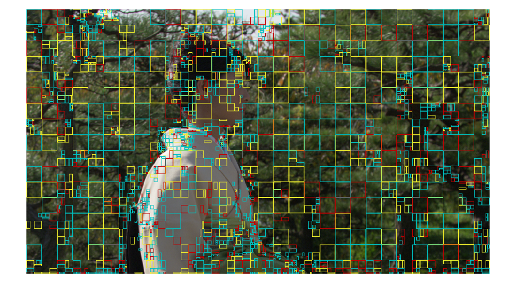
The visual result is shown in Fig. 10. The background parts, such as the tree leaves, are mostly coded by fast TreeNet with large blocks. The foreground parts and background parts with sharp edges, such as the woman’s head, the belt, and the trunks, are mostly coded by fast TreeNet with small blocks.

| Sequence | Usage Rate | |
|---|---|---|
| Class A (4K) | Tango2 | 71.1% |
| FoodMarket4 | 71.7% | |
| Campfire | 61.8% | |
| CatRobot | 48.4% | |
| DaylightRoad2 | 51.1% | |
| ParkRunning3 | 58.0% | |
| Class B (1080P) | MarketPlace | 54.3% |
| RitualDance | 53.4% | |
| Kimono | 70.5% | |
| ParkScene | 51.3% | |
| Cactus | 46.1% | |
| BasketballDrive | 44.4% | |
| BQTerrace | 39.6% | |
| ClassC (WVGA) | BasketballDrill | 38.5% |
| BQMall | 44.6% | |
| PartyScene | 49.7% | |
| RaceHorses | 52.3% | |
| ClassD (WQVGA) | BasketballPass | 38.7% |
| BQSquare | 38.3% | |
| BlowingBubbles | 51.8% | |
| RaceHorses | 53.6% | |
| Class E (720P) | FourPeople | 46.1% |
| Johnny | 50.9% | |
| KristenAndSara | 45.4% | |
| Average | 51.3% | |
| 64x64 | 32x32 | 16x16 | 8x8 | 4x4 | |
| Model Size | 80.5MB | 48.5MB | 11.2MB | 9.5MB | 2.4 MB |
IV-F Model Size and Memory Cost
The size of each Libtorch model in TreeNet is listed in Table VIII. The model size for block of 6464, 3232, 1616, 88, and 44 are 80.5 MB, 48.5 MB, 11.2 MB, 9.5 MB, and 2.4 MB respectively. There are 7 models for each block size in TreeNet, so overall MB is needed to store TreeNet with =3 in memory. In addition, another KB should be allocated in memory to store the 8-line reference samples.
| Level 2 | Iteration | 2 | 3 | ||||||
|---|---|---|---|---|---|---|---|---|---|
| 1 | 124.53 | 126.16 | |||||||
| 2 | 113.82 | 116.51 | |||||||
| 3 | 109.93 | 113.74 | |||||||
| 4 | 108.13 | 112.27 | |||||||
| 5 | 107.23 | 111.39 | |||||||
| 6 | 106.85 | 110.66 | |||||||
| 7 | 106.50 | 110.31 | |||||||
| 8 | 105.70 | 109.95 | |||||||
| Level 3 | Iteration | 4 | 5 | 6 | 7 | ||||
| 1 | 101.56 | 90.80 | 103.68 | 98.84 | |||||
| 2 | 99.52 | 85.20 | 102.26 | 92.23 | |||||
| 3 | 100.11 | 82.73 | 101.97 | 89.52 | |||||
| 4 | 101.02 | 81.27 | 102.55 | 88.07 | |||||
| 5 | 102.82 | 79.89 | 102.63 | 87.13 | |||||
| 6 | 104.15 | 78.93 | 102.91 | 86.51 | |||||
| 7 | 105.73 | 77.97 | 103.68 | 85.39 | |||||
| 8 | 105.96 | 77.11 | 103.94 | 85.02 | |||||
| Level 4 | Iteration | 8 | 9 | 10 | 11 | 12 | 13 | 14 | 15 |
| 1 | 96.55 | 97.73 | 72.47 | 69.42 | 93.90 | 95.52 | 78.45 | 77.08 | |
| 2 | 94.01 | 91.95 | 70.47 | 66.49 | 88.91 | 92.71 | 75.47 | 73.65 | |
| 3 | 94.38 | 88.36 | 70.01 | 64.62 | 86.50 | 92.45 | 74.48 | 72.49 | |
| 4 | 95.41 | 85.34 | 70.63 | 63.83 | 84.96 | 92.23 | 74.19 | 72.14 | |
| 5 | 96.53 | 83.76 | 70.33 | 63.16 | 83.77 | 92.66 | 73.53 | 71.87 | |
| 6 | 98.57 | 81.44 | 70.54 | 62.61 | 82.65 | 92.76 | 73.15 | 71.39 | |
| 7 | 100.10 | 80.21 | 70.40 | 62.00 | 82.17 | 92.95 | 72.92 | 71.50 | |
| 8 | 101.03 | 78.37 | 70.88 | 61.57 | 81.47 | 93.04 | 72.47 | 71.53 | |
| Level 2 | Iteration | 2 | 3 | ||||||
|---|---|---|---|---|---|---|---|---|---|
| 1-2 | 0.798 | 0.793 | |||||||
| 2-3 | 0.914 | 0.911 | |||||||
| 3-4 | 0.942 | 0.944 | |||||||
| 4-5 | 0.956 | 0.957 | |||||||
| 5-6 | 0.965 | 0.969 | |||||||
| 6-7 | 0.973 | 0.970 | |||||||
| 7-8 | 0.977 | 0.974 | |||||||
| Ratio | 50.3% | 49.7% | |||||||
| Level 3 | Iteration | 4 | 5 | 6 | 7 | ||||
| 1-2 | 0.783 | 0.848 | 0.786 | 0.821 | |||||
| 2-3 | 0.886 | 0.941 | 0.900 | 0.925 | |||||
| 3-4 | 0.916 | 0.966 | 0.933 | 0.950 | |||||
| 4-5 | 0.928 | 0.976 | 0.946 | 0.962 | |||||
| 5-6 | 0.942 | 0.981 | 0.956 | 0.969 | |||||
| 6-7 | 0.945 | 0.984 | 0.956 | 0.971 | |||||
| 7-8 | 0.952 | 0.985 | 0.962 | 0.974 | |||||
| Ratio | 18.6% | 31.7% | 22.2% | 27.5% | |||||
| Level 4 | Iteration | 8 | 9 | 10 | 11 | 12 | 13 | 14 | 15 |
| 1-2 | 0.821 | 0.834 | 0.804 | 0.822 | 0.822 | 0.805 | 0.802 | 0.813 | |
| 2-3 | 0.914 | 0.938 | 0.906 | 0.924 | 0.926 | 0.907 | 0.918 | 0.925 | |
| 3-4 | 0.934 | 0.964 | 0.936 | 0.951 | 0.950 | 0.937 | 0.949 | 0.951 | |
| 4-5 | 0.944 | 0.973 | 0.951 | 0.961 | 0.963 | 0.946 | 0.959 | 0.963 | |
| 5-6 | 0.947 | 0.978 | 0.957 | 0.969 | 0.967 | 0.958 | 0.966 | 0.966 | |
| 6-7 | 0.950 | 0.982 | 0.961 | 0.972 | 0.972 | 0.962 | 0.968 | 0.970 | |
| 7-8 | 0.954 | 0.983 | 0.963 | 0.974 | 0.976 | 0.963 | 0.972 | 0.970 | |
| Ratio | 7.9% | 10.7% | 14.7% | 17.0% | 12.0% | 10.2% | 13.5% | 14.0% | |
IV-G Investigations on The Data Clustering-Driven Training
To assess the data clustering-driven training, we first give some investigations on the prediction losses during the network split and iterative training. The average training losses of each network mode at level , , and in TreeNet for 88 blocks are provided in Tables IX. The average training losses of TreeNet modes gradually decrease and converge during the iterative data clustering-driven training. Then we conduct a statistic of the rate of samples remaining in the same cluster after each round of data clustering to see whether the data clustering could finally converge as shown in Table X. In addition, the ratio of the training data to the entire training dataset after the last iteration is also provided. We can observe that less and less training data is clustered to another cluster during the iterative training, which indicates that the data clustering and network training are gradually stabilized.
V Conclusions
In this paper, a novel tree-structured data clustering-driven neural network for intra prediction is proposed which builds the networks and clusters the training data in a tree-structured manner. Specifically, in each network split and training process of TreeNet, each parent network on a leaf node is split into two child networks by adding or subtracting Gaussian random noise. Then a data clustering-driven training is applied to train the two derived child networks. In addition, a fast termination strategy is proposed to accelerate the search of TreeNet. TreeNet could be applied to combine with or replace the directional prediction modes. Although TreeNet has been implemented into HEVC (HM-16.9) and VVC (VTM-4.0) and shows advantages, its network structure is too complex for practical applications. In future, we will focus its simplification like MIP in VVC and study to replace the directional prediction modes in VVC.
References
- [1] Versatile Video Coding, document ITU-T Rec. H.266 and ISO/IEC 23090-3, ITU-T and ISO/IEC, 2020.
- [2] High Efficiency Video Coding, document ITU-T Rec. H.265 and ISO/IEC 23008-2, vers. 1, ITU-T and ISO/IEC, 2013.
- [3] G. J. Sullivan, J. R. Ohm, W. J. Han, and T. Wiegand, “Overview of the high efficiency video coding (HEVC) standard,” IEEE Transactions on Circuits and Systems for Video Technology, vol. 22, no. 12, pp. 1649–1668, Dec 2012.
- [4] B. Bross et al., “Overview of the Versatile Video Coding (VVC) Standard and its Applications,” IEEE Transactions on Circuits and Systems for Video Technology, vol. 31, no. 10, pp. 3736-3764, Oct 2021.
- [5] J. Pfaff et al., “Intra Prediction and Mode Coding in VVC,” IEEE Transactions on Circuits and Systems for Video Technology, vol. 31, no. 10, pp. 3834-3847, Oct 2021.
- [6] D. Liu, Z. Chen, S. Liu and F. Wu, “Deep learning-based technology in responses to the joint call for proposals on video compression with capability beyond HEVC,” IEEE Transactions on Circuits and Systems for Video Technology, vol. 30, no. 5, pp. 1267-1280, May 2020.
- [7] J. Li, B. Li, J. Xu, R. Xiong, and W. Gao, “Fully connected networkbased intra prediction for image coding,” IEEE Transactions on Image Processing, vol. 27, no. 7, pp. 3236–3247, Jul 2018.
- [8] W. Cui, T. Zhang, S. Zhang, F. Jiang, W. Zuo, Z. Wan, and D. Zhao, “Convolutional neural networks based intra prediction for HEVC,” in Proc. Data Compression Conf. (DCC), 2017, pp. 436–436.
- [9] Y. Wang, X. Fan, S. Liu, D. Zhao and W. Gao, “Multi-scale Convolutional Neural Network Based Intra Prediction for Video Coding,” IEEE Transactions on Circuits and Systems for Video Technology, vol. 30, no. 7, pp. 1803-1815, Jul 2020.
- [10] J. Pfaff, P. Helle, D. Maniry, S. Kaltenstadler, W. Samek, H. Schwarz, D. Marpe, T. Wiegand, “Neural network based intra prediction for video coding,” in Proc. Applications of Digital Image Processing XLI, 2018.
- [11] J. Pfaff, B. Stallenberger, M. Schäfer, P. Merkle, P. Helle, T. Hinz, H. Schwarz, D. Marpe, T. Wiegand (HHI), “CE3: Affine linear weighted intra prediction (CE3–4.1 CE3–4.2),” document JVET-N0217, Geneva, Mar 2019.
- [12] P. Helle, J. Pfaff, M. Schäfer, R. Rischke, H. Schwarz, D. Marpe, T. Wiegand, “Intra picture prediction for video coding with neural networks,” in Proc. Data Compression Conf. (DCC), 2019, pp. 448-457.
- [13] H. Sun, Z. Cheng, M. Takeuchi and J. Katto, “Enhanced Intra Prediction for Video Coding by Using Multiple Neural Networks,” IEEE Transactions on Multimedia, vol. 22, no. 11, pp. 2764-2779, Nov 2020.
- [14] Hu Y et al., “Progressive spatial recurrent neural network for intra prediction,” IEEE Transactions on Multimedia, vol. 21, no. 12, pp. 3024-3037, Dec 2019.
- [15] N. Yan, D. Liu, H. Li, B. Li, L. Li, and F. Wu, “Convolutional neural network-based fractional-pixel motion compensation,” IEEE Transactions on Circuits and Systems for Video Technology, vol. 29, no. 3, pp. 840-853, Mar 2019.
- [16] Z. Zhao, S. Wang, S. Wang, X. Zhang, S. Ma, and J. Yang, “Enhanced bi-prediction with convolutional neural network for high efficiency video coding,” IEEE Transactions on Circuits and Systems for Video Technology, vol. 29, no. 11, pp. 3291-3301, Nov 2019.
- [17] C. Jia, S. Wang, X. Zhang, S. Wang, J. Liu, S. Pu and S. Ma, “Content-Aware Convolutional Neural Network for In-Loop Filtering in High Efficiency Video Coding,” IEEE Transactions on Image Processing , vol. 28, no. 7, pp. 3343-3356, Jul 2019.
- [18] F. Wu et al., “Description of SDR video coding technology proposal by University of Science and Technology of China, Peking University, Harbin Institute of Technology, and Wuhan University,” document JVET-J0032, San Diego, Apr 2018.
- [19] L. Zhou, X. Song, J. Yao, L. Wang, F. Chen, “Convolutional neural network filter (CNNF) for intra frame,” document JVET-I0022, Gwangju, Jan 2018.
- [20] C. Ma, D. Liu, X. Peng, L. Li, and F. Wu, “Convolutional neural network-based arithmetic coding for HEVC intra-predicted residues,” IEEE Transactions on Circuits and Systems for Video Technology, vol. 30, no. 7, pp. 1901-1916, Jul 2020.
- [21] S. Puri, S. Lasserre, and P. Le Callet, “CNN-based transform index prediction in multiple transforms framework to assist entropy coding,” in Proc. European Signal Processing Conference (EUSIPCO), 2017, pp. 798–802.
- [22] R. Yang, M. Xu, T. Liu, Z. Wang, and Z. Guan, “Enhancing quality for HEVC compressed videos,” IEEE Transactions on Circuits and Systems for Video Technology, vol. 29, no. 7, pp. 2039-2054, Jul 2019.
- [23] Y. Dai, D. Liu, and F. Wu, “A convolutional neural network approach for post-processing in HEVC intra coding,” in Proc. International Conference on Multimedia Modeling, 2017, pp. 28–39.
- [24] Forgy, Edward W. “Cluster analysis of multivariate data: efficiency versus interpretability of classifications.” Biometrics vol. 21, pp. 768-780, 1965.
-
[25]
VVC Test Model (VTM-4.0). Accessed: Feb. 12, 2019. [Online].
Available: https://vcgit.hhi.fraunhofer.de/jvet/VVCSoftware_VTM/-/tree/VTM-4.0 -
[26]
HEVC Test Model (HM-16.9). Accessed: Mar. 22, 2018. [Online].
Available: https://hevc.hhi.fraunhofer.de/svn/svn_HEVCSoftware/tags/HM-16.9/ - [27] B. Bross et al., “General Video Coding Technology in Responses to the Joint Call for Proposals on Video Compression With Capability Beyond HEVC,” IEEE Transactions on Circuits and Systems for Video Technology, vol. 30, no. 5, pp. 1226-1240, May 2020.
- [28] L. Zhao et al., “Wide angular intra prediction for versatile video coding,” in Proc. Data Compress. Conf. (DCC), 2019, pp. 53–62.
- [29] A. Said, X. Zhao, M. Karczewicz, J. Chen, and F. Zou, “Position dependent prediction combination for intra-frame video coding,” in Proc. IEEE Int. Conf. Image Process. (ICIP), 2016, pp. 534–538.
- [30] B. Bross et al., “Multiple reference line intra prediction,” document JVET-L0283, Macao, Oct 2018.
- [31] M. Karczewicz, E. Alshina. “JVET AHG report: Tool evaluation (AHG1),” document JVET-C0001, Geneva, May 2016.
- [32] J. Li, B. Li, J. Xu and R. Xiong, “Efficient Multiple-Line-Based Intra Prediction for HEVC,” IEEE Transactions on Circuits and Systems for Video Technology, vol. 28, no. 4, pp. 947-957, Apr 2018.
- [33] B. Bross, W.-J. Han, J.-R. Ohm, G. J. Sullivan, Y.-K. Wang, and T. Wiegand, “High Efficiency Video Coding (HEVC) Text Specification Draft 10,” document JCTVC-L1003, Geneva, Jan 2013.
- [34] K, He, X. Zhang, S. Ren, J. Sun, “Delving deep into rectifiers: Surpassing human-level performance on imagenet classification.” in Proc. IEEE International Conference on Computer Vision (ICCV), 2015, pp. 1026-1034.
- [35] Y. Linde, A. Buzo, R. Gray. “An algorithm for vector quantizer design,” IEEE Transactions on communications, vol. 28, no. 1, pp. 84-95, Jan 1980,
- [36] Q. Ning. “On the momentum term in gradient descent learning algorithms,” Neural networks, Volume 12, Issue 1, pp. 145-151, Jan 1999.
- [37] G. J. Sullivan and T. Wiegand, “Rate-distortion optimization for video compression,” IEEE Signal Processing Magazine, vol. 15, no. 6, pp. 74–90, Nov 1998.
- [38] S. De-Luxán-Hernández, V. George, J. Ma, T. Nguyen, H. Schwarz, D. Marpe, T. Wiegand (HHI), “CE3: Intra Sub-Partitions Coding Mode (Tests 1.1.1 and 1.1.2)”, document JVET-M0102, Marrakech, Jan 2019.
- [39] Marpe. D, Schwarz. H, Wiegand. T, “Context-based adaptive binary arithmetic coding in the H. 264/AVC video compression standard”, IEEE Transactions on circuits and systems for video technology, vol. 13, no. 7, pp. 620-636, Jul 2003.
- [40] Boyce J, Suehring K, Li X. “JVET common test conditions and software reference configurations[J]”, document JVET-J1010, San Diego, Apr 2018.
- [41] K. Sharman and K. Suehring,“Common Test Conditions”, document JCTVC-Z1100, Geneva, Jan 2017.
- [42] G. Bjntegaard. “Improvements of the BD-PSNR mode,” document ITU-T SG16 Q.6, VCEG-AI11, Berlin, Jul 2008.
- [43] K. Wilson and N. Snavely, “Robust global translations with 1DSfM,” in Proc. European Conference on Computer Vision, 2014, pp. 61–75.
- [44] A. Paszke et al., “PyTorch: An Imperative Style, High-Performance Deep Learning Library,” in Proc. Advances in neural information processing systems, 2019, pp 8026-8037.