This paper was converted on www.awesomepapers.org from LaTeX by an anonymous user.
Want to know more? Visit the Converter page.

Tree-depth and the Formula Complexity of Subgraph Isomorphism

Deepanshu Kush
University of Toronto
   Benjamin Rossman
Duke University
Abstract

For a fixed “pattern” graph GG, the colored GG-subgraph isomorphism problem (denoted SUB(G)\mathrm{SUB}(G)) asks, given an nn-vertex graph HH and a coloring V(H)V(G)V(H)\to V(G), whether HH contains a properly colored copy of GG. The complexity of this problem is tied to parameterized versions of P =?{=}? NP and L =?{=}? NL, among other questions. An overarching goal is to understand the complexity of SUB(G)\mathrm{SUB}(G), under different computational models, in terms of natural invariants of the pattern graph GG.

In this paper, we establish a close relationship between the formula complexity of SUB(G)\mathrm{SUB}(G) and an invariant known as tree-depth (denoted 𝗍𝖽(G)\mathsf{td}(G)). SUB(G)\mathrm{SUB}(G) is known to be solvable by monotone AC0\textsl{AC}^{\,\textsl{0}} formulas of size O(n𝗍𝖽(G))O(n^{\mathsf{td}(G)}). Our main result is an nΩ~(𝗍𝖽(G)1/3)n^{\widetilde{\Omega}(\mathsf{td}(G)^{1/3})} lower bound for formulas that are monotone or have sub-logarithmic depth. This complements a lower bound of Li, Razborov and Rossman [8] relating tree-width and AC0\textsl{AC}^{\,\textsl{0}} circuit size. As a corollary, it implies a stronger homomorphism preservation theorem for first-order logic on finite structures [14].

The technical core of this result is an nΩ(k)n^{\Omega(k)} lower bound in the special case where GG is a complete binary tree of height kk, which we establish using the pathset framework introduced in [15]. (The lower bound for general patterns follows via a recent excluded-minor characterization of tree-depth [4, 6].) Additional results of this paper extend the pathset framework and improve upon both, the best known upper and lower bounds on the average-case formula size of SUB(G)\mathrm{SUB}(G) when GG is a path.

1 Introduction

Let GG be a fixed “pattern” graph. In the colored GG-subgraph isomorphism problem, denoted SUB(G)\mathrm{SUB}(G), we are given an nn-vertex “host” graph HH and a vertex-coloring c:V(H)V(G)c:V(H)\to V(G) as input and required to determine whether or not HH contains a properly colored copy of GG (i.e., a subgraph GHG^{\prime}\subseteq H such that the restriction of cc to V(G)V(G^{\prime}) constitutes an isomorphism from GG^{\prime} to GG). This general problem includes, as special cases, several important problems in parameterized complexity. In particular, SUB(G)\mathrm{SUB}(G) is equivalent (up to AC0\textsl{AC}^{\,\textsl{0}} reductions) to the kk-clique and distance-kk connectivity problems when GG is a clique or path of order kk.

For any fixed pattern graph GG, the problem SUB(G)\mathrm{SUB}(G) is solvable by brute-force search in polynomial time O(n|V(G)|)O(n^{|V(G)|}). Understanding the fine-grained complexity of SUB(G)\mathrm{SUB}(G) — in this context, we mean the exponent of nn in the complexity of SUB(G)\mathrm{SUB}(G) under various computational models — for general patterns GG is an important challenge that is tied to major open questions including P=?NP\textsl{P}\mathrel{{=}{?}}\textsl{NP}, L=?NL\textsl{L}\mathrel{{=}{?}}\textsl{NL}, NC1=?L\textsl{NC}^{\,\textsl{1}}\mathrel{{=}{?}}\textsl{L}, and their parameterized versions (FPT=?W[1]\textsl{FPT}\mathrel{{=}{?}}\textsl{W}[1], etc.) An overarching goal is to bound the fine-grained complexity of SUB(G)\mathrm{SUB}(G) in terms of natural invariants of the graph GG.

Two key invariants arising in this connection are tree-width (𝗍𝗐\mathsf{tw}) and tree-depth (𝗍𝖽\mathsf{td}). The tree-depth of GG is the minimum height of a rooted forest whose ancestor-descendant closure contains GG as a subgraph. This invariant has a number of equivalent characterizations and plays a major role in structural graph theory and parameterized complexity [10]. Tree-width is even more widely studied in graph theory and parameterized complexity [5]. It is defined in terms of a different notion of tree decomposition and provides a lower bound on tree-depth (𝗍𝗐+1𝗍𝖽\mathsf{tw}+1\leq\mathsf{td}).

These two invariants provide well-known upper bounds on the circuit size and formula size of SUB(G)\mathrm{SUB}(G). To state this precisely, we regard SUB(G)\mathrm{SUB}(G) as a sequence of boolean functions {0,1}|E(G)|n2{0,1}\{0,1\}^{|E(G)|{\cdot}n^{2}}\to\{0,1\} where the input encodes a host graph HH with vertex set V(G)×{1,,n}V(G)\times\{1,\dots,n\} under the vertex-coloring that maps (v,i)(v,i) to vv. (Restricting attention to this class of inputs is without loss of generality.) Throughout this paper, we consider circuits and formulas in the unbounded fan-in basis {AND,OR,NOT}\{\mathrm{AND}_{\infty},\mathrm{OR}_{\infty},\mathrm{NOT}\}; we measure size of both circuits and formulas by the number of gates. A circuit or formula is monotone if it contains no NOT\mathrm{NOT} gates. We use AC0\textsl{AC}^{\,\textsl{0}} as an adjective that means “depth O(1)O(1)” in reference to upper bounds and “depth o(logn)o(\log n)” in reference to lower bounds on formula size.111Here and elsewhere, asymptotic notation hides constants that may depend on GG. In other contexts, e.g. Ω(𝗍𝖽(G))\Omega(\mathsf{td}(G)), hidden constants are absolute.

Theorem 1.1 (Folklore upper bounds).

For all pattern graphs GG, SUB(G)\mathrm{SUB}(G) is solvable by monotone AC0\textsl{AC}^{\,\textsl{0}} circuits (respectively, formulas) of size O(n𝗍𝗐(G)+1)O(n^{\mathsf{tw}(G)+1}) (respectively, O(n𝗍𝖽(G))O(n^{\mathsf{td}(G)})).

It is conjectured that SUB(G)\mathrm{SUB}(G) requires circuit size nΩ(𝗍𝗐(G))n^{\Omega(\mathsf{tw}(G))} for all graphs GG; if true this would imply 𝐹𝑃𝑇W[1]\mathit{FPT}\neq\mathit{W}[1] and P𝑁𝑃\mathit{P}\neq\mathit{NP} in a very strong way. As evidence for this conjecture, Marx [9] proved a conditional nΩ(𝗍𝗐(G)/log𝗍𝗐(G))n^{\Omega(\mathsf{tw}(G)/\log\mathsf{tw}(G))} lower bound assuming the Exponential Time Hypothesis. Providing further evidence, Li, Razborov and Rossman [8] established an unconditional nΩ(𝗍𝗐(G)/log𝗍𝗐(G))n^{\Omega(\mathsf{tw}(G)/\log\mathsf{tw}(G))} lower bound for AC0\textsl{AC}^{\,\textsl{0}} circuits, via a technique that extends to (unbounded depth) monotone circuits. This result is best stated in terms of a certain graph invariant κ(G)\kappa(G) introduced in [8]:

Theorem 1.2 (Lower bound on the restricted circuit size of SUB(G)\mathrm{SUB}(G) [8]).

For all pattern graphs GG, the circuit size of SUB(G)\mathrm{SUB}(G) — in both the AC0\textsl{AC}^{\,\textsl{0}} and monotone settings — is at least nκ(G)o(1)n^{\kappa(G)-o(1)} where κ(G)\kappa(G) is a graph invariant satisfying Ω(𝗍𝗐(G)/log𝗍𝗐(G))κ(G)𝗍𝗐(G)+1\Omega(\mathsf{tw}(G)/\log\mathsf{tw}(G))\leq\kappa(G)\leq\mathsf{tw}(G)+1.222It is actually shown that κ(G)\kappa(G) is at most the branch-width of GG, an invariant related to tree-width by 23(𝗍𝗐+1)𝖻𝗐𝗍𝗐+1\frac{2}{3}(\mathsf{tw}+1)\leq\mathsf{bw}\leq\mathsf{tw}+1. The relationship between κ(G)\kappa(G) and 𝗍𝗐(G)\mathsf{tw}(G) was further investigated by Rosenthal [11], who identified the separating example κ(Q)=Θ(𝗍𝗐(Q)/log𝗍𝗐(Q))\kappa(Q)=\Theta(\mathsf{tw}(Q)/\sqrt{\log\mathsf{tw}(Q)}) for hypercubes QQ.

Shifting our focus from circuits to formulas, it is natural to conjecture that SUB(G)\mathrm{SUB}(G) requires formula size nΩ(𝗍𝖽(G))n^{\Omega(\mathsf{td}(G))}. This statement generalizes the prominent conjecture that distance-kk connectivity requires formula size nΩ(logk)n^{\Omega(\log k)}, which as a consequence implies NC1NL\textsl{NC}^{\,\textsl{1}}\neq\textsl{NL}. (There is also an average-case version of this conjecture which implies NC1L\textsl{NC}^{\,\textsl{1}}\neq\textsl{L}, as we explain shortly.)

In this paper, we carry out the final step in the proof of an analogous result to Theorem 1.2 that lower bounds the restricted formula size of SUB(G)\mathrm{SUB}(G) in terms of an invariant τ(G)\tau(G) that is polynomially related to tree-depth:

Theorem 1.3 (Lower bound on the restricted formula size of SUB(G)\mathrm{SUB}(G)).

For all patterns graphs GG, the formula size of SUB(G)\mathrm{SUB}(G) — in both the AC0\textsl{AC}^{\,\textsl{0}} and monotone settings — is at least nτ(G)o(1)n^{\tau(G)-o(1)} where τ(G)\tau(G) is a graph invariant satisfying Ω~(𝗍𝖽(G)1/3)τ(G)𝗍𝖽(G)\widetilde{\Omega}(\mathsf{td}(G)^{1/3})\leq\tau(G)\leq\mathsf{td}(G).

The invariant τ(G)\tau(G) was introduced in [16], where it was also shown that nτ(G)o(1)n^{\tau(G)-o(1)} is a lower bound on the formula size of SUB(G)\mathrm{SUB}(G) in the AC0\textsl{AC}^{\,\textsl{0}} and monotone settings. The results of [16] generalized lower bounds for SUB(Pk)\mathrm{SUB}(P_{k}) from papers [13, 15], which showed that τ(Pk)=Ω(logk)\tau(P_{k})=\Omega(\log k) (where PkP_{k} is the path graph of length kk). As we will explain shortly, this lower bound for τ(Pk)\tau(P_{k}) implies that τ(G)=Ω(log𝗍𝖽(G))\tau(G)=\Omega(\log\mathsf{td}(G)) for all graphs GG. The contribution of the present paper lies in improving this logarithmic lower bound to a polynomial one by showing τ(G)=Ω~(𝗍𝖽(G)1/3)\tau(G)=\widetilde{\Omega}(\mathsf{td}(G)^{1/3}).

Remark 1.4.

It is helpful to keep in mind the related inequalities:

circuit sizeformula size,𝗍𝗐+1𝗍𝖽,κτ.\displaystyle\text{circuit size}\leq\text{formula size},\qquad\mathsf{tw}+1\leq\mathsf{td},\qquad\kappa\leq\tau.

It is further known that 𝗍𝖽(G)(𝗍𝗐(G)+1)log|V(G)|\mathsf{td}(G)\leq(\mathsf{tw}(G)+1)\log|V(G)| [10]. A nearly maximal separation between invariants 𝗍𝖽\mathsf{td} and 𝗍𝗐\mathsf{tw} is witness by bounded-degree trees TT, which have tree-width 11 but tree-depth Ω(log|V(T)|)\Omega(\log|V(T)|). This class includes paths and complete binary trees, the two families of pattern graphs studied in this paper.

For trees TT, we point out that SUB(T)\mathrm{SUB}(T) is computable by monotone AC0\textsl{AC}^{\,\textsl{0}} circuits of size c(T)n2c(T)\cdot n^{2} for a constant c(T)c(T) depending on TT. (This follows from Theorem 1.1, since all trees have tree-width 11.) Although formulas are a weaker model than circuits, establishing formula lower bounds for SUB(T)\mathrm{SUB}(T) of the form nΩ(log|V(T)|)n^{\Omega(\log|V(T)|)}, as we do in this paper, is a subtle task which requires techniques that distinguish formulas from circuits. Accordingly, Theorem 1.3 involves greater machinery than Theorem 1.2. The invariant τ(G)\tau(G) is also significantly harder to define and analyze compared to κ(G)\kappa(G).

1.1 Minor-monotonicity

Recall that a graph FF is a minor of GG if FF can be obtained from GG by a sequence of edge deletions and contractions (i.e., remove an edge and identify its two endpoint). A graph invariant pp is said to be minor-monotone if p(F)p(G)p(F)\leq p(G) whenever FF is a minor of GG. As observed in [8], the complexity of SUB(G)\mathrm{SUB}(G) (under any reasonable class of circuits) is minor-monotone in the following sense:

Lemma 1.5.

If FF is a minor of GG, then there is a reduction from SUB(F)\mathrm{SUB}(F) to SUB(G)\mathrm{SUB}(G) via a monotone projection.333That is, for every nn, there is a reduction from SUB(F)\mathrm{SUB}(F) to SUB(G)\mathrm{SUB}(G), viewed as boolean functions {0,1}|E(F)|n{0,1}\{0,1\}^{|E(F)|{\cdot}n}\to\{0,1\} and {0,1}|E(G)|n{0,1}\{0,1\}^{|E(G)|{\cdot}n}\to\{0,1\}, via a monotone projection that maps each variable of SUB(G)\mathrm{SUB}(G) to a variable of SUB(F)\mathrm{SUB}(F) or a constant 0 or 11.

In the quest to characterize the complexity of SUB(G)\mathrm{SUB}(G) in terms of invariants of GG, it makes sense to focus on minor-monotone ones. Indeed, invariants 𝗍𝗐\mathsf{tw}, 𝗍𝖽\mathsf{td}, κ\kappa, τ\tau are all minor-monotone. This feature is useful in bounding the complexity of SUB(G)\mathrm{SUB}(G). For example, we can combine the result of [2] that every graph with tree-width at least k9polylogkk^{9}\,\mathrm{polylog}\,k contains a (k×k)(k\times k)-grid minor, with the lower bound κ((k×k)-grid graph)=Ω(k)\kappa(\text{($k\times k$)-grid graph})=\Omega(k) from [1], in order to conclude that κ(G)=Ω~(𝗍𝗐(G)1/9)\kappa(G)=\widetilde{\Omega}(\mathsf{tw}(G)^{1/9}) for all graphs GG. (Notation O~()\widetilde{O}(\cdot) and Ω~()\widetilde{\Omega}(\cdot) suppresses poly-logarithmic factors.) The stronger κ(G)=Ω(𝗍𝗐(G)/log𝗍𝗐(G))\kappa(G)=\Omega(\mathsf{tw}(G)/\log\mathsf{tw}(G)) bound of Theorem 1.2 is obtained by a more nuanced analysis of the invariant κ\kappa.

In a similar manner, we can combine the fact that every graph GG contains a path of length 𝗍𝖽(G)\mathsf{td}(G) [10], with the lower bound τ(Pk)=Ω(logk)\tau(P_{k})=\Omega(\log k) [15], in order to conclude that τ(G)=Ω(log𝗍𝖽(G))\tau(G)=\Omega(\log\mathsf{td}(G)) for all graphs GG. With the goal of improving this lower bound to Ω(poly𝗍𝖽(G))\Omega(\mathrm{poly}\,\mathsf{td}(G)) (that is, Ω(𝗍𝖽(G)ε)\Omega(\mathsf{td}(G)^{\varepsilon}) for some constant ε>0\varepsilon>0), Kawarabayashi and Rossman [6] established a polynomial excluded-minor characterization of tree-depth, which was subsequently sharpened by Czerwiński, Nadara and Pilipczuk [4].

Theorem 1.6 (Excluded-minor characterization of tree-depth [6, 4]).

Every graph GG with tree-depth Ω(k3)\Omega(k^{3}) satisfies at least one of the following:

  1.  (i)

    GG has tree-width k\geq k,

  2.  (ii)

    GG contains a path of length 2k2^{k},

  3.  (iii)

    GG contains a TkT_{k}-minor, where TkT_{k} is the complete binary tree of height kk.

Theorem 1.6 reduces the task of proving τ(G)=Ω(poly𝗍𝖽(G))\tau(G)=\Omega(\mathrm{poly}\,\mathsf{td}(G)) to the task of proving τ(Tk)=Ω(polyk)\tau(T_{k})=\Omega(\mathrm{poly}\,k). It is this final step that we tackle in this paper.444Theorem 1.7 delivers on a promise in papers [6, 14, 16], which cite τ(Tk)=Ω(polyk)\tau(T_{k})=\Omega(\mathrm{poly}\,k) as an unpublished result of upcoming work. Let us mention that, after finding many devils in the details of an earlier sketch of an Ω(k)\Omega(\sqrt{k}) bound by the second author, we worked out an entirely different approach in this paper, which moreover gives a linear lower bound (which is tight up to a constant since τ(Tk)𝗍𝖽(Tk)=k\tau(T_{k})\leq\mathsf{td}(T_{k})=k).

Theorem 1.7 (Main result of this paper).

τ(Tk)=Ω(k)\tau(T_{k})=\Omega(k).

This lower bound is proved in Section 3 using a certain potential function (described in Section 2), which further reduces our task to a combinatorial problem concerning join-trees over TkT_{k}, that is, rooted binary trees whose leaves are labeled by edges of TkT_{k}. This is the same combinatorial framework as the τ(Pk)=Ω(logk)\tau(P_{k})=\Omega(\log k) lower bound of [15]; however, the task of analyzing join-trees over TkT_{k} turned out to be significantly harder compared with PkP_{k}.

Theorems 1.6 and 1.7 combine to prove Theorem 1.3 (the bound τ(G)=Ω~(𝗍𝖽(G)1/3)\tau(G)=\widetilde{\Omega}(\mathsf{td}(G)^{1/3})) as follows. For a graph GG with tree-depth Ω(k3)\Omega(k^{3}), we can see that τ(G)=Ω(k/logk)\tau(G)=\Omega(k/\log k) by considering the three cases given by Theorem 1.6:

  1.  (i)

    If GG has tree-width k\geq k, then τ(G)κ(G)=Ω(k/logk)\tau(G)\geq\kappa(G)=\Omega(k/\log k) by Theorem 1.2.

  2.  (ii)

    If GG contains a path of length 2k2^{k}, then τ(G)τ(P2k)=Ω(k)\tau(G)\geq\tau(P_{2^{k}})=\Omega(k) by the lower bound of [15].

  3.  (iii)

    If GG contains a TkT_{k}-minor, then τ(G)τ(Tk)=Ω(k)\tau(G)\geq\tau(T_{k})=\Omega(k) by Theorem 1.7.

1.2 Corollary in finite model theory

Theorem 1.3 has a striking consequence in finite model theory, observed in the paper [14].

Corollary 1.8 (Polynomial-rank homomorphism preservation theorem over finite structures).

Every first-order sentence of quantifier-rank rr that is preserved under homomorphisms of finite structures is logically equivalent on finite structures to an existential-positive first-order sentence of quantifier-rank O~(r3)\widetilde{O}(r^{3}).

The polynomial upper bound of Corollary 1.8 improves an earlier non-elementary upper bound of [12]. This surprising connection between circuit complexity and finite model theory was in fact the original motivation behind Theorems 1.3 and 1.6, as well as the present paper.

1.3 Improved bounds for average-case SUB(Pk)\mathrm{SUB}(P_{k})

Additional results of this paper improve both the average-case upper and lower bounds for SUB(Pk)\mathrm{SUB}(P_{k}) [13]. Here average-case refers to the pp-biased product distribution on {0,1}kn2\{0,1\}^{kn^{2}} where p=n(k+1)/kp=n^{-(k+1)/k}. This input distribution corresponds to a random graph 𝑿\bm{X}, comprised of k+1k+1 layers of nn vertices, where every pair of vertices in adjacent layers is connected by an edge independently with probability pp. For this choice of pp, the probability that 𝑿\bm{X} contains a path of length kk containing one vertex from each layer is bounded away from 0 and 11.

Theorem 1.9 ([15]).

SUB(Pk)\mathrm{SUB}(P_{k}) is solvable on 𝐗\bm{X} with probability 1o(1)1-o(1) by monotone AC0\textsl{AC}^{\,\textsl{0}} formulas of size n12log2(k)+o(1)n^{\frac{1}{2}\lceil\log_{2}(k)\rceil+o(1)}. On the other hand, AC0\textsl{AC}^{\,\textsl{0}} formulas solving SUB(Pk)\mathrm{SUB}(P_{k}) on 𝐗\bm{X} with probability 0.9\geq 0.9 require size nτ(Pk)o(1)n^{\tau(P_{k})-o(1)} where τ(Pk)12log13+1(k)\tau(P_{k})\geq\frac{1}{2}\log_{\sqrt{13}+1}(k) (0.22log2(k)\geq 0.22\log_{2}(k)).

A similar average-case lower bound for (unbounded depth) monotone formulas was subsequently shown in [13]. Precisely speaking, that paper gives an n12τ(Pk)o(1)n^{\frac{1}{2}\tau(P_{k})-o(1)} lower bound under 𝑿\bm{X}, as well as an nτ(Pk)o(1)n^{\tau(P_{k})-o(1)} lower bound under the distribution that, half of the time, is 𝑿\bm{X} and, the other half, is a uniform random path of length kk with no additional edges.

1.3.1 Upper bound

The average-case upper bound of Theorem 1.9 can be recast, in stronger terms, as a worst-case randomized upper bound for the problem of multiplying kk (n×n)(n\times n)-permutation matrices Q1,,QkQ_{1},\dots,Q_{k}. This problem is solvable by deterministic (non-randomized) AC0\textsl{AC}^{\,\textsl{0}} formulas of size nlog2(k)+O(1)n^{\log_{2}(k)+O(1)} via the classic “recursive doubling” procedure: recursively compute matrix products L:=Q1Qk/2L\vcentcolon=Q_{1}\cdots Q_{\lceil k/2\rceil} and R:=Qk/2+1QkR\vcentcolon=Q_{\lceil k/2\rceil+1}\cdots Q_{k} and then obtain Q1Qk=LRQ_{1}\cdots Q_{k}=LR by a single matrix multiplication.

Randomization lets us achieve quadratically smaller formula size n12log2(k)+O(1)n^{\frac{1}{2}\log_{2}(k)+O(1)}. The idea is as follows. Generate m:=O~(n)m\vcentcolon=\widetilde{O}(\sqrt{n}) independent random sets 𝑰1,,𝑰m[n]\bm{I}_{1},\dots,\bm{I}_{m}\subseteq[n], each of size n\sqrt{n}. Rather than compute all entries of the permutation matrix LL using n2n^{2} subformulas, we will encode the information in LL more efficiently using (2logn+1)m2=O~(n)(2\log n+1)m^{2}=\widetilde{O}(n) subformulas (note that log(n!)=O(nlogn)\log(n!)=O(n\log n) bits are required to encode a permutation matrix). For each (r,s)[m]2(r,s)\in[m]^{2}, we recursively construct

  • one subformula that indicates555When describing the behavior of randomized formulas in this subsection (using verbs like “indicate”, “output”, etc.), we leave implicit that the description holds correctly with high probability for any input. whether or not there exists a unique pair (a,b)𝑰r×𝑰s(a,b)\in\bm{I}_{r}\times\bm{I}_{s} such that La,b=1L_{a,b}=1, and

  • 2logn2\log n additional subformulas that give the binary representation of aa and bb whenever such (a,b)(a,b) uniquely exists.

Similarly, with respect to the permutation matrix RR, for each (s,t)[m]2(s,t)\in[m]^{2}, we have 2logn+12\log n+1 recursively constructed subformulas that indicate whether there exists a unique pair (b,c)𝑰s×𝑰t(b,c)\in\bm{I}_{s}\times\bm{I}_{t} such that Rb,c=1R_{b,c}=1, and if so, give the binary representation of bb and cc. Using these subformulas for subproblems LL and RR, we construct the corresponding formulas for Q1QkQ_{1}\cdots Q_{k} which, for each (r,t)[m]2(r,t)\in[m]^{2}, indicate whether there exists a unique pair (a,c)𝑰r×𝑰t(a,c)\in\bm{I}_{r}\times\bm{I}_{t} such that Ra,c=1R_{a,c}=1, and if so, give the binary representation of aa and cc. These formulas check, for each s[m]s\in[m], whether the (r,s)(r,s)- and (s,t)(s,t)-subformulas of the LL- and RR-subproblems output (a,b)(a,b) and (b,c)(b^{\prime},c), respectively such that b=bb=b^{\prime}. These formulas are therefore larger than the subformulas for subproblems LL and RR by a factor O~(m)\widetilde{O}(m). This implies an upper bound O~(m)log2(k)=n12log2(k)+O(1)\widetilde{O}(m)^{\lceil\log_{2}(k)\rceil}=n^{\frac{1}{2}\log_{2}(k)+O(1)} on size and O(logk)O(\log k) on depth of the resulting randomized AC0\textsl{AC}^{\,\textsl{0}} formulas.

A similar construction solves SUB(Pk)\mathrm{SUB}(P_{k}) in the average-case. This yields an upper bound on 12logk+O(1)\frac{1}{2}\log k+O(1) on the parameter τ(Pk)\tau(P_{k}), which we initially guessed might be optimal. However, in the course of trying prove a matching lower bound, we were surprised to discover a better upper bound!

Theorem 1.10.

There exist randomized AC0\textsl{AC}^{\,\textsl{0}} formulas of size n13logφ(k)+O(1)n^{\frac{1}{3}\log_{\varphi}(k)+O(1)} (n0.49log2(k)+O(1))(\leq n^{0.49\log_{2}(k)+O(1)}), where φ=(5+1)/2\varphi=(\sqrt{5}+1)/2 is the golden ratio, which compute the product of kk permutation matrices.

The algorithm generalizes the randomized “recursively doubling” method outlined above. Here we give a brief sketch (full details are given in Section 7). Let k=Fib()k=\mathrm{Fib}(\ell) where 3\ell\geq 3 (i.e., the th\ell^{\text{th}} Fibonacci number, which satisfies Fib()=Fib(1)+Fib(2)\mathrm{Fib}(\ell)=\mathrm{Fib}(\ell-1)+\mathrm{Fib}(\ell-2)). We will represent information about the product Q1QkQ_{1}\cdots Q_{k} by constructing formulas that enumerate all triples (a,c,d)[n]3(a,c,d)\in[n]^{3} such that

(1) (Q1QFib(1))a,c=(QFib(1)+1Qk)c,d=1.(Q_{1}\cdots Q_{\mathrm{Fib}(\ell-1)})_{a,c}=(Q_{\mathrm{Fib}(\ell-1)+1}\cdots Q_{k})_{c,d}=1.

This is accomplished by generating m:=O~(n1/3)m\vcentcolon=\widetilde{O}(n^{1/3}) independent random sets 𝑰1,,𝑰m\bm{I}_{1},\dots,\bm{I}_{m}, each of size n2/3n^{2/3}, and recording the unique triples (a,c,d)𝑰r×𝑰t×𝑰u(a,c,d)\in\bm{I}_{r}\times\bm{I}_{t}\times\bm{I}_{u} for which (1) holds.

The recursive construction breaks into a “left” subproblem on (Q1,,QFib(1))(Q_{1},\dots,Q_{\mathrm{Fib}(\ell-1)}) and a “right” subproblem on (QFib(2)+1,,Qk)(Q_{\mathrm{Fib}(\ell-2)+1},\dots,Q_{k}).666The “right” subproblem on (QFib(2)+1,,Qk)(Q_{\mathrm{Fib}(\ell-2)+1},\dots,Q_{k}) can also be viewed as a “left” subproblem on (P1,,PFib(1))(P_{1},\dots,P_{\mathrm{Fib}(\ell-1)}) where PiP_{i} is the transpose of Qki+1Q_{k-i+1}. (In contrast to the “recursive doubling” method, here the “left” and “right” subproblems involve overlapping subsequences of permutation matrices.) In the “left” subproblem: for each (r,s,t)[m]3(r,s,t)\in[m]^{3}, we have

  • 3logn+13\log n+1 subformulas that indicate whether there exists a unique triple (a,b,c)𝑰r×𝑰s×𝑰t(a,b,c)\in\bm{I}_{r}\times\bm{I}_{s}\times\bm{I}_{t} such that (Q1QFib(2))a,b=(QFib(2)+1QFib(1))b,c=1(Q_{1}\cdots Q_{\mathrm{Fib}(\ell-2)})_{a,b}=(Q_{\mathrm{Fib}(\ell-2)+1}\cdots Q_{\mathrm{Fib}(\ell-1)})_{b,c}=1, and if so, give the binary representation of a,b,ca,b,c.

In the “right” subproblem: for each (r,s,t)[m]3(r,s,t)\in[m]^{3}, we have

  • 3logn+13\log n+1 subformulas that indicate whether there exists a unique triple (b,c,d)𝑰s×𝑰t×𝑰u(b,c,d)\in\bm{I}_{s}\times\bm{I}_{t}\times\bm{I}_{u} such that (QFib(2)+1QFib(1))b,c=(QFib(1)+1Qk)c,d=1(Q_{\mathrm{Fib}(\ell-2)+1}\cdots Q_{\mathrm{Fib}(\ell-1)})_{b,c}=(Q_{\mathrm{Fib}(\ell-1)+1}\cdots Q_{k})_{c,d}=1, and if so, give the binary representation of b,c,db,c,d.

The subformulas in the “left” and “right” subproblems may be combined to produce the analogous (left-handed) formulas for the original input (Q1,,Qk)(Q_{1},\dots,Q_{k}): for each (r,t,u)[m]3(r,t,u)\in[m]^{3}, we construct

  • 3logn+13\log n+1 subformulas that indicate whether there exists a unique triple (a,c,d)𝑰r×𝑰t×𝑰u(a,c,d)\in\bm{I}_{r}\times\bm{I}_{t}\times\bm{I}_{u} such that (1) holds, and if so, give the binary representation of a,c,da,c,d.

These formulas check, for each s[m]s\in[m], whether the (r,s,t)(r,s,t)- and (s,t,u)(s,t,u)-subformulas in the “left” and “right” subproblems output triples (a,b,c)(a,b,c) and (b,c,d)(b^{\prime},c^{\prime},d), respectively, such that b=bb=b^{\prime} and c=cc=c^{\prime}. These formulas are therefore larger than the subformulas in the “left” and “right” subproblems by a factor O~(m)\widetilde{O}(m). Taking k=Fib(3)=2k=\mathrm{Fib}(3)=2 as our base case with formula size nO(1)n^{O(1)}, this gives an upper bound O~(m)3nO(1)=n13logφ(k)+O(1)\widetilde{O}(m)^{\ell-3}\cdot n^{O(1)}=n^{\frac{1}{3}\log_{\varphi}(k)+O(1)} for all k=Fib()k=\mathrm{Fib}(\ell) (which extends as well to non-Fibonacci numbers kk).

In Section 7, we introduce a broad class of randomized algorithms (based on a simplification of the pathset complexity measure) that generalize both the “recursive doubling” and “Fibonacci overlapping” algorithms outlined above. We also discuss reasons, including experimental data, which suggest that n13logφ(k)+O(1)n^{\frac{1}{3}\log_{\varphi}(k)+O(1)} might in fact be the asymptotically tight bound on the randomized formula size of multiplying kk permutations.

1.3.2 Lower bound

The final result of this paper improves the τ(Pk)12log13+1(k)\tau(P_{k})\geq\frac{1}{2}\log_{\sqrt{13}+1}(k) (0.22log2(k)\geq 0.22\log_{2}(k)) lower bound of Theorem 1.9.

Theorem 1.11.

τ(Pk)log5+5(k)1\tau(P_{k})\geq\log_{\sqrt{5}+5}(k)-1 (0.35log2(k)1\geq 0.35\log_{2}(k)-1)

More significant than the quantitative improvement we obtain in Theorem 1.11 is the fact that our proof further develops pathset framework by introducing a new potential function that gives stronger lower bounds on τ(G)\tau(G). This development and the proof of Theorem 1.11 are presented in detail in Sections 4, 5 and 6.

Since 13logφ(k)=log5+2(k)\frac{1}{3}\log_{\varphi}(k)=\log_{\sqrt{5}+2}(k), our upper and lower bounds are off by exactly 33 in the base of the logarithm. It would be very interesting to completely close this gap.

1.4 Related work

There have been several papers, including [3, 7, 9], which give conditional lower bounds (under ETH and other assumptions) on the circuit size of SUB(G)\mathrm{SUB}(G) and its uncolored variant. We are not aware of any conditional hardness results for the formula size of SUB(G)\mathrm{SUB}(G). It would be interesting to show that SUB(G)\mathrm{SUB}(G) requires (unrestricted) formula size nΩ(𝗍𝖽(G))n^{\Omega(\mathsf{td}(G))} under a natural assumption.

2 Preliminaries

For a natural number nn, [n][n] denotes the set {1,,n}\{1,\dots,n\}. For simplicity of presentation, we occasionally omit floors and ceilings, e.g., treating quantities like n\sqrt{n} as natural numbers). This is always without loss of parameters in our results. When no base is indicated, log()\log(\cdot) denotes the base-2 logarithm.

2.1 Graphs

In this paper, graphs are simple graphs, i.e., pairs G=(V(G),E(G))G=(V(G),E(G)) where V(G)V(G) is a set and E(G)E(G) is a subset of (V(G)2)\binom{V(G)}{2} (the set of unordered pairs {v,w}\{v,w\} where v,wv,w are distinct elements of V(G)V(G)). Unless explicitly stated otherwise, graphs are assumed to be locally finite (i.e., every vertex has finite degree) and without isolated vertices (i.e., V(G)=eE(G)eV(G)=\bigcup_{e\in E(G)}e). For a vertex vV(G)v\in V(G), degG(v)\deg_{G}(v) or simply deg(v)\deg(v) denotes the degree of vv in GG.

We regard GG as a fixed (possibly infinite) “pattern” graph. FF shall consistently denote a finite subgraph of GG. We write \subseteq for the subgraph relation and \subset (or sometimes \subsetneqq) for the proper subgraph relation. If FF is a subgraph of GG, then GFG\setminus F denotes the graph with edge set E(G)E(F)E(G)\setminus E(F) (and no isolated vertices).

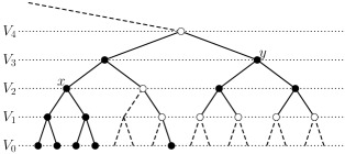
Two important graphs in this paper are paths and complete binary trees. PkP_{k} denotes the path graph of length kk (with k+1k+1 vertices and kk edges). TkT_{k} denotes the complete binary tree of height kk (with 2k+112^{k+1}-1 vertices and 2k+122^{k+1}-2 edges). We also consider infinite versions of these graphs. PP_{\infty} is the path graph with vertex set \mathbb{Z} and edge set {(i,i+1):i}\{(i,i+1):i\in\mathbb{Z}\}. TT_{\infty} is the union k=1Tk\bigcup_{k=1}^{\infty}T_{k} under the nesting T1T2T3T_{1}\subset T_{2}\subset T_{3}\subset\cdots where Leaves(T1)Leaves(T2)Leaves(T3)\mathrm{Leaves}(T_{1})\subset\mathrm{Leaves}(T_{2})\subset\mathrm{Leaves}(T_{3})\subset\cdots. Thus, TT_{\infty} is an infinite, rootless, layered binary tree, with leaves in layer 0, their parents in level 11, etc.

We use terms graph invariant and graph parameter interchangeably in reference to real-valued functions on graphs that are invariant under isomorphism.

2.2 Threshold weightings

We describe a family of edge-weightings on graphs GG, which in the case of finite graphs correspond to product distributions that are balanced with respect to the problem SUB(G)\mathrm{SUB}(G). (Definitions in this section are adapted from [8].)

Definition 2.1.

For any graph GG and function θ:E(G)\theta:E(G)\to\mathbb{R}, we denote by Δθ:{\Delta_{\theta}:\{finite subgraphs of G}G\}\to\mathbb{R} the function

Δθ(F):=|V(F)|eE(F)θ(e).\displaystyle\Delta_{\theta}(F)\vcentcolon=|V(F)|-\sum_{e\in E(F)}\theta(e).
Definition 2.2.

A threshold weighting for a graph GG is a function θ:E(G)[0,2]\theta:E(G)\to[0,2] such that Δθ(F)0\Delta_{\theta}(F)\geq 0 for all finite subgraphs FGF\subseteq G; if GG is finite, we additionally require that Δθ(G)=0\Delta_{\theta}(G)=0.

We refer to the pair (G,θ)(G,\theta) as a threshold-weighted graph. When θ\theta is fixed, we will at times simply write Δ()\Delta(\cdot) instead of Δθ()\Delta_{\theta}(\cdot).

Definition 2.3.

A Markov chain on a graph GG is a matrix [0,1]V(G)×V(G)[0,1]^{V(G)\times V(G)} that satisfies

  • wV(G)Mv,w=1\sum_{w\in V(G)}M_{v,w}=1 for all vV(G)v\in V(G) and

  • Mv,w>0{v,w}E(G)M_{v,w}>0\,\Longrightarrow\,\{v,w\}\in E(G) for all v,wV(G)v,w\in V(G).

Lemma 2.4.

Every Markov chain MM on GG induces a threshold weighting θ\theta on GG defined by

θ({v,w}):=Mv,w+Mw,v.\displaystyle\theta(\{v,w\})\vcentcolon=M_{v,w}+M_{w,v}.

This threshold weighting satisfies

Δθ(F)=vV(F)wV(G):{v,w}E(F)Mv,w.\displaystyle\Delta_{\theta}(F)=\sum_{v\in V(F)}\,\sum_{w\in V(G)\,:\,\{v,w\}\notin E(F)}M_{v,w}.

We remark that this lemma has a converse (shown in [11]): Every threshold weighting on GG is induced by a (not necessarily unique) Markov chain on GG. Lemma 2.4 also gives us a way to define threshold weightings when GG is an infinite graph; this will be useful later on.

Example 2.5.

Let MM be the transition matrix of the uniform random walk on TkT_{k} where k2k\geq 2. That is,

Mv,w:={1/deg(v)if {v,w}E(Tk),0otherwise.\displaystyle M_{v,w}\vcentcolon=\begin{cases}1/\mathrm{deg}(v)&\text{if }\{v,w\}\in E(T_{k}),\\ 0&\text{otherwise.}\end{cases}

For the associated threshold weighting θ:E(Tk)[0,2]\theta:E(T_{k})\to[0,2], we have

θ(e)={4/3if e contains a leaf,5/6if e contains the root,2/3otherwise.\displaystyle\theta(e)=\begin{cases}4/3&\text{if $e$ contains a leaf},\\ 5/6&\text{if $e$ contains the root},\\ 2/3&\text{otherwise.}\end{cases}

A key property of this θ\theta that we will use later on (Lemma 3.8) is that

Δθ(F)|V(F)V(TkF)|3\displaystyle\Delta_{\theta}(F)\geq\frac{|V(F)\cap V(T_{k}\setminus F)|}{3}

(that is, Δθ(F)\Delta_{\theta}(F) is at least one-third the size of the boundary of FF) for all graphs FTkF\subseteq T_{k}. This is a straightforward consequence of Lemma 2.4, which is also true in the infinite tree TT_{\infty}.

Example 2.6.

Let PkP_{k} be the path of length kk (with k+1k+1 vertices and kk edges). The constant function θ1+1k\theta\equiv 1+\frac{1}{k} is a threshold weighting for PkP_{k}. (This is different from the threshold function induced by the uniform random walk on PkP_{k}, which has value 1/21/2 on the two outer edges of PkP_{k} and value 11 on the inner edges.)

This example again makes sense for k=k=\infty. The constant function E(P){1}E(P_{\infty})\mapsto\{1\} is a threshold weighting for PP_{\infty}. This threshold function has the nice property that

Δ(F)=|V(F)||E(F)|=#{connected components of F}\displaystyle\Delta(F)=|V(F)|-|E(F)|=\#\{\text{connected components of }F\}

for all finite subgraphs FPF\subset P_{\infty}.

Definition 2.7.

Let GG be a finite graph, let θ\theta be a threshold weigting on GG, and let nn be a positive integer. We denote by 𝑿θ,n\bm{X}_{\theta,n} be the random V(G)V(G)-colored graph (i.e., input distribution to SUB(G)\mathrm{SUB}(G)) with vertex set V(G)×[n]V(G)\times[n], vertex-coloring (v,i)v(v,i)\mapsto v, and random edge relation given by

[{(v,i),(w,j)} is an edge of 𝑿θ,n]={1/nθ({v,w})if {v,w}E(G),0otherwise,\displaystyle\operatorname*{\mathds{P}}[\,\{(v,i),(w,j)\}\text{ is an edge of }\bm{X}_{\theta,n}\,]=\begin{cases}1/n^{\theta(\{v,w\})}&\text{if }\{v,w\}\in E(G),\\ 0&\text{otherwise,}\end{cases}

independently for all {(v,i),(w,j)}(V(G)×[n]2)\{(v,i),(w,j)\}\in\binom{V(G)\times[n]}{2}.

Lemma 2.8 ([8]).

The probability that 𝐗θ,n\bm{X}_{\theta,n} is a YES-instance of SUB(G)\mathrm{SUB}(G) is bounded away from 0 and 11.

The lower bounds of Theorem 1.2 and 1.3 are in fact average-case lower bounds for SUB(G)\mathrm{SUB}(G) under 𝑿θ,n\bm{X}_{\theta,n} for arbitrary threshold weightings θ\theta. Parameters κ(G)\kappa(G) and τ(G)\tau(G) are obtained by taking the optimal choice of threshold weighting θ\theta, as we describe in the next subsection.

2.3 Join-trees and parameters κ(G)\kappa(G) and τ(G)\tau(G)

Parameters κ(G)\kappa(G) and τ(G)\tau(G) are defined in terms of a notion called join-trees for subgraphs of GG. A join-tree is simply a “formula” computing a subgraph of GG, starting from individual edges, where union (\cup) is the only operation.

Definition 2.9.

A join-tree over GG is a finite rooted binary tree AA together with a labeling labelA:Leaves(A)E(G){}\mathrm{label}_{A}:\mathrm{Leaves}(A)\to E(G)\cup\{\bot\} (which may also be viewed as a partial function LeavesE(G)\mathrm{Leaves}\rightharpoonup E(G)). We reserve symbols A,B,C,D,EA,B,C,D,E for join-trees. (FF will always denote a subgraph of GG.)

The graph of AA, denoted GAG_{A}, is the subgraph of GG with edge set E(G)Range(labelA)E(G)\cap\mathrm{Range}(\mathrm{label}_{A}). (Note that GAG_{A} is always finite.) As a matter of notation, we write E(A)E(A) for E(GA)E(G_{A}) and V(A)V(A) for V(GA)V(G_{A}). We also write Δθ(A)\Delta_{\theta}(A) for Δθ(GA)\Delta_{\theta}(G_{A}) where θ\theta is a threshold weighting on GG.

We write \langle\rangle for the single-node join-tree labeled by \bot. For eE(G)e\in E(G), we write e\langle e\rangle for the single-node join-tree labeled by ee. For join-trees BB and CC, we write B,C\langle B,C\rangle for the join-tree consisting a root with BB and CC as children (with the inherited labels, i.e., labelB,C=labelBlabelC\mathrm{label}_{\langle B,C\rangle}=\mathrm{label}_{B}\cup\mathrm{label}_{C}). Note that GB,C=GBGCG_{\langle B,C\rangle}=G_{B}\cup G_{C}.

Every join-tree AA is clearly either \langle\rangle, or e\langle e\rangle where eE(G)e\in E(G), or B,C\langle B,C\rangle where B,CB,C are join-trees. In the first two cases, we say that AA is atomic; in the third case, we say that AA is non-atomic.

We say that BB is a child of AA if A{B,C,C,B}A\in\{\langle B,C\rangle,\langle C,B\rangle\} for some CC. We say that DD is a sub-join-tree of AA (denoted DAD\preceq A) if D=D=\langle\rangle or D=AD=A or DD is a sub-join-tree of a child of AA. We say that DD is a proper sub-join-tree (denoted DAD\prec A) if DAD\preceq A and DAD\neq A.

We are now able to define the invariant κ(G)\kappa(G) in Theorem 1.2, which lower bounds the restricted circuit size of SUB(G)\mathrm{SUB}(G). (In fact, κ(G)\kappa(G) also provides a nearly tight upper bound on the average-case AC0\textsl{AC}^{\,\textsl{0}} circuit size of SUB(G)\mathrm{SUB}(G) [11].)

Definition 2.10 (The invariant κ(G)\kappa(G) of Theorem 1.2).

For finite graphs GG, let

κ(G):=maxthreshold weightings θ for Gminjoin-trees A with graph GmaxBAΔθ(B).\displaystyle\kappa(G)\vcentcolon=\max_{\text{threshold weightings $\theta$ for $G$}}\ \min_{\text{join-trees $A$ with graph $G$}}\ \max_{B\preceq A}\ \Delta_{\theta}(B).

The invariant of τ(G)\tau(G) of Theorem 1.3 is significantly more complicated to define. We postpone the definition to Section 5 and, in the meantime, focus on a simpler “potential function” on join-trees, denoted Φθ(A)\Phi_{\theta}(A), which we use to lower bound τ(G)\tau(G). In order to state the definition of Φθ(A)\Phi_{\theta}(A), we require the following operation \ominus (“restriction away from”) on graphs and join-trees.

Definition 2.11 (The operation \ominus on graphs and join-trees).

For FGF\subseteq G and a subset SV(G)S\subseteq V(G), we denote by FSF\ominus S the graph consisting of the connected components of FF that are vertex-disjoint from SS.

For a join-tree AA, we denote ASA\ominus S the join-tree with the same rooted tree structure as AA and leaf labeling function

labelAS(l)\displaystyle\mathrm{label}_{A\ominus S}(l) :={labelA(l)if labelA(l)E(GAS),otherwise.\displaystyle\vcentcolon=\begin{cases}\mathrm{label}_{A}(l)&\text{if }\mathrm{label}_{A}(l)\in E(G_{A}\ominus S),\\ \bot&\text{otherwise.}\end{cases}

That is, ASA\ominus S deletes all labels except for edges in GASG_{A}\ominus S. Note that GAS=GASG_{A\ominus S}=G_{A}\ominus S.

As a matter of notation, if BB is another join-tree, we write ABA\ominus B for AV(B)A\ominus V(B) and A(SB)A\ominus(S\cup B) for A(SV(B))A\ominus(S\cup V(B)).

Refer to caption
Figure 1: An example where AA is a join-tree whose graph GAG_{A} consists of two paths of length 22 with edges e,f,g,he,f,g,h. SS is the set containing just the external endpoint of hh. The join-tree ASA\ominus S is depicted to the right.
Definition 2.12 (The potential function Φθ\Phi_{\theta} on join-trees).

Fix a threshold weighting θ\theta on a graph GG. The potential function Φθ:{\Phi_{\theta}:\{join-trees over G}0G\}\to\mathbb{R}_{\geq 0} is the unique pointwise minimum function satisfying the following inequalities for all join-trees A,B,C,DA,B,C,D:

({\dagger}) Φθ(A)\displaystyle\Phi_{\theta}(A) Φθ(D)+Δθ(CD)+Δθ(A(CD))\displaystyle\geq\Phi_{\theta}(D)+\Delta_{\theta}(C\ominus D)+\Delta_{\theta}(A\ominus(C\cup D)) if A{B,C,C,B} and DB,\displaystyle\text{if $A\in\{\langle B,C\rangle,\langle C,B\rangle\}$ and $D\preceq B$},
({\ddagger}) Φθ(A)\displaystyle\Phi_{\theta}(A) 12(Φθ(D)+Φθ(ED)+Δθ(A)+Δθ(A(DE)))\displaystyle\geq\frac{1}{2}\Big{(}\Phi_{\theta}(D)+\Phi_{\theta}(E\ominus D)+\Delta_{\theta}(A)+\Delta_{\theta}(A\ominus(D\cup E))\Big{)} if D,EA.\displaystyle\text{if $D,E\prec A$}.

Alternatively, Φθ(A)\Phi_{\theta}(A) has the following recursive characterization:

  • If AA is an atomic join-tree, then

    Φθ(A):=Δθ(A)={0if A=,2θ(e)if A=e where eE(G).\displaystyle\Phi_{\theta}(A)\vcentcolon=\Delta_{\theta}(A)=\begin{cases}0&\text{if }A=\langle\rangle,\\ 2-\theta(e)&\text{if $A=\langle e\rangle$ where $e\in E(G)$}.\end{cases}

    (Obs: In the case A=eA=\langle e\rangle, the constraint Φθ(A)Δθ(A)\Phi_{\theta}(A)\geq\Delta_{\theta}(A) is forced by ({\ddagger}) where B=C=B=C=\langle\rangle.)

  • If A=B,CA=\langle B,C\rangle, then

    Φθ(A):=max{maxDBΦθ(D)+Δθ(CD)+Δθ(A(CD)),maxDCΦθ(D)+Δθ(BD)+Δθ(A(BD)),maxD,EA12(Φθ(D)+Φθ(ED)+Δθ(A)+Δθ(A(DE)))}.\displaystyle\Phi_{\theta}(A)\vcentcolon=\max\left\{\begin{aligned} &\max_{\ D\preceq B\ }\ \Phi_{\theta}(D)+\Delta_{\theta}(C\ominus D)+\Delta_{\theta}(A\ominus(C\cup D)),\\ &\max_{\ D\preceq C\ }\ \Phi_{\theta}(D)+\Delta_{\theta}(B\ominus D)+\Delta_{\theta}(A\ominus(B\cup D)),\\ &\max_{D,E\prec A}\,\smash{\frac{1}{2}}\Big{(}\Phi_{\theta}(D)+\Phi_{\theta}(E\ominus D)+\Delta_{\theta}(A)+\Delta_{\theta}(A\ominus(D\cup E))\Big{)}\end{aligned}\right\}.

That is, at least one of inequalities ({\dagger}) or ({\ddagger}) is tight for each join-tree AA.

This definition, although opaque at first, will be clarified later (in Sections 4 and 5). The key property of Φθ(A)\Phi_{\theta}(A) is that it provides a lower bound the invariant τ(G)\tau(G), which in turn provides a lower bound on the restricted formula complexity of SUB(G)\mathrm{SUB}(G).

Theorem 2.13 ([16]).

The invariant τ(G)\tau(G) of Theorem 1.3 satisfies

τ(G)maxthreshold weightings θ for Gminjoin-trees A with graph GΦθ(A).\displaystyle\tau(G)\geq\max_{\textup{threshold weightings $\theta$ for $G$}}\ \min_{\textup{join-trees $A$ with graph $G$}}\ \Phi_{\theta}(A).

The definition of τ(G)\tau(G) and proof of Theorem 2.13 are postponed to Section 5. First, in Section 3, we will present our combinatorial main lemma, which gives a lower bound on Φθ(A)\Phi_{\theta}(A) for all join-trees with graph TkT_{k} under the threshold weighting θ\theta of Example 2.5.

2.4 Observations about Φθ\Phi_{\theta}

Note that inequality ({\dagger}) implies Φθ(A)Φθ(D)\Phi_{\theta}(A)\geq\Phi_{\theta}(D) for all DAD\preceq A (since Δθ()\Delta_{\theta}(\cdot) is nonnegative). Also note that inequality ({\ddagger}) implies Φθ(A)Δθ(A)\Phi_{\theta}(A)\geq\Delta_{\theta}(A) in the special case B=C=B=C=\langle\rangle (since Φθ()=0\Phi_{\theta}(\langle\rangle)=0 and A(A\ominus(the empty graph)=A)=A). Combining these observations, we see that Φθ(A)Δθ(D)\Phi_{\theta}(A)\geq\Delta_{\theta}(D) for all DAD\preceq A. It follows that τ(G)κ(G)\tau(G)\geq\kappa(G) for all graphs GG, which makes sense in light of the fact that κ(G)\kappa(G) bounds circuit size and τ(G)\tau(G) bounds formula size.

Next, observe that Φθ(A)\Phi_{\theta}(A) always equals either Φθ(D)+(some Δθ()-terms)\Phi_{\theta}(D)+(\text{some $\Delta_{\theta}(\cdot)$-terms}) or 12(Φθ(D)+Φθ(ED))+(some Δθ()-terms)\frac{1}{2}(\Phi_{\theta}(D)+\Phi_{\theta}(E\ominus D))+(\textit{some $\Delta_{\theta}(\cdot)$-terms}) where DD and EE are proper sub-join-trees of AA. This can be expanded out until we get a nonnegative linear combination of Δθ()\Delta_{\theta}(\cdot)-terms. Looking closely, we see that

Φθ(A)=FGcFΔθ(F)\displaystyle\Phi_{\theta}(A)=\sum_{F\subseteq G}c_{F}\cdot\Delta_{\theta}(F)

where coefficients cFc_{F} (which depend on both θ\theta and AA) are nonnegative dyadic rational numbers coming from the tight instances of inequalities ({\dagger}) and ({\ddagger}). We may further observe, for any vV(G)v\in V(G), that

FG:vV(F)cF1.\displaystyle\sum_{F\subseteq G\,:\,v\in V(F)}c_{F}\leq 1.

This is easily shown by induction using the fact that graphs F1F_{1} and F2F1F_{2}\ominus F_{1} and F3(F1F2)F_{3}\ominus(F_{1}\cup F_{2}) are pairwise disjoint for any F1,F2,F3GF_{1},F_{2},F_{3}\subseteq G.

One consequence of this observation is the following lemma, which we will use in Sections 3 and 6.

Lemma 2.14.

Suppose (G,θ)(G,\theta) and (G,θ)(G^{\ast},\theta^{\ast}) are threshold-weighted graphs such that GGG\subseteq G^{\ast} and θ(e)θ(e)\theta^{\ast}(e)\leq\theta(e) for all eE(G)e\in E(G). Then for any join-tree AA with graph GG, we have

Φθ(A)Φθ(A)eE(G)(θ(e)θ(e)).\displaystyle\Phi_{\theta}(A)\geq\Phi_{\theta^{\ast}}(A)-\sum_{e\in E(G)}\Big{(}\theta(e)-\theta^{\ast}(e)\Big{)}.
Proof.

Let {cF}FG\{c_{F}\}_{F\subseteq G} be nonnegative dyadic rationals — arising from the tight instances of inequalities ({\dagger}) and ({\ddagger}) in the recursive definition of Φθ(A)\Phi_{\theta^{\ast}}(A) — such that Φθ(A)=FGcFΔθ(F)\Phi_{\theta^{\ast}}(A)=\sum_{F\subseteq G}c_{F}\cdot\Delta_{\theta^{\ast}}(F). We may apply inequalities ({\dagger}) and ({\ddagger}) in the exact same way to get the bound Φθ(A)FGcFΔθ(F)\Phi_{\theta}(A)\geq\sum_{F\subseteq G}c_{F}\cdot\Delta_{\theta}(F). We now have

Φθ(A)Φθ(A)\displaystyle\Phi_{\theta^{\ast}}(A)-\Phi_{\theta}(A) FGcF(Δθ(F)Δθ(F))\displaystyle\leq\sum_{F\subseteq G}c_{F}\Big{(}\Delta_{\theta^{\ast}}(F)-\Delta_{\theta}(F)\Big{)}
=FGcFeE(F)(θ(e)θ(e))\displaystyle=\sum_{F\subseteq G}c_{F}\sum_{e\in E(F)}\Big{(}\theta(e)-\theta^{\ast}(e)\Big{)}
=eE(G)(θ(e)θ(e))FG:eE(F)cF\displaystyle=\sum_{e\in E(G)}\Big{(}\theta(e)-\theta^{\ast}(e)\Big{)}\sum_{F\subseteq G\,:\,e\in E(F)}c_{F}
eE(G)(θ(e)θ(e)),\displaystyle\leq\sum_{e\in E(G)}\Big{(}\theta(e)-\theta^{\ast}(e)\Big{)},

using the fact that θ(e)θ(e)0\theta(e)-\theta^{\ast}(e)\geq 0 and FG:vV(F)cF1\sum_{F\subseteq G\,:\,v\in V(F)}c_{F}\leq 1 for all vV(G)v\in V(G). ∎

2.5 Lower bounds on Φθ\Phi_{\theta}

Having introduced the potential function Φθ\Phi_{\theta} and described its connection to τ\tau in Theorem 2.13, we conclude this section by briefly explaining how it is used derive lower bounds τ(Pk)\tau(P_{k}) and τ(Tk)\tau(T_{k}). The main combinatorial lemma behind the lower bound of Theorem 1.9 is the following:

Lemma 2.15 ([15]).

Let θ\theta be the constant 1+1k1+\frac{1}{k} threshold weighting on PkP_{k}. For every join-tree AA with graph PkP_{k}, we have Φθ(A)12log13+1(k)\Phi_{\theta}(A)\geq\frac{1}{2}\log_{\sqrt{13}+1}(k). (Therefore, τ(G)12log13+1(k)\tau(G)\geq\frac{1}{2}\log_{\sqrt{13}+1}(k).)

The proof is included in Appendix A, for the sake of comparison with our two lower bounds below. We remark that this proof makes crucial use of both ({\dagger}) and ({\ddagger}); it was shown in [15] that no lower bound better than Φθ(A)=Ω(1)\Phi_{\theta}(A)=\Omega(1) is provable using ({\dagger}) alone or ({\ddagger}) alone.

Our lower bound τ(Tk)=Ω(k)\tau(T_{k})=\Omega(k) (Theorem 1.7) is an immediate consequence of the following:

Lemma 2.16.

Let θ\theta be the threshold weighting arising from the uniform random walk on TkT_{k} (Example 2.5). For every join-tree AA with graph TkT_{k}, we have Φθ(A)k/301/5\Phi_{\theta}(A)\geq k/30-1/5.

Our proof, given in the next section, is purely graph-theoretic. Interestingly, the argument essentially uses only inequality ({\ddagger}); we do not require ({\dagger}), other than in the weak form Φθ(A)Φθ(D)\Phi_{\theta}(A)\geq\Phi_{\theta}(D) for all DAD\prec A.

It is worth mentioning that the choice of threshold weighting is important in Lemma 2.16. A different, perhaps more obvious, threshold weighting is the constant function with value |V(Tk)||E(Tk)|\frac{|V(T_{k})|}{|E(T_{k})|} (=2k+112k+12=\frac{2^{k+1}-1}{2^{k+1}-2}). With respect to this threshold weighting, no lower bound better than Ω(1)\Omega(1) is possible.

Finally, our improved lower bound τ(Pk)log5+5(k)\tau(P_{k})\geq\log_{\sqrt{5}+5}(k) (Theorem 1.11) is obtained via the following lemma. This result involves a 2-parameter extension of Φθ(A)\Phi_{\theta}(A) denoted Φθ(A|S)\Phi_{\theta}(A|S) (where SV(G)S\subseteq V(G)), which we introduce in Section 4.

Lemma 2.17.

Let θ\theta be the constant 1+1k1+\frac{1}{k} threshold weighting on PkP_{k}. For every join-tree AA with graph PkP_{k}, we have Φθ(A|)log5+5(k)1\Phi_{\theta}(A|\emptyset)\geq\log_{\sqrt{5}+5}(k)-1.

This lemma is proved in Section 6, after we show how Φθ(|)\Phi_{\theta}(\cdot|\cdot) provides a lower bound on τ()\tau(\cdot) in Section 5.

3 Lower bound τ(Tk)=Ω(k)\tau(T_{k})=\Omega(k)

We fix the infinite pattern graph TT_{\infty} with the threshold weighting θ\theta induced by the uniform random walk. Recall that T=k=1TkT_{\infty}=\bigcup_{k=1}^{\infty}T_{k} under a nesting T1T2T3T_{1}\subset T_{2}\subset T_{3}\subset\cdots with Leaves(T1)Leaves(T2)Leaves(T3)\mathrm{Leaves}(T_{1})\subset\mathrm{Leaves}(T_{2})\subset\mathrm{Leaves}(T_{3})\subset\cdots. F,G,HF,G,H will represent finite subgraphs of TT_{\infty}, and A,B,C,D,EA,B,C,D,E will be join-trees over TT_{\infty}. (In particular, note that GG no longer denotes the ambient pattern graph.)

We next recall the definition of θ\theta from Example 2.5. Let M[0,1]V(T)×V(T)M\in[0,1]^{V(T_{\infty})\times V(T_{\infty})} be the transition matrix of the uniform random walk on TT_{\infty}, that is,

Mv,w={1if {v,w}E(T) and v is a leaf,1/3if {v,w}E(T) and v is a non-leaf,0if {v,w}E(T).\displaystyle M_{v,w}=\begin{cases}1&\text{if $\{v,w\}\in E(T_{\infty})$ and $v$ is a leaf,}\\ 1/3&\text{if $\{v,w\}\in E(T_{\infty})$ and $v$ is a non-leaf,}\\ 0&\text{if $\{v,w\}\notin E(T_{\infty})$.}\end{cases}

This induces the threshold weighting θ:E(T)[0,2]\theta:E(T_{\infty})\to[0,2] given by

θ({v,w}):=Mv,w+Mw,v={2/3if v or w is a leaf of T,4/3otherwise.\displaystyle\theta(\{v,w\})\vcentcolon=M_{v,w}+M_{w,v}=\begin{cases}2/3&\text{if $v$ or $w$ is a leaf of $T_{\infty}$},\\ 4/3&\text{otherwise.}\end{cases}

Since θ\theta is fixed, we will suppress it when writing Δ(F)\Delta(F) and Φ(A)\Phi(A).

Definition 3.1.

For all k0k\geq 0, let

Vk:={vV(Tk):v has distance k from a leaf}.\displaystyle V_{k}\vcentcolon=\{v\in V(T_{k}):v\text{ has distance $k$ from a leaf}\}.

Thus, V0V_{0} is the set of leaves in TT_{\infty}, V1V_{1} is the set of parents of leaves, etc. Note that V(T)=k=0VkV(T_{\infty})=\bigcup_{k=0}^{\infty}V_{k}. We shall refer to the VkV_{k} as the various levels of TT_{\infty}.

For k1k\geq 1 and xVkx\in V_{k}, let TxTT_{x}\subset T_{\infty} be the complete binary tree of height kk rooted at xx (in the case k=0k=0, we regard TxT_{x} as a single isolated vertex). We denote by Tx+T_{x}^{+} the graph obtained from TxT_{x} by including an extra edge between xx and its parent. Note that

|V(Tx)|=2k+11,|V(Tx+)|=2k+1,|E(Tx)|=2k+12,|V(Tx+)|=2k+11.\displaystyle|V(T_{x})|=2^{k+1}-1,\qquad|V(T_{x}^{+})|=2^{k+1},\qquad|E(T_{x})|=2^{k+1}-2,\qquad|V(T_{x}^{+})|=2^{k+1}-1.

For j{0,,k}j\in\{0,\dots,k\}, let Vj(Tx):=VjV(Tx)V_{j}(T_{x})\vcentcolon=V_{j}\cap V(T_{x}).

Observation 3.2.

If xVkx\in V_{k}, then for j{0,,k}j\in\{0,\dots,k\}, |Vj(Tx)|=2kj|V_{j}(T_{x})|=2^{k-j}.

We next define two useful parameters of finite subgraphs of TT_{\infty}.

Definition 3.3 (Max-complete height).

For a finite subgraph FF of TT_{\infty}, define the max-complete height λ(F)\lambda(F) to be the maximum kk\in\mathbb{N} for which there exists xVkx\in V_{k} with TxGT_{x}\subseteq G; λ(F)\lambda(F) is defined to be zero when no such xx exists (in particular, this happens when V(F)V0=V(F)\cap V_{0}=\emptyset).

Observation 3.4.

For any xVkx\in V_{k}, λ(Tx)=λ(Tx+)=k\lambda(T_{x})=\lambda(T_{x}^{+})=k.

Definition 3.5 (Boundary size).

Let (F)\partial(F) denote the size of boundary of FF in TT_{\infty}:

(F):=|V(F)V(TF)|.\displaystyle\partial(F)\vcentcolon=|V(F)\cap V(T_{\infty}\setminus F)|.
Observation 3.6.

For any xVkx\in V_{k}, we have (Tx)=(Tx+)=1\partial(T_{x})=\partial(T_{x}^{+})=1, as the boundaries in the respective graphs are simply the singletons {x}\{x\} and {parent(x)}\{\mathrm{parent}(x)\}. Another example is as follows: if xVkx\in V_{k} for some k2k\geq 2 and FF is the subgraph of TxT_{x} induced by the set of vertices V(Tx)V0V(T_{x})\setminus V_{0}, then (F)=2k1+1\partial(F)=2^{k-1}+1 as all vertices in V1(Tx)V_{1}(T_{x}) (along with xx) lie in the boundary of FF.

Definition 3.7 (Grounded and ungrounded subgraphs of TT_{\infty}).

Let F,HF,H be finite subgraphs of TT_{\infty}. We say that FF is grounded if it is connected and V(F)V0V(F)\cap V_{0}\neq\emptyset (that is, FF is a tree, at least one of whose leaves is also a leaf of TT_{\infty}). We say that HH is ungrounded if it is non-empty and connected and V(H)V0=V(H)\cap V_{0}=\emptyset (that is, HH is a non-empty tree, none of whose leaves is a leaf of TT_{\infty}).

Refer to caption
Figure 2: Example of a grounded graph FTF\subset T_{\infty}. The dotted lines indicate the various levels that V(F)V(F) intersects and dashed lines indicate (some of the) edges in TFT_{\infty}\setminus F. The nodes colored white lie in the boundary of FF, and therefore (F)=7\partial(F)=7 and Δ(F)=11/3\Delta(F)=11/3. The max-complete height λ(F)=2\lambda(F)=2, since TxFT_{x}\subset F for xV2x\in V_{2} and xx is the highest such node. The subgraph H=FTyH=F\cap T_{y} is ungrounded with λ(H)=0\lambda(H)=0.

We shall think of the function (F)\partial(F) as essentially a proxy for Δ(F)\Delta(F), as it has the advantage of having a simple combinatorial definition. This is justified by the following:

Lemma 3.8.

For every FTF\subset T_{\infty}, we have Δ(F)(F)/3\Delta(F)\geq\partial(F)/3.

It also holds that Δ(F)2(F)/3\Delta(F)\leq 2\partial(F)/3 for FF without isolated vertices (or Δ(F)(F)\Delta(F)\leq\partial(F) if we allow isolated vertices), but we will not need this upper bound.

Proof.

Since θ\theta is the threshold weighting induced by MM, Lemma 2.4 tells us

Δ(F)=vV(F)wV(T):{v,w}E(TF)Mv,w.\displaystyle\Delta(F)=\sum_{v\in V(F)}\ \sum_{w\in V(T_{\infty})\,:\,\{v,w\}\in E(T_{\infty}\setminus F)}M_{v,w}.

Note that vV(F)v\in V(F) contributes to this sum if, and only if, it belongs to the boundary of FF (i.e., vV(F)V(TF)v\in V(F)\cap V(T_{\infty}\setminus F)). Since Mv,w1/3M_{v,w}\geq 1/3 whenever {v,w}E(F)\{v,w\}\in E(F), the claim follows. ∎

We are now ready to state the main theorem of the section.

Theorem 3.9.

Let ε=1/30\varepsilon=1/30 and δ=2/5\delta=2/5. Then for every join-tree AA,

Φ(A)ελ(A)+δΔ(A).\displaystyle\Phi(A)\geq\varepsilon\lambda(A)+\delta\Delta(A).

Theorem 3.9 directly implies Lemma 2.16, which in turn yields the lower bound τ(Tk)=Ω(k)\tau(T_{k})=\Omega(k) of Theorem 1.7. To see why, let θ\theta^{\prime} be the threshold weighting on TkT_{k} coming from the uniform random walk (Example 2.5). Viewing TkT_{k} a subgraph of TT_{\infty}, note that eE(Tk)(θ(e)θ(e))=2(5623)=13\sum_{e\in E(T_{k})}(\theta^{\prime}(e)-\theta(e))=2(\frac{5}{6}-\frac{2}{3})=\frac{1}{3}. For any join-tree AA with graph TkT_{k}, Lemma 2.14 and Theorem 3.9 now imply

Φθ(A)Φ(A)13130λ(Tk)+25Δ(Tk)13=130k+251313=130k15.\displaystyle\Phi_{\theta^{\prime}}(A)\geq\Phi(A)-\frac{1}{3}\geq\frac{1}{30}\lambda(T_{k})+\frac{2}{5}\Delta(T_{k})-\frac{1}{3}=\frac{1}{30}k+\frac{2}{5}\cdot\frac{1}{3}-\frac{1}{3}=\frac{1}{30}k-\frac{1}{5}.

We proceed with a few definitions and lemmas needed for the proof of Theorem 3.9 in Section 3.1. In order to present the main arguments first, proofs of three auxiliary lemmas (3.10, 3.12, 3.13) are postponed to Section 3.2.

Lemma 3.10.

Let HH be a non-empty finite subgraph of TT_{\infty}, all of whose components are ungrounded. Then (H)12(|E(H)|+3)\partial(H)\geq\frac{1}{2}(|E(H)|+3).

We make a note of its following corollary here.

Corollary 3.11.

Suppose HH be a finite connected subgraph of TT_{\infty} and yV(H)y\in V(H) such that E(H)E(Ty)E(H)\cap E(T_{y})\neq\emptyset and HH does not contain any path from yy to a leaf of TyT_{y}. Then (H)12(|E(H)E(Ty)|+1)\partial(H)\geq\frac{1}{2}(|E(H)\cap E(T_{y})|+1).

Proof.

Let FF be the graph with edge set E(F)E(H)E(Ty)E(F)\coloneqq E(H)\cap E(T_{y}). Note that FF is non-empty, connected and ungrounded. Observe that (H)(F)1\partial(H)\geq\partial(F)-1 because all vertices in the boundary of HH, with the only possible exception of yy, also lie in the boundary of FF. Hence by Lemma 3.10, (H)12(|E(H)E(Ty)|+1)\partial(H)\geq\frac{1}{2}(|E(H)\cap E(T_{y})|+1). ∎

The second auxiliary lemma gives a useful inequality relating (G)\partial(G), λ(G)\lambda(G) and |E(G)||E(G)|.

Lemma 3.12.

For every finite subgraph GG of TT_{\infty}, we have λ(G)+(G)log(|E(G)|+1)\lambda(G)+\partial(G)\geq\log(|E(G)|+1).

(This is tight when G=Tx+G=T_{x}^{+} for some xVkx\in V_{k}, in which case λ(G)=k\lambda(G)=k and (G)=1\partial(G)=1 and |E(G)|=2k+11|E(G)|=2^{k+1}-1.) The third auxiliary lemma shows that subgraphs of TkT_{k} that contain at most half the edges of TkT_{k} and have boundary size jj (k/2\leq k/2) have empty intersection with a large complete subtree of TkT_{k} of height kjk-j.

Lemma 3.13.

Let xVkx\in V_{k} and suppose GTxG\subseteq T_{x} such that |E(GTx)|2k1|E(G\cap T_{x})|\leq 2^{k}-1 and (G)k/6\partial(G)\leq k/6. Then there exists a vertex zVk(G)(Tx)z\in V_{k-\partial(G)}(T_{x}) such that E(G)E(Tz+)=E(G)\cap E(T^{+}_{z})=\emptyset.

We now state and prove the main lemma used in the proof of Theorem 3.9.

Lemma 3.14.

For any integers 1t1\leq t\leq\ell, let zVz\in V_{\ell} and suppose AA is a join-tree such that TzGAT_{z}\subseteq G_{A}. Then one the following conditions holds:

  1.  (i)

    There exists DAD\preceq A such that (D)t\partial(D)\geq t and λ(D)+(D)\lambda(D)+\partial(D)\geq\ell.

  2.  (ii)

    There exists CAC\prec A with λ((CTz){z})+((CTz){z})t\lambda((C\cap T_{z})\ominus\{z\})+\partial((C\cap T_{z})\ominus\{z\})\geq\ell-t.

  3.  (iii)

    There exists EAE\prec A such that (E)t\partial(E)\geq\ell-t.

Proof.

Descend in the join-tree AA until reaching a BAB\preceq A such that BB contains a path PP from zz to a leaf of TzT_{z}, but no BBB^{\prime}\prec B contains a path from zz to a leaf of TzT_{z}.

Let j{1,,}j\in\{1,\dots,\ell\} be maximal such that there exists yVj(Tz)Py\in V_{j}(T_{z})\cap P such that TyGBT_{y}\subseteq G_{B}. We claim that (B)j\partial(B)\geq\ell-j. To see this, note that for every vertex vyv\neq y on the path from zz to yy (a subpath of PP), if c(v)c(v) denotes the child of vv that is not on the path PP, then GG does not contain Tc(v)+T^{+}_{c(v)} (because if it did then λ(G)>k\lambda(G)>k). As a result, it must be the case that for every vertex vyv\neq y on the path from zz to yy, some vertex in V(GB)V(Tc(v)+)V(G_{B})\cap V(T^{+}_{c(v)}) lies in the boundary of GG and so, (G)j\partial(G)\geq\ell-j.

As an illustration of this argument, consider the graph GBG_{B} in Figure 3(a). Then for every vertex v{v2,,v5}v\in\{v_{2},\ldots,v_{5}\}, either vv itself is in the boundary (like v2v_{2} and v5v_{5}) or some vertex in Tc(v)T_{c(v)} is in the boundary (for v3v_{3}, it is c(v3)c(v_{3}) for example and for v4v_{4}, it is either child of c(v4)c(v_{4})).

Refer to caption
(a) Here j=1j=1 is “small”. For each i{2,,5}i\in\{2,\dots,5\}, either viv_{i} or a node in its right subtree lies in the boundary of BB.
Refer to caption
(b) CC doesn’t contain the path between yy and zz. So we can directly use Lemma 3.12 on (CTz){z}(C\cap T_{z})\ominus\{z\}.
Refer to caption
(c) CC contains the path from zz to yy and HTyH\cap T_{y} is “large”. But also HH is ungrounded and thus has large boundary.
Refer to caption
(d) HTyH\cap T_{y} is “small”. But then again, (CTz){z}(C\cap T_{z})\ominus\{z\} is large and so Lemma 3.12 is applicable.
Figure 3: An illustration with =5\ell=5, t=3t=3. In each example, solid lines denote the edges of BB, thickly shaded lines denote the subgraph CC, and dashed lines denote edges of TzBT_{z}\setminus B. Nodes shaded white lie in the boundary of BB (thought not necessarily the boundary of CC). PP is the path v0v1v2v3v4v5v_{0}v_{1}v_{2}v_{3}v_{4}v_{5}.

Consider the case that jtj\leq\ell-t (again see Figure 3(a)). Letting D:=BD\vcentcolon=B, we have (D)jt\partial(D)\geq\ell-j\geq t and λ(D)j\lambda(D)\geq j, so condition (i) is satisfied. We shall therefore proceed under the assumption that

jt+1.\displaystyle j\geq\ell-t+1.

Since TyGBT_{y}\subseteq G_{B}, at least one child CC of BB satisfies

|E(C)E(Ty)|12|E(Ty)|=2j1.\displaystyle|E(C)\cap E(T_{y})|\geq\frac{1}{2}|E(T_{y})|=2^{j}-1.

Fix one such CC.

Consider the case that CC does not contain the path between zz and yy (see Figure 3(b)). Then CTyC{z}C\cap T_{y}\subseteq C\ominus\{z\}, so by Lemma 3.12,

λ((CTz){z})+((CTz){z})\displaystyle\lambda((C\cap T_{z})\ominus\{z\})+\partial((C\cap T_{z})\ominus\{z\}) log(|E(CTy)|+1)log(2j)t+1.\displaystyle\geq\log(|E(C\cap T_{y})|+1)\geq\log(2^{j})\geq\ell-t+1.

In this case, we satisfy condition (ii). We shall therefore proceed under the assumption that CC contains the path between zz and yy.

Note that CC does not contain a path from yy to any leaf of TyT_{y} (since otherwise CC would contain a path from zz to a leaf of TzT_{z}, contradicting the way we choose BAB\preceq A). Let HH be the connected component of GCG_{C} that contains yy (and hence also contains the path between zz and yy).

We now consider two final cases, depending on the size of |E(H)E(Ty)||E(H)\cap E(T_{y})|. First, assume |E(H)E(Ty)|2(t)|E(H)\cap E(T_{y})|\geq 2(\ell-t) (see Figure 3(c)). In this case, Corollary 3.11 implies

(C)(H)12(|E(H)E(Ty)|+1)t.\displaystyle\partial(C)\geq\partial(H)\geq\frac{1}{2}\Big{(}|E(H)\cap E(T_{y})|+1\Big{)}\geq\ell-t.

We satisfy condition (iii) setting E:=CE\vcentcolon=C.

Finally, assume |E(H)E(Ty)|2(t)1|E(H)\cap E(T_{y})|\leq 2(\ell-t)-1 (see Figure 3(d)). We have

|E((CTz){z})|\displaystyle|E((C\cap T_{z})\ominus\{z\})| |E(C)E(Ty)||E(H)E(Ty)|\displaystyle\geq|E(C)\cap E(T_{y})|-|E(H)\cap E(T_{y})|
(2j1)(2(t)1)\displaystyle\geq(2^{j}-1)-(2(\ell-t)-1)
2t+12(t).\displaystyle\geq 2^{\ell-t+1}-2(\ell-t).

Lemma 3.12 now implies

λ((CTz){z})+((CTz){z})\displaystyle\lambda((C\cap T_{z})\ominus\{z\})+\partial((C\cap T_{z})\ominus\{z\}) log(|E((CTz){z})|+1)\displaystyle\geq\log(|E((C\cap T_{z})\ominus\{z\})|+1)
log(2t+12(t)+1)\displaystyle\geq\log(2^{\ell-t+1}-2(\ell-t)+1)
>t\displaystyle>\ell-t

since 2x+12x+1>2x2^{x+1}-2x+1>2^{x} for all x0x\geq 0. Therefore, condition (ii) is again satisfied in this final case. ∎

3.1 Proof of Theorem 3.9

We now prove Theorem 3.9: the lower bound Φ(A)ελ(A)+δΔ(A)\Phi(A)\geq\varepsilon\lambda(A)+\delta\Delta(A) where ε=1/30\varepsilon=1/30 and δ=2/5\delta=2/5.

We argue by a structural induction on join-trees AA. First, consider the case that GAG_{A} is empty, then Φ(A)=0\Phi(A)=0 and ελ(A)+δΔ(A)=0\varepsilon\lambda(A)+\delta\Delta(A)=0. We shall assume that GAG_{A} is non-empty.

Next consider the base case where AA is the atomic join-tree e\langle e\rangle for an edge eE(T)e\in E(T_{\infty}). In this case, we have λ(A)1\lambda(A)\leq 1 and

Φ(A)=Δ(A)={2/3if e contains a leaf,4/3otherwise.\displaystyle\Phi(A)=\Delta(A)=\begin{cases}2/3&\text{if $e$ contains a leaf,}\\ 4/3&\text{otherwise.}\end{cases}

Therefore, ελ(A)+δΔ(A)(1/30)+(2/5)(4/3)=17/30\varepsilon\lambda(A)+\delta\Delta(A)\leq(1/30)+(2/5)(4/3)=17/30. We are done, since Φ(A)2/3>ελ(A)+δΔ(A)\Phi(A)\geq 2/3>\varepsilon\lambda(A)+\delta\Delta(A).

From now on, let AA be a non-atomic join-tree with whose graph is non-empty. Let

k:=λ(A).\displaystyle k\vcentcolon=\lambda(A).

Our goal is thus to prove Φ(A)εk+δΔ(A)\Phi(A)\geq\varepsilon k+\delta\Delta(A), which we do by analyzing numerous cases.

Consider first the case that k=0k=0. In this case, we clearly have Φ(A)εk+δΔ(A)\Phi(A)\geq\varepsilon k+\delta\Delta(A) (since ΦΔ0\Phi\geq\Delta\geq 0 and δ<1\delta<1). So shall proceed on the assumption that k1k\geq 1.

Since ΦΔ\Phi\geq\Delta, we are done if Δ(A)εk+δΔ(A)\Delta(A)\geq\varepsilon k+\delta\Delta(A). So we shall proceed on the additional assumption that

(2) Δ(A)ε1δk=118k.\Delta(A)\leq\frac{\varepsilon}{1-\delta}k=\frac{1}{18}k.
Fixing xTkx\in T_{k} with TkGAT_{k}\subseteq G_{A}:

By definition of λ(A)\lambda(A), there exists a vertex xTkx\in T_{k} such that TkGAT_{k}\subseteq G_{A}. Let us fix any such xx.

Fixing BAB\preceq A with 2k1|E(B)E(Tx)|2k12^{k-1}\leq|E(B)\cap E(T_{x})|\leq 2^{k}-1:

We next fix a sub-join-tree BAB\preceq A satisfying 2k1|E(B)E(Tx)|2k12^{k-1}\leq|E(B)\cap E(T_{x})|\leq 2^{k}-1. To see that such BB exists, first note that |E(A)E(Tx)|=|E(Tx)|=2k+12|E(A)\cap E(T_{x})|=|E(T_{x})|=2^{k+1}-2. Consider a walk down AA which at each step descends to a child CC which maximizes |E(C)E(Tx)||E(C)\cap E(T_{x})|. This quantity shrinks by a factor 1/2\geq 1/2 at each step, eventually reaching size 11. Therefore, at some stage, we reach a sub-join-tree BB such that the intersection size |E(B)E(Tx)||E(B)\cap E(T_{x})| is between 2k12^{k-1} and 2k12^{k}-1.

Observe that Φ(A)Φ(B)Δ(B)\Phi(A)\geq\Phi(B)\geq\Delta(B) (by ({\dagger}) and the fact that ΦΔ\Phi\geq\Delta for all join-trees). Therefore, we are done if Δ(B)εk+δΔ(A)\Delta(B)\geq\varepsilon k+\delta\Delta(A). So we shall proceed under the additional assumption that

(3) Δ(B)εk+δΔ(A)=130k+25Δ(A)(130+25118)k=118k.\Delta(B)\leq\varepsilon k+\delta\Delta(A)=\frac{1}{30}k+\frac{2}{5}\Delta(A)\leq\Big{(}\frac{1}{30}+\frac{2}{5}\cdot\frac{1}{18}\Big{)}k=\frac{1}{18}k.

Since |E(B)||E(B)E(Tx)|2k1|E(B)|\geq|E(B)\cap E(T_{x})|\geq 2^{k-1}, Lemma 3.12 tells us that λ(B)+(B)k1\lambda(B)+\partial(B)\geq k-1. We make note of the fact that this implies

(4) Φ(B)\displaystyle\Phi(B) ελ(B)+δΔ(B)\displaystyle\geq\varepsilon\lambda(B)+\delta\Delta(B) (induction hypothesis)
ε(k(B)1)+δΔ(B)\displaystyle\geq\varepsilon\Big{(}k-\partial(B)-1\Big{)}+\delta\Delta(B)
εk+(δ3ε)Δ(B)ε\displaystyle\geq\varepsilon k+(\delta-3\varepsilon)\Delta(B)-\varepsilon (using 3Δ).\displaystyle\text{(using $-\partial\geq-3\Delta$)}.
Fixing zVk(B)(Tx)z\in V_{k-\partial(B)}(T_{x}) with E(B)E(Tz+)=E(B)\cap E(T_{z}^{+})=\emptyset:

Note that (B)3Δ(B)k/6\partial(B)\leq 3\Delta(B)\leq k/6 by (3). Since |E(B)E(Tx)|2k1|E(B)\cap E(T_{x})|\leq 2^{k}-1, the hypotheses of Lemma 3.13 are satisfied with respect to the vertex xx and the graph GBTxG_{B}\cap T_{x}. Therefore, we may fix a vertex zVk(B)(Tx)z\in V_{k-\partial(B)}(T_{x}) such that E(B)E(Tz+)=E(B)\cap E(T_{z}^{+})=\emptyset.

We next introduce a parameter

t:=6Δ(A)+3Δ(B).\displaystyle t\vcentcolon=6\Delta(A)+3\Delta(B).

Note that tt is an integer, since 3Δ3\Delta is integral. Our choice of parameters moreover ensure that 1tk/21\leq t\leq k/2, since Δ(A),Δ(B)k/18\Delta(A),\Delta(B)\leq k/18 by (2),(3) and Δ(A),Δ(B)1/3\Delta(A),\Delta(B)\geq 1/3 for all nonempty graphs. Since k(B)k3Δ(B)5k/6k-\partial(B)\geq k-3\Delta(B)\geq 5k/6, it follows that t<k(B)t<k-\partial(B).

Since zVk(B)z\in V_{k-\partial(B)} and TzTxGAT_{z}\subseteq T_{x}\subseteq G_{A}, Lemma 3.14 (with respect to zz and 1t<:=k(B)1\leq t<\ell\vcentcolon=k-\partial(B)) tells us that one of the following conditions holds:

  1.  (i)

    There exists DAD\preceq A such that (D)t\partial(D)\geq t and λ(D)+(D)k(B)\lambda(D)+\partial(D)\geq k-\partial(B).

  2.  (ii)

    There exists CAC\prec A with λ((CTz){z})+((CTz){z})k(B)t\lambda((C\cap T_{z})\ominus\{z\})+\partial((C\cap T_{z})\ominus\{z\})\geq k-\partial(B)-t.

  3.  (iii)

    There exists EAE\prec A with (E)k(B)t\partial(E)\geq k-\partial(B)-t.

We will show that Φ(A)εk+δΔ(A)\Phi(A)\geq\varepsilon k+\delta\Delta(A) in each of these three cases.

Case (i):

Suppose D=AD=A. Then it follows that (A)t>6Δ(A)\partial(A)\geq t>6\Delta(A), but this contradicts Lemma 3.8 by which Δ(A)(A)/3\Delta(A)\geq\partial(A)/3, as boundary of a non-empty graph is always non-empty. Thus, DAD\prec A and we have

Φ(A)()Φ(D)\displaystyle\Phi(A)\stackrel{{\scriptstyle({\dagger})}}{{\geq}}\Phi(D)\vphantom{\big{|}} ελ(D)+δΔ(D)\displaystyle\geq\varepsilon\lambda(D)+\delta\Delta(D) (induction hypothesis)
ελ(D)+δ3(D)\displaystyle\geq\varepsilon\lambda(D)+\frac{\delta}{3}\partial(D) (since Δ/3\Delta\geq\partial/3)
ε(k(B))+(δ3ε)(D)\displaystyle\geq\varepsilon\Big{(}k-\partial(B)\Big{)}+\Big{(}\frac{\delta}{3}-\varepsilon\Big{)}\partial(D) (since λ(D)+(D)k(B)\lambda(D)+\partial(D)\geq k-\partial(B) by Case (i))
ε(k(B))+(δ3ε)t\displaystyle\geq\varepsilon\Big{(}k-\partial(B)\Big{)}+\Big{(}\frac{\delta}{3}-\varepsilon\Big{)}t (since δ/3>ε\delta/3>\varepsilon and (D)t\partial(D)\geq t by Case (i))
=ε(k(B))+(δ3ε)(6Δ(A)+3Δ(B))\displaystyle=\varepsilon\Big{(}k-\partial(B)\Big{)}+\Big{(}\frac{\delta}{3}-\varepsilon\Big{)}\Big{(}6\Delta(A)+3\Delta(B)\Big{)}
ε(k6Δ(A)6Δ(B))+δ(2Δ(A)+Δ(B))\displaystyle\geq\varepsilon\Big{(}k-6\Delta(A)-6\Delta(B)\Big{)}+\delta\Big{(}2\Delta(A)+\Delta(B)\Big{)} (since 3Δ-\partial\geq-3\Delta)
=εk+δΔ(A)+(Δ(A)+Δ(B))(δ6ε)\displaystyle=\varepsilon k+\delta\Delta(A)+\Big{(}\Delta(A)+\Delta(B)\Big{)}(\delta-6\varepsilon)
εk+δΔ(A)\displaystyle\geq\varepsilon k+\delta\Delta(A) (since δ>6ε).\displaystyle\text{(since $\delta>6\varepsilon$)}.
Case (ii):

Recall that zVk(B)(Tx)z\in V_{k-\partial(B)}(T_{x}) was chosen such that E(B)E(Tz+)=E(B)\cap E(T_{z}^{+})=\emptyset. It follows that the graph of (CTz){z}(C\cap T_{z})\ominus\{z\} is a union of connected components of CSC\ominus S. Therefore, λ(CB)λ((CTz){z})\lambda(C\ominus B)\geq\lambda((C\cap T_{z})\ominus\{z\}) and Δ(CB)Δ((CTz){z})\Delta(C\ominus B)\geq\Delta((C\cap T_{z})\ominus\{z\}). Case (ii) now implies

λ(CB)+(CB)k(B)t\displaystyle\lambda(C\ominus B)+\partial(C\ominus B)\geq k-\partial(B)-t

It follows that

Φ(CB)\displaystyle\Phi(C\ominus B) ελ(CB)+δΔ(CB)\displaystyle\geq\varepsilon\lambda(C\ominus B)+\delta\Delta(C\ominus B) (induction hypothesis)
ε(k(B)(CB)t)+δΔ(CB)\displaystyle\geq\varepsilon\Big{(}k-\partial(B)-\partial(C\ominus B)-t\Big{)}+\delta\Delta(C\ominus B) (by the above inequality)
ε(k6Δ(A)6Δ(B)3Δ(CB))+δΔ(CB)\displaystyle\geq\varepsilon\Big{(}k-6\Delta(A)-6\Delta(B)-3\Delta(C\ominus B)\Big{)}+\delta\Delta(C\ominus B) (using 3Δ-\partial\geq-3\Delta)
=εk6ε(Δ(A)+Δ(B))+(δ3ε)Δ(CB)\displaystyle=\varepsilon k-6\varepsilon\Big{(}\Delta(A)+\Delta(B)\Big{)}+(\delta-3\varepsilon)\Delta(C\ominus B)
εk6ε(Δ(A)+Δ(B))\displaystyle\geq\varepsilon k-6\varepsilon\Big{(}\Delta(A)+\Delta(B)\Big{)} (since δ>3ε).\displaystyle\text{(since $\delta>3\varepsilon$)}.

By inequality ({\ddagger}) and the induction hypothesis, we have

Φ(A)\displaystyle\Phi(A) ()12Φ(B)+12Φ(CB)+12Δ(A)\displaystyle\stackrel{{\scriptstyle({\ddagger})}}{{\geq}}\frac{1}{2}\Phi(B)+\frac{1}{2}\Phi(C\ominus B)+\frac{1}{2}\Delta(A)
12(εk+(δ3ε)Δ(B)ε)+12(εk6ε(Δ(A)+Δ(B)))+12Δ(A)\displaystyle\geq\frac{1}{2}\Big{(}\varepsilon k+(\delta-3\varepsilon)\Delta(B)-\varepsilon\Big{)}+\frac{1}{2}\Big{(}\varepsilon k-6\varepsilon\Big{(}\Delta(A)+\Delta(B)\Big{)}\Big{)}+\frac{1}{2}\Delta(A) (by (4) and the above)
=εk+16ε2Δ(A)+δ9ε2Δ(B)ε2\displaystyle=\varepsilon k+\frac{1-6\varepsilon}{2}\Delta(A)+\frac{\delta-9\varepsilon}{2}\Delta(B)-\frac{\varepsilon}{2}
=εk+δΔ(A)+120Δ(B)160\displaystyle=\varepsilon k+\delta\Delta(A)+\frac{1}{20}\Delta(B)-\frac{1}{60}
εk+δΔ(A).\displaystyle\geq\varepsilon k+\delta\Delta(A).

The final step above uses Δ(B)(B)/31/3\Delta(B)\geq\partial(B)/3\geq 1/3 since GBG_{B} is a nonempty subgraph of TT_{\infty}.

Case (iii):

We have

Φ(A)()Φ(E)Δ(E)13(E)\displaystyle\Phi(A)\stackrel{{\scriptstyle({\dagger})}}{{\geq}}\Phi(E)\geq\Delta(E)\geq\frac{1}{3}\partial(E) 13(k(B)t)\displaystyle\geq\frac{1}{3}\Big{(}k-\partial(B)-t\Big{)} (by the inequality of Case (iii))
13(k6Δ(A)6Δ(B))\displaystyle\geq\frac{1}{3}\Big{(}k-6\Delta(A)-6\Delta(B)\Big{)} (using 3Δ-\partial\geq-3\Delta)
=εk+δΔ(A)+(13ε)k(2+δ)Δ(A)2Δ(B)\displaystyle\vphantom{\Big{|}}=\varepsilon k+\delta\Delta(A)+\Big{(}\frac{1}{3}-\varepsilon\Big{)}k-(2+\delta)\Delta(A)-2\Delta(B)
=εk+δΔ(A)+(310k125Δ(A)2Δ(B)).\displaystyle=\varepsilon k+\delta\Delta(A)+\Big{(}\frac{3}{10}k-\frac{12}{5}\Delta(A)-2\Delta(B)\Big{)}.

Recalling that Δ(A),Δ(B)k/18\Delta(A),\Delta(B)\leq k/18 by (2), (3), we have

310k125Δ(A)2Δ(B)\displaystyle\frac{3}{10}k-\frac{12}{5}\Delta(A)-2\Delta(B) (3101251182118)k=590k>0.\displaystyle\geq\Big{(}\frac{3}{10}-\frac{12}{5}\cdot\frac{1}{18}-2\cdot\frac{1}{18}\Big{)}k=\frac{5}{90}k>0.

This establishes that Φ(A)εk+δΔ(A)\Phi(A)\geq\varepsilon k+\delta\Delta(A) in the final case, which concludes the proof of the theorem.∎

3.2 Proofs of Lemmas 3.10, 3.12, 3.13

Proof of Lemma 3.10.

Let HH be a non-empty finite subgraph of TT_{\infty}, all of whose components are ungrounded. Then (H)12(|E(H)|+3)\partial(H)\geq\frac{1}{2}(|E(H)|+3).

As ()\partial(\cdot) and |E()||E(\cdot)| are additive over disjoint components, it suffices to prove the lemma in the case where HH is connected. Let yy be the unique highest vertex in HH (i.e., belonging to VkV_{k} for the maximal kk), which we view as the “root” of HH.

We now argue by induction on the size of E(H)E(H). If |E(H)|=1|E(H)|=1, then both yy and one of its children lie in the boundary of HH and hence, we are done. If |E(H)|=2|E(H)|=2, then either HH is the graph induced by yy and its two children, or HH is a path of length 22 emanating from yy. In either case, as HH is ungrounded, all three vertices are in the boundary of HH and the claim follows.

So assume that |E(H)|>2|E(H)|>2. We consider two cases:

Case 1: HH contains a vertex vv such that both its children v1v_{1} and v2v_{2} are leaves of HH. Let HH^{\prime} be the subgraph of HH induced by V(H){v1,v2}V(H)\setminus\{v_{1},v_{2}\}. By the induction hypothesis, (H)12(|E(H)|+3)\partial(H^{\prime})\geq\frac{1}{2}(|E(H^{\prime})|+3). But (H)=(H)+1\partial(H)=\partial(H^{\prime})+1 because v1,v2v_{1},v_{2} are in the boundary of HH while vv is not. Therefore,

(H)=(H)+112(|E(H)|+5)=12(|E(H)|+3).\displaystyle\partial(H)=\partial(H^{\prime})+1\geq\frac{1}{2}(|E(H^{\prime})|+5)=\frac{1}{2}(|E(H)|+3).

Case 2: There exists a leaf uu of HH such that v:=parent(u)V(H)v\vcentcolon=\mathrm{parent}(u)\in V(H) and w:=parent(v)V(H)w\vcentcolon=\mathrm{parent}(v)\in V(H) and degH(v)=2\deg_{H}(v)=2. Define HH^{\prime} to be the subgraph of HH induced by V(H){u,v}V(H)\setminus\{u,v\}. By the induction hypothesis, (H)12(|E(H)|+3)\partial(H^{\prime})\geq\frac{1}{2}(|E(H^{\prime})|+3). But (H)(H)+1\partial(H)\geq\partial(H^{\prime})+1 because u,vu,v are in the boundary of HH while ww may or may not be. In either case, we again have,

(H)(H)+112(|E(H)|+5)=12(|E(H)|+3),\displaystyle\partial(H)\geq\partial(H^{\prime})+1\geq\frac{1}{2}(|E(H^{\prime})|+5)=\frac{1}{2}(|E(H)|+3),

which completes the proof.∎

Proof of Lemma 3.12.

For all finite subgraphs GG of TT_{\infty}, λ(G)+(G)log(|E(G)|+1)\lambda(G)+\partial(G)\geq\log(|E(G)|+1).

We will prove the following equivalent inequality

(5) |E(G)|+12(G)+λ(G).|E(G)|+1\leq 2^{\partial(G)+\lambda(G)}.

We claim that it suffices to establish (5) for connected graphs GG. To see why, assume (5) holds for two vertex-disjoint graphs GG and HH. Then we have

|E(GH)|+1=(|E(G)|+1)+(|E(H)|+1)1\displaystyle|E(G\cup H)|+1=(|E(G)|+1)+(|E(H)|+1)-1 2(G)+λ(G)+2(H)+λ(H)1\displaystyle\leq 2^{\partial(G)+\lambda(G)}+2^{\partial(H)+\lambda(H)}-1
2max{λ(G),λ(H)}(2(G)+2(H))1\displaystyle\leq 2^{\max\{\lambda(G),\lambda(H)\}}\cdot(2^{\partial(G)}+2^{\partial(H)})-1
2max{λ(G),λ(H)}+(G)+(H)1\displaystyle\leq 2^{\max\{\lambda(G),\lambda(H)\}+\partial(G)+\partial(H)}-1
=2(GH)+λ(GH)1<2(GH)+λ(GH)\displaystyle=2^{\partial(G\cup H)+\lambda(G\cup H)}-1<2^{\partial(G\cup H)+\lambda(G\cup H)}

proving (5) for the graph GHG\cup H.

We now prove (5) assuming GG is connected. If GG is ungrounded, then we have λ(G)=0\lambda(G)=0 and (G)12(|E(G)|+3)\partial(G)\geq\frac{1}{2}(|E(G)|+3) by Lemma 3.10, and so

|E(G)|+12(G)2<2(G)=2(G)+λ(G).\displaystyle|E(G)|+1\leq 2\partial(G)-2<2^{\partial(G)}=2^{\partial(G)+\lambda(G)}.

So assume now that GG is grounded. Let yVmy\in V_{m} be the unique vertex in GG of maximum height. Let k:=λ(G)k\vcentcolon=\lambda(G) (note that 0km0\leq k\leq{m}) and fix a choice of xVkx\in V_{k} such that TxGT_{x}\subseteq G. If y=xy=x, then G=TxG=T_{x} and therefore λ(G)=k\lambda(G)=k and (G)=1\partial(G)=1 and |E(G)|=2k+12|E(G)|=2^{k+1}-2, so the inequality follows. So assume that yxy\neq x.

As GG is connected, it contains the path PP from yy to xx. Consider the case when GG contains only one child yy^{\prime} of yy. (See Figure 4(a) for an example.) Then GTy+G\subseteq T^{+}_{y^{\prime}} and therefore |E(G)||E(Ty+)|=2m1|E(G)|\leq|E(T^{+}_{y^{\prime}})|=2^{m}-1. Further, we claim that (G)mk\partial(G)\geq{m}-k. To see this, note that for every vertex vxv\neq x on the path PP, if c(v)c(v) denotes the child of vv that is not on the path PP, then GG does not contain Tc(v)+T^{+}_{c(v)} (because otherwise, λ(G)>k\lambda(G)>k). As a result, it must be the case that for every vxv\neq x on the path PP, some vertex in V(G)V(Tc(v)+)V(G)\cap V(T^{+}_{c(v)}) lies in the boundary of GG and so, (G)mk\partial(G)\geq{m}-k. Therefore, the desired inequality follows as |E(G)|+12m=2(mk)+k2(G)+λ(G).|E(G)|+1\leq 2^{m}=2^{(m-k)+k}\leq 2^{\partial(G)+\lambda(G)}.

Refer to caption
(a) An example where m=5{m}=5 and yy has only one child in GG. Every vertex on the path from yy to parent(x)\mathrm{parent}(x) “contributes” to the boundary of GG. (Here each viv_{i} belongs to ViV_{i}.)
Refer to caption
(b) An example where m=4{m}=4 and GG contains both children of yy. Every vertex on the path from yy to parent(x)\mathrm{parent}(x) “contributes” to the boundary of GG. Furthermore, Ty′′GT_{y^{\prime\prime}}\not\subseteq G, thereby providing an additional vertex in the boundary.
Figure 4: Examples of two cases that arise when the graph GG is grounded.

Next, suppose that GG contains both children of yy. Let yy^{\prime} be the child of yy on the path to xx, and let y′′y^{\prime\prime} be its sibling. (See Figure 4(b) for an example.) Note that GG cannot contain the complete binary tree Ty′′T_{y^{\prime\prime}} (since otherwise λ(G)>k\lambda(G)>k contradicting our choice of xx). Therefore, there is at least one vertex in Ty′′T_{y^{\prime\prime}} that lies in the boundary of GG. As a result, (G)mk+1\partial(G)\geq{m}-k+1 (the mk{m}-k vertices identified by the previous argument, along with the additional boundary element in V(G)V(Ty′′)V(G)\cap V(T_{y^{\prime\prime}})). Also as GTyG\subseteq T_{y}, we have |E(G)|2m+12|E(G)|\leq 2^{{m}+1}-2 and thus, |E(G)|+1<2m+1=2(mk+1)+k2(G)+λ(G).|E(G)|+1<2^{m+1}=2^{(m-k+1)+k}\leq 2^{\partial(G)+\lambda(G)}.

Proof of Lemma 3.13.

Let xVkx\in V_{k} and suppose GTxG\subseteq T_{x} such that |E(G)|2k1|E(G)|\leq 2^{k}-1 and (G)k/6\partial(G)\leq k/6. Then there exists a vertex zVk(G)(Tx)z\in V_{k-\partial(G)}(T_{x}) such that E(G)E(Tz+)=E(G)\cap E(T^{+}_{z})=\emptyset.

The claim is easy to establish when GG is empty or of the form TyT_{y} or Ty+T_{y}^{+} where yV(T)y\in V(T_{\infty}) (that is, in the cases where (G)1\partial(G)\leq 1). So we shall assume that (G)2\partial(G)\geq 2.

Note that TxT_{x} contains 2(G)2^{\partial(G)} vertices with height k(G)k-\partial(G), that is, |Vk(G)(Tx)|=2(G)|V_{k-\partial(G)}(T_{x})|=2^{\partial(G)} (Observation 3.2). Let

Y\displaystyle Y :={yVk(G)(Tx):Ty+G},\displaystyle\vcentcolon=\{y\in V_{k-\partial(G)}(T_{x}):T^{+}_{y}\subseteq G\},
Z\displaystyle Z :={zVk(G)(Tx):GTz+G}.\displaystyle\vcentcolon=\{z\in V_{k-\partial(G)}(T_{x}):\emptyset\subsetneqq G\cap T^{+}_{z}\subsetneqq G\}.

It suffices to show that |Y|+|Z|<2(G)|Y|+|Z|<2^{\partial(G)}.

Since yYE(Ty+)E(G)\bigsqcup_{y\in Y}E(T^{+}_{y})\subseteq E(G), it follows that

|Y|(2k(G)+11)|E(G)|2k1.\displaystyle|Y|\cdot(2^{k-\partial(G)+1}-1)\leq|E(G)|\leq 2^{k}-1.

We next observe that (G)|Z|+1\partial(G)\geq|Z|+1. This is because for each zZz\in Z, GG has at least one boundary element in the set V(GTz)V(G\cap T_{z}); and we get an additional boundary element by consider any element wV(G)w\in V(G) of maximum height, noting that ww cannot lie in V(Tz)V(T_{z}) for any zZz\in Z. Therefore,

|Y|+|Z|\displaystyle|Y|+|Z| 2k12k(G)+11+(G)1.\displaystyle\leq\frac{2^{k}-1}{2^{k-\partial(G)+1}-1}+\partial(G)-1.

Letting b:=(G)b\vcentcolon=\partial(G), it suffices to show that

2k12kb+11+b1<2b, or equivalently, 2b+(b1)(2kb+11)<2k+1.\displaystyle\frac{2^{k}-1}{2^{k-b+1}-1}+b-1<2^{b}\text{, or equivalently,\ }2^{b}+(b-1)(2^{k-b+1}-1)<2^{k}+1.

This numerical inequality is simple to verify for all 2bk/62\leq b\leq k/6, so we are clearly done by the assumption that 2(G)k/62\leq\partial(G)\leq k/6.

4 A better potential function

We again fix a graph GG and a threshold weighting θ\theta. In this section, we define a potential function Φθ(A|S)\Phi_{\theta}(A|S) with two parameters: a join-tree AA and a set SV(G)S\subseteq V(G). This improved potential function serves the same purpose of lower-bounding τ(G)\tau(G). In Section 6 we use Φθ(A|S)\Phi_{\theta}(A|S) to obtain a better lower bound on τ(Pk)\tau(P_{k}).

Let us begin by recalling the defining inequalities for Φθ(A)\Phi_{\theta}(A):

({\dagger}) Φθ(A)\displaystyle\Phi_{\theta}(A) Φθ(D)+Δθ(CD)+Δθ(A(CD))\displaystyle\geq\Phi_{\theta}(D)+\Delta_{\theta}(C\ominus D)+\Delta_{\theta}(A\ominus(C\cup D)) if A{B,C,C,B} and DB,\displaystyle\text{if $A\in\{\langle B,C\rangle,\langle C,B\rangle\}$ and $D\preceq B$},
({\ddagger}) Φθ(A)\displaystyle\Phi_{\theta}(A) 12(Φθ(D)+Φθ(ED)+Δθ(A)+Δθ(A(DE)))\displaystyle\geq\frac{1}{2}\Big{(}\Phi_{\theta}(D)+\Phi_{\theta}(E\ominus D)+\Delta_{\theta}(A)+\Delta_{\theta}(A\ominus(D\cup E))\Big{)} if D,EA.\displaystyle\text{if $D,E\prec A$}.

A first observation toward improving Φθ(A)\Phi_{\theta}(A) is that we could have included an additional inequality in the definition of Φθ(A)\Phi_{\theta}(A) while maintaining Theorem 2.13 (the lower bound on τ(G)\tau(G) in terms of Φθ(A)\Phi_{\theta}(A)). We call this inequality ( {\dagger} ), since it is a variant of ({\dagger}):

( {\dagger} ) Φθ(A)\displaystyle\Phi_{\theta}(A) Φθ(DC)+Δθ(C)+Δθ(A(CD))\displaystyle\geq\Phi_{\theta}(D\ominus C)+\Delta_{\theta}(C)+\Delta_{\theta}(A\ominus(C\cup D)) if A{B,C,C,B} and DB.\displaystyle\text{if $A\in\{\langle B,C\rangle,\langle C,B\rangle\}$ and $D\preceq B$}.

A second observation is that, in the recursive view of Φθ(A)\Phi_{\theta}(A), we “shrink” more than necessary by passing to Φθ(DC)\Phi_{\theta}(D\ominus C) in ( {\dagger} ) and Φθ(ED)\Phi_{\theta}(E\ominus D) in ({\ddagger}). Recall that DCD\ominus C is a join-tree with graph GDV(C)G_{D}\ominus V(C) formed by the connected components of GDG_{D} that are vertex-disjoint from V(C)V(C). Rather than recursing on DCD\ominus C, we can instead simply recurse on DD while treating “C{\ominus}\,C” as an extra parameter. These two observations lead to the definition of Φθ(A|S)\Phi_{\theta}(A|S) below.

Notation 4.1.

The following alternative notation for Δθ\Delta_{\theta} will be convenient in what follows. For a graph FGF\subseteq G and a set SV(G)S\subseteq V(G), we write Δθ(F|S)\Delta_{\theta}(F|S) for Δθ(FS)\Delta_{\theta}(F\ominus S). Similarly, for a join-tree AA, we write Δθ(A|S)\Delta_{\theta}(A|S) for Δθ(GAS)\Delta_{\theta}(G_{A}\ominus S).

Definition 4.2 (The potential function Φθ(A|S)\Phi_{\theta}(A|S)).

Let Φθ:{\Phi_{\theta}:\{join-trees for subgraphs of G}×{G\}\times\{subsets of V(G)}0V(G)\}\to\mathbb{R}_{\geq 0} be the unique pointwise minimum function — written as Φθ(A|S)\Phi_{\theta}(A|S) rather than Φθ(A,S)\Phi_{\theta}(A,S) — satisfying the following inequalities for all sets SV(G)S\subseteq V(G) and join-trees A,B,C,DA,B,C,D:

({\dagger}) Φθ(A|S)\displaystyle\Phi_{\theta}(A|S) Φθ(B|S)+Δθ(C|SB)\displaystyle\geq\vphantom{\frac{1}{2}}\Phi_{\theta}(B|S)+\Delta_{\theta}(C|S\cup B) if A{B,C,C,B},\displaystyle\text{if $A\in\{\langle B,C\rangle,\langle C,B\rangle\}$},
( {\dagger} ) Φθ(A|S)\displaystyle\Phi_{\theta}(A|S) Δθ(B|S)+Φθ(C|SB)\displaystyle\geq\Delta_{\theta}(B|S)+\Phi_{\theta}(C|S\cup B) if A{B,C,C,B},\displaystyle\text{if $A\in\{\langle B,C\rangle,\langle C,B\rangle\}$},
({\ddagger}) Φθ(A|S)\displaystyle\Phi_{\theta}(A|S) 12(Φθ(D|S)+Φθ(A|SD)+Δθ(A|S))\displaystyle\geq\frac{1}{2}\Big{(}\Phi_{\theta}(D|S)+\Phi_{\theta}(A|S\cup D)+\Delta_{\theta}(A|S)\Big{)} if DA.\displaystyle\text{if $D\prec A$}.

Alternatively, Φθ(A|S)\Phi_{\theta}(A|S) has the following recursive characterization:

  • If AA is an atomic join-tree, then Φθ(A|S):=Δθ(A|S)\Phi_{\theta}(A|S)\vcentcolon=\Delta_{\theta}(A|S).

  • If A=B,CA=\langle B,C\rangle, then

    Φθ(A|S):=max{Φθ(B|S)+Δθ(C|SB),Φθ(C|S)+Δθ(B|SC),Δθ(B|S)+Φθ(C|SB),Δθ(C|S)+Φθ(B|SC),maxDA12(Φθ(D|S)+Φθ(A|SD)+Δθ(A|S))}.\displaystyle\Phi_{\theta}(A|S)\vcentcolon=\max\left\{\begin{aligned} &\vphantom{\Big{|}}\Phi_{\theta}(B|S)+\Delta_{\theta}(C|S\cup B),\ \Phi_{\theta}(C|S)+\Delta_{\theta}(B|S\cup C),\>\\ &\Delta_{\theta}(B|S)+\Phi_{\theta}(C|S\cup B),\ \Delta_{\theta}(C|S)+\Phi_{\theta}(B|S\cup C),\>\\ &\max_{D\prec A}\,\smash{\frac{1}{2}}\Big{(}\Phi_{\theta}(D|S)+\Phi_{\theta}(A|S\cup D)+\Delta_{\theta}(A|S)\Big{)}\end{aligned}\right\}.

    (To avoid circularity, we take this maxDA\max_{D\prec A} over proper sub-join-trees DAD\prec A such that V(D)SV(D)\nsubseteq S.)

That is, at least one among inequalities ({\dagger}), ( {\dagger} ), ({\ddagger}) is tight for each join-tree AA.

Remark 4.3.

We could have defined Φθ(A|S)\Phi_{\theta}(A|S) in a stronger manner that ensures Φθ(AS)Φθ(A|S)\Phi_{\theta}(A\ominus S)\leq\Phi_{\theta}(A|S) for all AA and SS (in order to claim that Φθ(A|)\Phi_{\theta}(A|\emptyset) improves Φθ(A)\Phi_{\theta}(A)) by using the following more general versions of ({\dagger}), ( {\dagger} ), ({\ddagger}):

({\dagger}^{\prime}) Φθ(A|S)\displaystyle\Phi_{\theta}(A|S) Φθ(D|S)+Δθ(C|SD)+Δθ(A|SCD)\displaystyle\geq\vphantom{\frac{1}{2}}\Phi_{\theta}(D|S)+\Delta_{\theta}(C|S\cup D)+\Delta_{\theta}(A|S\cup C\cup D) if A{B,C,C,B} and DB,\displaystyle\text{if $A\in\{\langle B,C\rangle,\langle C,B\rangle\}$ and $D\preceq B$},
(\rotatebox[origin={c}]{180.0}{${\dagger}$}^{\prime}) Φθ(A|S)\displaystyle\Phi_{\theta}(A|S) Φθ(D|SC)+Δθ(C|S)+Δθ(A|SCD)\displaystyle\geq\Phi_{\theta}(D|S\cup C)+\Delta_{\theta}(C|S)+\Delta_{\theta}(A|S\cup C\cup D) if A{B,C,C,B} and DB,\displaystyle\text{if $A\in\{\langle B,C\rangle,\langle C,B\rangle\}$ and $D\preceq B$},
({\ddagger}^{\prime}) Φθ(A|S)\displaystyle\Phi_{\theta}(A|S) 12(Φθ(D|S)+Φθ(E|SD)+Δθ(A|S)+Δθ(A|SDE))\displaystyle\geq\frac{1}{2}\Big{(}\Phi_{\theta}(D|S)+\Phi_{\theta}(E|S\cup D)+\Delta_{\theta}(A|S)+\Delta_{\theta}(A|S\cup D\cup E)\Big{)} if D,EA.\displaystyle\text{if $D,E\prec A$}.

We chose the simpler Definition 4.2 since it is sufficient for our lower bound on τ(Pk)\tau(P_{k}) in Section 6. Definition 4.2 also leads to a mildly simpler proof of Theorem 5.10 in Section 5, compared with inequalities (){\dagger}^{\prime}), (\rotatebox[origin={c}]{180.0}{${\dagger}$}^{\prime}), ({\ddagger}^{\prime}) above.

The following theorem shows that Φθ(A|)\Phi_{\theta}(A|\emptyset) serves the same purpose as Φθ(A)\Phi_{\theta}(A) of lower-bounding the invariant τ(G)\tau(G).

Theorem 4.4.

The invariant τ(G)\tau(G) in Theorem 1.3 satisfies

τ(G)maxthreshold weightings θ for Gminjoin-trees A with graph GΦθ(A|).\displaystyle\tau(G)\geq\max_{\textup{threshold weightings $\theta$ for $G$}}\ \min_{\textup{join-trees $A$ with graph $G$}}\ \Phi_{\theta}(A|\emptyset).

In the next section, we will finally state the definition of τ(G)\tau(G) and prove Theorem 4.4. We will then use this theorem to prove a lower bound on τ(Pk)\tau(P_{k}) using Φθ(A|S)\Phi_{\theta}(A|S) in Section 5. (The argument in Section 5 is purely graph-theoretic and does not require the material in Section 5 if Theorem 4.4 is taken for granted.)

Remark 4.5.

The authors first proved the lower bound for τ(Tk)\tau(T_{k}) using Φθ(A)\Phi_{\theta}(A) before considering the improved potential function Φθ(A|S)\Phi_{\theta}(A|S). It is conceivable that the use of Φθ(A|S)\Phi_{\theta}(A|S) would simplify or improve the constant in our k/30k/30 lower bound. On the other hand, a suitable induction hypothesis would have to account for the additional parameter SS, so it is unclear whether a dramatic simplification can be achieved.

5 The pathset framework

In this section we present the pathset framework, state the definition of τ(G)\tau(G), and prove Theorem 4.4 (which bounds τ(G)\tau(G) in terms of the potential function Φθ(A|S)\Phi_{\theta}(A|S)). All definitions and results in this section are from papers [13, 15, 16] (with minor modifications); a few straightforward lemmas are stated without proof. The reader is referred to those papers for much more context, illustrative examples, and an explanation of how τ(G)\tau(G) provides a lower bound on the AC0\textsl{AC}^{\,\textsl{0}} and monotone formulas size of SUB(G)\mathrm{SUB}(G).

Throughout this section, we fix a threshold-weighted graph (G,θ)(G,\theta) and an arbitrary positive integer nn. Let FF range over subgraphs of GG, let S,TS,T range over subsets of V(G)V(G), and let A,B,C,DA,B,C,D range over join-trees for subgraphs of GG.

Definition 5.1 (Relations, density, join, projection, restriction).

Let V,W,TV,W,T be arbitrary finite sets.

  • For a tuple x[n]Vx\in[n]^{V} and subset UVU\subset V, let xU[n]Ux_{U}\in[n]^{U} denote the restriction of xx to coordinates in UU.

  • For a relation 𝒜[n]V\mathscr{A}\subseteq[n]^{V}, the density of 𝒜\mathscr{A} is denoted

    μ(𝒜):=|𝒜|/n|V|.\displaystyle\mu(\mathscr{A})\vcentcolon=|\mathscr{A}|/n^{|V|}.
  • For relations 𝒜[n]V\mathscr{A}\subseteq[n]^{V} and [n]W\mathscr{B}\subseteq[n]^{W}, the join 𝒜[n]VW\mathscr{A}\bowtie\mathscr{B}\subseteq[n]^{V\cup W} is the relation defined by

    𝒜:={z[n]VW:xV𝒜 and zW}.\displaystyle\mathscr{A}\bowtie\mathscr{B}\vcentcolon=\{z\in[n]^{V\cup W}:x_{V}\in\mathscr{A}\text{ and }z_{W}\in\mathscr{B}\}.
  • For 𝒜[n]V\mathscr{A}\subseteq[n]^{V} and UVU\subseteq V, the projection projU(𝒜)[n]U\mathrm{proj}_{U}(\mathscr{A})\subseteq[n]^{U} is defined by

    projU(𝒜):={x[n]U:y𝒜 s.t. yU=x}.\displaystyle\mathrm{proj}_{U}(\mathscr{A})\vcentcolon=\{x\in[n]^{U}:\exists y\in\mathscr{A}\text{ s.t.\ }y_{U}=x\}.
  • For 𝒜[n]V\mathscr{A}\subseteq[n]^{V} and z[n]Tz\in[n]^{T}, the restriction restVT(𝒜|z)[n]VT\mathrm{rest}_{V\setminus T}(\mathscr{A}|z)\subseteq[n]^{V\setminus T} is defined by

    restVT(𝒜|z):={x[n]VT:y𝒜 s.t. yVT=xVT and yVT=zVT}.\displaystyle\mathrm{rest}_{V\setminus T}(\mathscr{A}|z)\vcentcolon=\{x\in[n]^{V\setminus T}:\exists y\in\mathscr{A}\text{ s.t.\ }y_{V\setminus T}=x_{V\setminus T}\text{ and }y_{V\cap T}=z_{V\cap T}\}.

The next two lemmas bound the density of relations in terms of projections and restrictions.

Lemma 5.2.

For every relation 𝒜[n]V\mathscr{A}\subseteq[n]^{V} and UVU\subseteq V,

μ(𝒜)\displaystyle\mu(\mathscr{A}) μ(projU(𝒜))maxz[n]Uμ(restVU(𝒜|z)).\displaystyle\leq\mu(\mathrm{proj}_{U}(\mathscr{A}))\cdot\max_{z\in[n]^{U}}\mu(\mathrm{rest}_{V\setminus U}(\mathscr{A}|z)).
Lemma 5.3.

For all relations 𝒜[n]V\mathscr{A}\subseteq[n]^{V} and [n]W\mathscr{B}\subseteq[n]^{W},

μ(𝒜)\displaystyle\mu(\mathscr{A}\bowtie\mathscr{B}) μ(𝒜)maxz[n]Vμ(restW(|z)).\displaystyle\leq\mu(\mathscr{A})\cdot\max_{z\in[n]^{V}}\mu(\mathrm{rest}_{W}(\mathscr{B}|z)).

For subgraph FGF\subseteq G and sets SV(G)S\subseteq V(G), we will be interested in relations 𝒜[n]V(G)S\mathscr{A}\subseteq[n]^{V(G)\setminus S} called G|SG|S-pathsets that satisfy certain density constraints. These density constraints are related to subgraph counts in the random graph 𝑿θ,n\bm{X}_{\theta,n} (see [16]).

Definition 5.4 (Pathsets).

Let FGF\subseteq G and SV(G)S\subseteq V(G).

  • We write [n]F|S[n]^{F|S} for [n]V(F)S[n]^{V(F)\setminus S}.

  • We write 𝖱𝖾𝗅𝖺𝗍𝗂𝗈𝗇F|S\mathsf{Relation}_{F|S} for the set of relations 𝒜[n]F|S\mathscr{A}\subseteq[n]^{F|S}. (That is, 𝖱𝖾𝗅𝖺𝗍𝗂𝗈𝗇F|S\mathsf{Relation}_{F|S} is the power set of [n]F|S[n]^{F|S}.)

  • For 𝒜𝖱𝖾𝗅𝖺𝗍𝗂𝗈𝗇F|S\mathscr{A}\in\mathsf{Relation}_{F|S} and FFF^{\prime}\subseteq F, let projF|S(𝒜):=projV(F)S(𝒜).\mathrm{proj}_{F^{\prime}|S}(\mathscr{A})\vcentcolon=\mathrm{proj}_{V(F^{\prime})\setminus S}(\mathscr{A}).

  • For 𝒜𝖱𝖾𝗅𝖺𝗍𝗂𝗈𝗇F|S\mathscr{A}\in\mathsf{Relation}_{F|S} and TST\supseteq S and z[n]Tz\in[n]^{T}, let restF|T(𝒜|z):=restV(F)T(𝒜|z).\mathrm{rest}_{F|T}(\mathscr{A}|z)\vcentcolon=\mathrm{rest}_{V(F)\setminus T}(\mathscr{A}|z).

  • A relation 𝒜𝖱𝖾𝗅𝖺𝗍𝗂𝗈𝗇F|S\mathscr{A}\in\mathsf{Relation}_{F|S} is a F|SF|S-pathset if it satisfies

    μ(restF|T(𝒜|z))(1/n)Δ(F|T)\displaystyle\mu(\mathrm{rest}_{F|T}(\mathscr{A}|z))\leq(1/n)^{\Delta(F|T)}

    for all TST\supseteq S and z[n]Tz\in[n]^{T}. The set of all F|SF|S-pathsets is denoted by 𝖯𝖺𝗍𝗁𝗌𝖾𝗍F|S\mathsf{Pathset}_{F|S}.

The next lemma is immediate from the definition of 𝖯𝖺𝗍𝗁𝗌𝖾𝗍F|S\mathsf{Pathset}_{F|S}.

Lemma 5.5 (Pathsets are closed under restriction).

For all 𝒜𝖯𝖺𝗍𝗁𝗌𝖾𝗍F|S\mathscr{A}\in\mathsf{Pathset}_{F|S} and TST\supseteq S and z[n]Tz\in[n]^{T}, we have restF|T(𝒜|z)𝖯𝖺𝗍𝗁𝗌𝖾𝗍F|T\mathrm{rest}_{F|T}(\mathscr{A}|z)\in\mathsf{Pathset}_{F|T}.

We next introduce, for each join-tree AA and set SS, a complexity measure χA|S\chi_{A|S} on relations 𝒜[n]V(A)S\mathscr{A}\subseteq[n]^{V(A)\setminus S}. Very roughly speaking, χA|S\chi_{A|S} measures the cost of “constructing” 𝒜\mathscr{A} via operations \cup and \bowtie, where all intermediate relations are subject to pathset constraints and the pattern of joins is given by AA.

Definition 5.6 (Pathset complexity χA|S(𝒜)\chi_{A|S}(\mathscr{A})).
  • For a join-tree AA, let 𝖱𝖾𝗅𝖺𝗍𝗂𝗈𝗇A|S:=𝖱𝖾𝗅𝖺𝗍𝗂𝗈𝗇GA|S\mathsf{Relation}_{A|S}\vcentcolon=\mathsf{Relation}_{G_{A}|S}, 𝖯𝖺𝗍𝗁𝗌𝖾𝗍A|S:=𝖯𝖺𝗍𝗁𝗌𝖾𝗍GA|S\mathsf{Pathset}_{A|S}\vcentcolon=\mathsf{Pathset}_{G_{A}|S}, etcetera.

  • For an atomic join-tree AA and relation 𝒜𝖱𝖾𝗅𝖺𝗍𝗂𝗈𝗇A|S\mathscr{A}\in\mathsf{Relation}_{A|S}, the A|SA|S-pathset complexity of 𝒜\mathscr{A}, denoted χA|S(𝒜)\chi_{A|S}(\mathscr{A}), is the minimum number mm of pathsets 𝒜1,,𝒜m𝖯𝖺𝗍𝗁𝗌𝖾𝗍A|S\mathscr{A}_{1},\dots,\mathscr{A}_{m}\in\mathsf{Pathset}_{A|S} such that 𝒜i=1m𝒜i\mathscr{A}\subseteq\bigcup_{i=1}^{m}\mathscr{A}_{i}.

  • For a non-atomic join-tree A=B,CA=\langle B,C\rangle and relation 𝒜𝖱𝖾𝗅𝖺𝗍𝗂𝗈𝗇A|S\mathscr{A}\in\mathsf{Relation}_{A|S}, the A|SA|S-pathset complexity of 𝒜\mathscr{A}, denoted χA|S(𝒜)\chi_{A|S}(\mathscr{A}), is the minimum value of i=1mmax{χB|S(i),χC|S(𝒞i)}\sum_{i=1}^{m}\max\{\chi_{B|S}(\mathscr{B}_{i}),\,\chi_{C|S}(\mathscr{C}_{i})\} over families {(𝒜i,i,𝒞i)}i[m]\{(\mathscr{A}_{i},\mathscr{B}_{i},\mathscr{C}_{i})\}_{i\in[m]} satisfying

    1. \circ

      (𝒜i,i,𝒞i)𝖯𝖺𝗍𝗁𝗌𝖾𝗍A|S×𝖯𝖺𝗍𝗁𝗌𝖾𝗍B|S×𝖯𝖺𝗍𝗁𝗌𝖾𝗍C|S(\mathscr{A}_{i},\mathscr{B}_{i},\mathscr{C}_{i})\in\mathsf{Pathset}_{A|S}\times\mathsf{Pathset}_{B|S}\times\mathsf{Pathset}_{C|S} for all ii,

    2. \circ

      𝒜ii𝒞i\vphantom{\big{|}}\mathscr{A}_{i}\subseteq\mathscr{B}_{i}\bowtie\mathscr{C}_{i} for all ii, and

    3. \circ

      𝒜i=1m𝒜i\mathscr{A}\subseteq\bigcup_{i=1}^{m}\mathscr{A}_{i}.

    We express this concisely as:

    χA|S(𝒜):=min{(𝒜i,i,𝒞i)}iimax{χB|S(i),χC|S(𝒞i)}.\displaystyle\chi_{A|S}(\mathscr{A})\vcentcolon=\min_{\{(\mathscr{A}_{i},\mathscr{B}_{i},\mathscr{C}_{i})\}_{i}}\,\textstyle\sum_{i}\,\max\{\chi_{B|S}(\mathscr{B}_{i}),\,\chi_{C|S}(\mathscr{C}_{i})\}.

    We refer to any family {(𝒜i,i,𝒞i)}i\{(\mathscr{A}_{i},\mathscr{B}_{i},\mathscr{C}_{i})\}_{i} achieving this minimum as a witnessing family for χA|S(𝒜)\chi_{A|S}(\mathscr{A}).

The next lemma lists three properties of χA|S\chi_{A|S}, which are easily deduced from the definition.

Lemma 5.7 (Properties of χA|S\chi_{A|S}).
  • χA|S\chi_{A|S} is subadditive: χA|S(𝒜1𝒜2)χA|S(𝒜1)+χA|S(𝒜2)\chi_{A|S}(\mathscr{A}_{1}\cup\mathscr{A}_{2})\leq\chi_{A|S}(\mathscr{A}_{1})+\chi_{A|S}(\mathscr{A}_{2}),

  • χA|S\chi_{A|S} is monotone: 𝒜1𝒜2χA|S(𝒜1)χA|S(𝒜2)\mathscr{A}_{1}\subseteq\mathscr{A}_{2}\ \Longrightarrow\ \chi_{A|S}(\mathscr{A}_{1})\leq\chi_{A|S}(\mathscr{A}_{2}),

  • if A=B,CA=\langle B,C\rangle and 𝖯𝖺𝗍𝗁𝗌𝖾𝗍B|S\mathscr{B}\in\mathsf{Pathset}_{B|S} and 𝒞𝖯𝖺𝗍𝗁𝗌𝖾𝗍C|S\mathscr{C}\in\mathsf{Pathset}_{C|S}, then χA|S(𝒞)max{χB|S(),χC|S(𝒞)}\chi_{A|S}(\mathscr{B}\bowtie\mathscr{C})\leq\max\{\chi_{B|S}(\mathscr{B}),\,\chi_{C|S}(\mathscr{C})\}.

The next two lemmas show that pathset complexity is non-increasing under restrictions, as well as under projections to sub-join-trees.

Lemma 5.8 (Projection Lemma).

For all 𝒜𝖱𝖾𝗅𝖺𝗍𝗂𝗈𝗇A|S\mathscr{A}\in\mathsf{Relation}_{A|S} and BAB\preceq A, we have

χB|S(projB|S(𝒜))\displaystyle\chi_{B|S}(\mathrm{proj}_{B|S}(\mathscr{A})) χA|S(𝒜).\displaystyle\leq\chi_{A|S}(\mathscr{A}).
Proof.

It suffices to prove the lemma in the case where A=B,CA=\langle B,C\rangle (since \prec is the transitive closure of “BB is a child of AA”). Fix a witnessing family {(𝒜i,i,𝒞i)}i\{(\mathscr{A}_{i},\mathscr{B}_{i},\mathscr{C}_{i})\}_{i} for χA|S(𝒜)\chi_{A|S}(\mathscr{A}). Note that projB|S(𝒜)ii\mathrm{proj}_{B|S}(\mathscr{A})\subseteq\bigcup_{i}\mathscr{B}_{i}, since 𝒜i𝒜i\mathscr{A}\subseteq\bigcup_{i}\mathscr{A}_{i} and 𝒜ii𝒞i\mathscr{A}_{i}\subseteq\mathscr{B}_{i}\bowtie\mathscr{C}_{i}. It follows that

χB|S(projB|S(𝒜))\displaystyle\chi_{B|S}(\mathrm{proj}_{B|S}(\mathscr{A})) χB|S(ii)\displaystyle\leq\chi_{B|S}(\textstyle\bigcup_{i}\mathscr{B}_{i})
iχB|S(i)\displaystyle\leq\textstyle\sum_{i}\chi_{B|S}(\mathscr{B}_{i})
imax{χB|S(i),χC|S(𝒞i)}\displaystyle\leq\textstyle\sum_{i}\max\{\chi_{B|S}(\mathscr{B}_{i}),\,\chi_{C|S}(\mathscr{C}_{i})\}
=χA|S(𝒜).\displaystyle=\chi_{A|S}(\mathscr{A}).\qed
Lemma 5.9 (Restriction Lemma).

For all 𝒜𝖱𝖾𝗅𝖺𝗍𝗂𝗈𝗇A|S\mathscr{A}\in\mathsf{Relation}_{A|S} and TST\supseteq S and z[n]Tz\in[n]^{T}, we have

χA|T(restA|T(𝒜|z))\displaystyle\chi_{A|T}(\mathrm{rest}_{A|T}(\mathscr{A}|z)) χA|S(𝒜).\displaystyle\leq\chi_{A|S}(\mathscr{A}).
Proof.

We argue by induction on join-trees AA. The lemma is trivial in the base case where AA is atomic. So assume A=B,CA=\langle B,C\rangle. Fix a witnessing family {(𝒜i,i,𝒞i)}i\{(\mathscr{A}_{i},\mathscr{B}_{i},\mathscr{C}_{i})\}_{i} for χA|S(𝒜)\chi_{A|S}(\mathscr{A}). Observe that the family of restricted triples {(restA|T(𝒜i|z),restB|T(i|z),restC|T(𝒞i|z))}i\{(\mathrm{rest}_{A|T}(\mathscr{A}_{i}|z),\mathrm{rest}_{B|T}(\mathscr{B}_{i}|z),\mathrm{rest}_{C|T}(\mathscr{C}_{i}|z))\}_{i} satisfies:

  1.       \circ

    (restA|T(𝒜i|z),restB|T(i|z),restC|T(𝒞i|z))𝖯𝖺𝗍𝗁𝗌𝖾𝗍A|T×𝖯𝖺𝗍𝗁𝗌𝖾𝗍B|T×𝖯𝖺𝗍𝗁𝗌𝖾𝗍C|T(\mathrm{rest}_{A|T}(\mathscr{A}_{i}|z),\mathrm{rest}_{B|T}(\mathscr{B}_{i}|z),\mathrm{rest}_{C|T}(\mathscr{C}_{i}|z))\in\mathsf{Pathset}_{A|T}\times\mathsf{Pathset}_{B|T}\times\mathsf{Pathset}_{C|T} for all ii,

  2.       \circ

    restA|T(𝒜i|z)restB|T(i|z)restC|T(𝒞i|z)\mathrm{rest}_{A|T}(\mathscr{A}_{i}|z)\subseteq\mathrm{rest}_{B|T}(\mathscr{B}_{i}|z)\bowtie\mathrm{rest}_{C|T}(\mathscr{C}_{i}|z) for all ii,

  3.       \circ

    restA|T(𝒜|z)irestA|T(𝒜i|z)\mathrm{rest}_{A|T}(\mathscr{A}|z)\subseteq\bigcup_{i}\mathrm{rest}_{A|T}(\mathscr{A}_{i}|z).

Therefore,

χA|T(restA|T(𝒜|z))\displaystyle\chi_{A|T}(\mathrm{rest}_{A|T}(\mathscr{A}|z)) imax{χB|T(restB|T(i|z)),χC|T(restC|T(𝒞i|z))}\displaystyle\leq\textstyle\sum_{i}\max\{\chi_{B|T}(\mathrm{rest}_{B|T}(\mathscr{B}_{i}|z)),\,\chi_{C|T}(\mathrm{rest}_{C|T}(\mathscr{C}_{i}|z))\}
imax{χB|S(i),χC|S(𝒞i)}(induction hypothesis)\displaystyle\leq\textstyle\sum_{i}\max\{\chi_{B|S}(\mathscr{B}_{i}),\,\chi_{C|S}(\mathscr{C}_{i})\}\qquad\text{(induction hypothesis)}
=χA|S(𝒜).\displaystyle=\chi_{A|S}(\mathscr{A}).\qed

We now prove the key theorem bounding pathset complexity χA|S(𝒜)\chi_{A|S}(\mathscr{A}) in terms of the density of 𝒜\mathscr{A} and the potential function Φ(A|S)\Phi(A|S).

Theorem 5.10.

For every join-tree AA and set SS and relation 𝒜𝖱𝖾𝗅𝖺𝗍𝗂𝗈𝗇A|S\mathscr{A}\in\mathsf{Relation}_{A|S}, we have

μ(𝒜)(1/n)Φ(A|S)χA|S(𝒜).\displaystyle\mu(\mathscr{A})\leq(1/n)^{\Phi(A|S)}\cdot\chi_{A|S}(\mathscr{A}).
Proof.

We argue by induction on join-trees AA. The base case where AA is atomic is straightforward. Suppose χA|S(𝒜)=m\chi_{A|S}(\mathscr{A})=m where 𝒜1,,𝒜m𝖯𝖺𝗍𝗁𝗌𝖾𝗍A|S\mathscr{A}_{1},\dots,\mathscr{A}_{m}\in\mathsf{Pathset}_{A|S} with 𝒜i𝒜i\mathscr{A}\subseteq\bigcup_{i}\mathscr{A}_{i}. We have μ(𝒜)iμ(𝒜i)\mu(\mathscr{A})\leq\sum_{i}\mu(\mathscr{A}_{i}). For each ii, we have μ(𝒜i)(1/n)Φ(A|S)\mu(\mathscr{A}_{i})\leq(1/n)^{\Phi(A|S)} (by definition of 𝒜i𝖯𝖺𝗍𝗁𝗌𝖾𝗍A|S\mathscr{A}_{i}\in\mathsf{Pathset}_{A|S}). Therefore, μ(𝒜)(1/n)Φ(A|S)m=(1/n)Φ(A|S)χA|S(𝒜)\mu(\mathscr{A})\leq(1/n)^{\Phi(A|S)}\cdot m=(1/n)^{\Phi(A|S)}\cdot\chi_{A|S}(\mathscr{A}) as required.

So we assume A=B,CA=\langle B,C\rangle is non-atomic. Fix a witnessing family {(𝒜i,i,𝒞i)}i\{(\mathscr{A}_{i},\mathscr{B}_{i},\mathscr{C}_{i})\}_{i} for χA(𝒜)\chi_{A}(\mathscr{A}). Since μ(𝒜)iμ(𝒜i)\mu(\mathscr{A})\leq\sum_{i}\mu(\mathscr{A}_{i}), it suffices to show, for each ii, that

(6) μ(𝒜i)\displaystyle\mu(\mathscr{A}_{i}) (1/n)Φ(A|S)max{χB|S(i),χC|S(𝒞i)}.\displaystyle\leq(1/n)^{\Phi(A|S)}\cdot\max\{\chi_{B|S}(\mathscr{B}_{i}),\,\chi_{C|S}(\mathscr{C}_{i})\}.

We establish (6) by considering the three different cases for Φ(A|S)\Phi(A|S), according to which of the inequalities ({\dagger}), ( {\dagger} ) ({\ddagger}) is tight.

Case ({\dagger}): Φ(A|S)=Φ(B|S)+Δ(C|SB)\Phi(A|S)=\Phi(B|S)+\Delta(C|S\cup B) (or symmetrically Φ(A|S)=Φ(C|S)+Δ(B|SC)\Phi(A|S)=\Phi(C|S)+\Delta(B|S\cup C))

Since 𝒜ii𝒞i\mathscr{A}_{i}\subseteq\mathscr{B}_{i}\bowtie\mathscr{C}_{i} and i𝖯𝖺𝗍𝗁𝗌𝖾𝗍B|S\mathscr{B}_{i}\in\mathsf{Pathset}_{B|S}, we have projB|S(𝒜i)i\mathrm{proj}_{B|S}(\mathscr{A}_{i})\subseteq\mathscr{B}_{i} and μ(restC|SB(𝒜i|z)𝒞i\mu(\mathrm{rest}_{C|S\cup B}(\mathscr{A}_{i}|z)\subseteq\mathscr{C}_{i} for any z[n]B|Sz\in[n]^{B|S}. We now have (6) as follows:

μ(𝒜i)\displaystyle\mu(\mathscr{A}_{i}) μ(projB|S(𝒜i))maxz[n]B|Sμ(restC|SB(𝒜i|z))\displaystyle\leq\mu(\mathrm{proj}_{B|S}(\mathscr{A}_{i}))\max_{z\in[n]^{B|S}}\mu(\mathrm{rest}_{C|S\cup B}(\mathscr{A}_{i}|z)) (Lemma 5.3)
μ(i)maxz[n]B|Sμ(restC|SB(𝒞i|z))\displaystyle\leq\mu(\mathscr{B}_{i})\max_{z\in[n]^{B|S}}\mu(\mathrm{rest}_{C|S\cup B}(\mathscr{C}_{i}|z)) (by above observations)
(1/n)Δ(C|SB)μ(i)\displaystyle\leq(1/n)^{\Delta(C|S\cup B)}\cdot\mu(\mathscr{B}_{i}) (since 𝒞i𝖯𝖺𝗍𝗁𝗌𝖾𝗍C|S\mathscr{C}_{i}\in\mathsf{Pathset}_{C|S})
(1/n)Δ(C|SB)(1/n)Φ(B|S)χB|S(i)\displaystyle\leq(1/n)^{\Delta(C|S\cup B)}\cdot(1/n)^{\Phi(B|S)}\cdot\chi_{B|S}(\mathscr{B}_{i}) (induction hypothesis)
(1/n)Φ(A|S)max{χB|S(i),χC|S(𝒞i)}.\displaystyle\leq(1/n)^{\Phi(A|S)}\cdot\max\{\chi_{B|S}(\mathscr{B}_{i}),\,\chi_{C|S}(\mathscr{C}_{i})\}.
Case ( {\dagger} ): Φ(A|S)=Δ(B|S)+Φ(C|SB)\Phi(A|S)=\Delta(B|S)+\Phi(C|S\cup B) (or symmetrically Φ(A|S)=Δ(C|S)+Φ(B|SC)\Phi(A|S)=\Delta(C|S)+\Phi(B|S\cup C))

We show (6) as follows:

μ(𝒜i)\displaystyle\mu(\mathscr{A}_{i}) μ(i)maxz[n]B|Sμ(restC|SB(𝒞i|z))\displaystyle\leq\mu(\mathscr{B}_{i})\max_{z\in[n]^{B|S}}\mu(\mathrm{rest}_{C|S\cup B}(\mathscr{C}_{i}|z)) (as in the previous case)
(1/n)Δ(B|S)maxz[n]B|Sμ(restC|SB(𝒞i|z))\displaystyle\leq(1/n)^{\Delta(B|S)}\max_{z\in[n]^{B|S}}\mu(\mathrm{rest}_{C|S\cup B}(\mathscr{C}_{i}|z)) (since i𝖯𝖺𝗍𝗁𝗌𝖾𝗍B|S\mathscr{B}_{i}\in\mathsf{Pathset}_{B|S})
(1/n)Δ(B|S)maxz[n]B|S(1/n)Φ(C|SB)χC|SB(restC|SB(𝒞i|z))\displaystyle\leq(1/n)^{\Delta(B|S)}\max_{z\in[n]^{B|S}}(1/n)^{\Phi(C|S\cup B)}\cdot\chi_{C|S\cup B}(\mathrm{rest}_{C|S\cup B}(\mathscr{C}_{i}|z)) (induction hypothesis)
(1/n)Δ(B|S)(1/n)Φ(C|SB)χC|S(𝒞i)\displaystyle\leq(1/n)^{\Delta(B|S)}\cdot(1/n)^{\Phi(C|S\cup B)}\cdot\chi_{C|S}(\mathscr{C}_{i}) (Restriction Lemma 5.9)
(1/n)Φ(A|S)max{χB|S(i),χC|S(𝒞i)}.\displaystyle\leq(1/n)^{\Phi(A|S)}\cdot\max\{\chi_{B|S}(\mathscr{B}_{i}),\,\chi_{C|S}(\mathscr{C}_{i})\}.
Case ({\ddagger}): Φ(A|S)=12(Φ(D|S)+Φ(A|SD)+Δ(A|S))\Phi(A|S)=\frac{1}{2}\big{(}\Phi(D|S)+\Phi(A|S\cup D)+\Delta(A|S)\big{)} for some DAD\prec A

We have

μ(𝒜i)\displaystyle\mu(\mathscr{A}_{i}) μ(projD|S(𝒜i))maxz[n]D|Sμ(restA|SD(𝒜i|z))\displaystyle\leq\mu(\mathrm{proj}_{D|S}(\mathscr{A}_{i}))\max_{z\in[n]^{D|S}}\mu(\mathrm{rest}_{A|S\cup D}(\mathscr{A}_{i}|z)) (Lemma 5.2)
(1/n)Φ(D|S)+Φ(A|SD)χD|S(projD|S(𝒜i))maxz[n]D|SχA|SD(restA|SD(𝒜i|z))\displaystyle\leq(1/n)^{\Phi(D|S)+\Phi(A|S\cup D)}\cdot\chi_{D|S}(\mathrm{proj}_{D|S}(\mathscr{A}_{i}))\max_{z\in[n]^{D|S}}\chi_{A|S\cup D}(\mathrm{rest}_{A|S\cup D}(\mathscr{A}_{i}|z)) (induction hyp.)
(1/n)Φ(D|S)+Φ(A|SD)χA|S(𝒜i)χA|SD(restA|SD(𝒜i|z))\displaystyle\leq(1/n)^{\Phi(D|S)+\Phi(A|S\cup D)}\cdot\chi_{A|S}(\mathscr{A}_{i})\cdot\chi_{A|S\cup D}(\mathrm{rest}_{A|S\cup D}(\mathscr{A}_{i}|z)) (Proj. Lemma 5.8)
(1/n)Φ(D|S)+Φ(A|SD)(χA|S(𝒜i))2\displaystyle\leq(1/n)^{\Phi(D|S)+\Phi(A|S\cup D)}\cdot\big{(}\chi_{A|S}(\mathscr{A}_{i})\big{)}^{2} (Rest. Lemma 5.9).\displaystyle\text{(Rest.\ Lemma \ref{la:rest})}.

Since 𝒜i𝖯𝖺𝗍𝗁𝗌𝖾𝗍A|S\mathscr{A}_{i}\in\mathsf{Pathset}_{A|S}, we also have

μ(𝒜i)(1/n)Δ(A|S).\displaystyle\mu(\mathscr{A}_{i})\leq(1/n)^{\Delta(A|S)}.

Taking the product of the square roots of these two bounds on μ(𝒜i)\mu(\mathscr{A}_{i}), we conclude

μ(𝒜i)\displaystyle\mu(\mathscr{A}_{i}) (1/n)12(Φ(D|S)+Φ(A|SD)+Δ(A|S))χA|S(𝒜i)\displaystyle\leq(1/n)^{\frac{1}{2}(\Phi(D|S)+\Phi(A|S\cup D)+\Delta(A|S))}\cdot\chi_{A|S}(\mathscr{A}_{i})
(1/n)Φ(A|S)χA|S(i𝒞i)\displaystyle\leq(1/n)^{\Phi(A|S)}\cdot\chi_{A|S}(\mathscr{B}_{i}\bowtie\mathscr{C}_{i}) (since 𝒜ii𝒞i\mathscr{A}_{i}\subseteq\mathscr{B}_{i}\bowtie\mathscr{C}_{i})
(1/n)Φ(A|S)max{χB|S(i),χC|S(𝒞i)}\displaystyle\leq(1/n)^{\Phi(A|S)}\cdot\max\{\chi_{B|S}(\mathscr{B}_{i}),\,\chi_{C|S}(\mathscr{C}_{i})\} (Lemma 5.7).\displaystyle\text{(Lemma \ref{la:chi-props})}.

Having established (6) in all three cases, the proof is complete. ∎

Finally, we define the graph invariant τ(G)\tau(G). Since we no longer fix a particular threshold weighting θ\theta and positive integer nn, we include these as subscripts to the pathset complexity function by writing χθ,n,A|S(𝒜)\chi_{\theta,n,A|S}(\mathscr{A}) for relations 𝒜[n]V(G)S\mathscr{A}\subseteq[n]^{V(G)\setminus S}.

Definition 5.11 (The parameter τ(G)\tau(G) of Theorem 1.3).

For a graph GG, let τ(G)0\tau(G)\in\mathbb{R}_{\geq 0} be the minimum real number such that

χθ,n,A|S(𝒜)nτ(G)μ(𝒜)\displaystyle\chi_{\theta,n,A|S}(\mathscr{A})\geq n^{\tau(G)}\cdot\mu(\mathscr{A})

for every threshold weighting θ\theta on GG, join-tree AA with graph GG, positive integer nn, and relation 𝒜[n]V(G)\mathscr{A}\subseteq[n]^{V(G)}.

It is evident from this definition that Theorem 4.4 is an immediate corollary of Theorem 5.10.

6 Lower bound τ(Pk)log5+5(k)\tau(P_{k})\geq\log_{\sqrt{5}+5}(k)

Throughout this section, we fix the infinite pattern graph PP_{\infty} and threshold weighting θ:E(P){1}\theta:E(P_{\infty})\to\{1\}. Let FF range over finite subgraphs of PP_{\infty}, and let SS range over finite subsets of V(P)V(P_{\infty}) (==\mathbb{Z}). We suppress θ\theta, writing Δ(F|S)\Delta(F|S) instead of Δθ(F|S)\Delta_{\theta}(F|S).

For integers i<ji<j, let Pi,jPP_{i,j}\subseteq P_{\infty} be the path from ii to jj (with edges {i,i+1},{i+1,i+2},,{j1,j}\{i,i+1\},\{i+1,i+2\},\dots,\{j-1,j\}). For k0k\geq 0, let Pk:=P0,kP_{k}\vcentcolon=P_{0,k}.

Definition 6.1 (Open/half-open/closed components of F|SF|S).

For integers i<ji<j such that Pi,jFP_{i,j}\subseteq F, we say that

  • (i,j)(i,j) is an open component of F|SF|S if V(Pi,j)S={i,j}V(P_{i,j})\cap S=\{i,j\},

  • [i,j)[i,j) is a half-open component of F|SF|S if V(Pi,j)S={i}V(P_{i,j})\cap S=\{i\} and {j,j+1}E(G)\{j,j+1\}\notin E(G),

  • (i,j](i,j] is a half-open component of F|SF|S if V(Pi,j)S={j}V(P_{i,j})\cap S=\{j\} and {i1,i}E(F)\{i-1,i\}\notin E(F),

  • [i,j][i,j] is a closed component of F|SF|S if V(Pi,j)S=V(P_{i,j})\cap S=\emptyset and {i,i1}E(F)\{i,i-1\}\notin E(F) and {j,j+1}E(F)\{j,j+1\}\notin E(F).

We shall use the term ‘interval’ and component interchangeably. In each of the four cases above, we define the length of the interval to be jij-i and refer to ii and jj as the left and right ‘end-points’ of that interval, respectively. We shall also refer to the length of an interval II by |I||I|. We treat a join-tree AA as its graph GAG_{A} when speaking of the open/half-open/closed components of A|SA|S.

As a matter of notation, let V((i,j))={i+1,,j1}V((i,j))=\{i+1,\dots,j-1\} and V([i,j))={i+1,,j}V([i,j))=\{i+1,\dots,j\} and V((i,j])={i+1,,j}V((i,j])=\{i+1,\dots,j\} and V([i,j])={i,,j}V([i,j])=\{i,\dots,j\}.

Refer to caption
Figure 5: An example where FF is the graph P0,4P6,8P9,14P17,21P_{0,4}\cup P_{6,8}\cup P_{9,14}\cup P_{17,21} and S={0,6,8,21}S=\{0,6,8,21\}. Then F|SF|S consists of four components: (0,4],(6,8),[9,14],(0,4],(6,8),[9,14], and [17,21)[17,21). We follow the same format for the rest of the figures in this section: ‘((’, ‘))’ indicate that the corresponding (left or right, respectively) end-point of that component is in SS, while ‘||’ indicates that it is not. We shall skip marking the internal vertices of an interval.
Lemma 6.2.

Δ(F|S)\Delta(F|S) equals the number of closed components of F|SF|S.

Proof.

We have Δ(F|S)=Δ(FS)=|V(FS)||E(FS)|=#{\Delta(F|S)=\Delta(F\ominus S)=|V(F\ominus S)|-|E(F\ominus S)|=\#\{connected components of FS}=#{F\ominus S\}=\#\{closed components of F|S}.F|S\}.

Recall that for any any graph FF and set TT, we denote by F[T]F[T] the subgraph induced by the vertices of V(F)TV(F)\cap T. We have the following observation that follows immediately from Lemma 6.2:

Observation 6.3.

For a graph FF, set SS and a set TT such that for every open/half-open/closed component KK of F|SF|S, either TV(K)=T\cap V(K)=\emptyset or V(K)TV(K)\subseteq T,

Δ(F|S)=Δ(F[T]|S)+Δ(F|ST)\displaystyle\Delta(F|S)=\Delta(F[T]|S)+\Delta(F|S\cup T)

where note that Δ(F[T]|S)\Delta(F[T]|S) equals the number of closed components of F|SF|S that TT contains.

The following lemma will allow us to “zoom” into any component of A|SA|S when bounding Φ(A|S)\Phi(A|S) and gain 11 for each closed component that we discard.

Lemma 6.4.

Let AA be a join-tree and let S,TS,T be subsets of V(A)V(A) such that, for every open/half-open/closed component KK of A|SA|S, either TV(K)=T\cap V(K)=\emptyset or V(K)TV(K)\subseteq T. Then

Φ(A|S)Φ(A|ST)+Δ(A[T]|S).\displaystyle\Phi(A|S)\geq\Phi(A|S\cup T)+\Delta(A[T]|S).
Proof.

We argue by induction on join-trees AA and by a backward induction on the set SS. The lemma is trivial when AA is atomic, or when S=V(A)S=V(A). So assume A=B,CA=\langle B,C\rangle. Note that the given condition means that A[T]|SA[T]|S is a union of components of A|SA|S and since B|S,C|SB|S,C|S are subgraphs, B[T]|SB[T]|S is a union of components of B|SB|S (and similarly for C|SC|S and C|SBC|S\cup B). We start with the observation that

(7) Δ(B[T]|S)+Δ(C[T]|SB)Δ(A[T]|S).\Delta(B[T]|S)+\Delta(C[T]|S\cup B)\geq\Delta(A[T]|S).

To see this, note that as the graph A[T]|SA[T]|S is a union of the graphs B[T]|SB[T]|S and C[T]|SC[T]|S, each closed component of A[T]|SA[T]|S either contains at least one closed component of B[T]|SB[T]|S, or it does not. In the latter case, it is then clear that it must also be a component of C[T]|SBC[T]|S\cup B. See Figure 6 for an illustration.

Refer to caption
Figure 6: An example where the set TT and the graphs A|S,B|S,C|SA|S,B|S,C|S are as depicted. Then B[T]|S=B3B4B[T]|S=B_{3}\cup B_{4} and C[T]|SB=G2G3G4C[T]|S\cup B=G_{2}\cup G_{3}\cup G_{4} with Δ(A|S)=Δ(A[T]|S)=2\Delta(A|S)=\Delta(A[T]|S)=2, Δ(B[T]|S)=2\Delta(B[T]|S)=2 and Δ(C[T]|SB)=1\Delta(C[T]|S\cup B)=1.

We will now consider three cases according to whether ({\dagger}), ( {\dagger} ) or ({\ddagger}) is tight for Φ(A|ST)\Phi(A|S\cup T).

First, assume Φ(A|ST)=Φ(B|ST)+Δ(C|STB)\Phi(A|S\cup T)=\Phi(B|S\cup T)+\Delta(C|S\cup T\cup B). We have

Φ(A|S)\displaystyle\Phi(A|S) ()Φ(B|S)+Δ(C|SB))\displaystyle\stackrel{{\scriptstyle({\dagger})}}{{\geq}}\Phi(B|S)+\Delta(C|S\cup B))
Φ(B|ST)+Δ(B[T]|S)+Δ(C|SB)\displaystyle\geq\Phi(B|S\cup T)+\Delta(B[T]|S)+\Delta(C|S\cup B) (by induction hypothesis)
=Φ(B|ST)+Δ(B[T]|S)+Δ(C[T]|SB)+Δ(C|SBT)\displaystyle=\Phi(B|S\cup T)+\Delta(B[T]|S)+\Delta(C[T]|S\cup B)+\Delta(C|S\cup B\cup T) (by observation 6.3 for C|SB)\displaystyle\text{(by observation }\ref{obs:DeltaSplit}\text{ for }C|S\cup B\text{)}
Φ(A|ST)+Δ(A[T]|S)\displaystyle\geq\Phi(A|S\cup T)+\Delta(A[T]|S) (by assumption and by eq. (7))

Next, assume Φ(A|ST)=Δ(B|ST)+Φ(C|STB)\Phi(A|S\cup T)=\Delta(B|S\cup T)+\Phi(C|S\cup T\cup B). We have

Φ(A|S)\displaystyle\Phi(A|S) ()Δ(B|S)+Φ(C|SB)\displaystyle\stackrel{{\scriptstyle(\rotatebox[origin={c}]{180.0}{${\dagger}$})}}{{\geq}}\Delta(B|S)+\Phi(C|S\cup B)
=Δ(B|ST)+Δ(B[T]|S)+Φ(C|SB)\displaystyle=\Delta(B|S\cup T)+\Delta(B[T]|S)+\Phi(C|S\cup B) (by observation 6.3 for B|S)\displaystyle\text{(by observation }\ref{obs:DeltaSplit}\text{ for }B|S\text{)}
Δ(B|ST)+Δ(B[T]|S)+Φ(C|SBT)+Δ(C[T]|SB)\displaystyle\geq\Delta(B|S\cup T)+\Delta(B[T]|S)+\Phi(C|S\cup B\cup T)+\Delta(C[T]|S\cup B) (by induction hypothesis)
Φ(A|ST)+Δ(A[T]|S)\displaystyle\geq\Phi(A|S\cup T)+\Delta(A[T]|S) (by assumption and by eq. (7))

Finally, assume Φ(A|ST)=12(Φ(D|ST)+Φ(A|STD)+Δ(A|ST))\Phi(A|S\cup T)=\frac{1}{2}\big{(}\Phi(D|S\cup T)+\Phi(A|S\cup T\cup D)+\Delta(A|S\cup T)\big{)} for some DAD\prec A. We have

Φ(A|S)\displaystyle\Phi(A|S) ()12(Φ(D|S)+Φ(A|SD)+Δ(A|S))\displaystyle\stackrel{{\scriptstyle({\ddagger})}}{{\geq}}\frac{1}{2}\Big{(}\Phi(D|S)+\Phi(A|S\cup D)+\Delta(A|S)\Big{)}
12(Φ(D|ST)+Φ(A|SDT)+Δ(A|ST)+Δ(D[T]|S)+Δ(A[T]|SD)+Δ(A[T]|S))\displaystyle\geq\frac{1}{2}\Big{(}\Phi(D|S\cup T)+\Phi(A|S\cup D\cup T)+\Delta(A|S\cup T)+\Delta(D[T]|S)+\Delta(A[T]|S\cup D)+\Delta(A[T]|S)\Big{)}

where the last inequality follows from the induction hypothesis on D|SD|S and A|SDA|S\cup D (this is where we use the backward induction for sets). It thus suffices to check that

Δ(D[T]|S)+Δ(A[T]|SD)Δ(A[T]|S).\displaystyle\Delta(D[T]|S)+\Delta(A[T]|S\cup D)\geq\Delta(A[T]|S).

But this is straightforward as each closed component of A[T]|SA[T]|S either contains at least one closed component of D[T]|SD[T]|S, or it does not. In the latter case, it is then clear that it must also be a component of A[T]|SDA[T]|S\cup D. ∎

Theorem 6.5.

For every join-tree AA and set SS, and a component KK of A|SA|S of length kk,

Φ(A|S)\displaystyle\Phi(A|S) logc(εδk)+Δ(A|SK)\displaystyle\geq\log_{c}(\varepsilon\delta k)+\Delta(A|S\cup K) if K is open,\displaystyle\text{if }K\text{ is open},
Φ(A|S)\displaystyle\Phi(A|S) logc(δk)+Δ(A|SK)\displaystyle\geq\log_{c}(\delta k)+\Delta(A|S\cup K) if K is half-open,\displaystyle\text{if }K\text{ is half-open},
Φ(A|S)\displaystyle\Phi(A|S) logc(k)+Δ(A|SK)\displaystyle\geq\log_{c}(k)+\Delta(A|S\cup K) if K is closed.\displaystyle\text{if }K\text{ is closed}.

where c=5+5c=\sqrt{5}+5, δ=(c3)/c\delta=(c-3)/c and ε=1/2\varepsilon=1/2.

Proof.

We prove this by a structural induction on join-trees as well as a backward induction on the set SS. Note that we may assume without loss of generality that SV(A)S\subseteq V(A). Assume A|SA|S is non-empty as the statement follows immediately, otherwise. If AA is atomic, then as k=1k=1 in each case, the statement is trivial. So let us assume that AA is non-atomic with A=B,CA=\langle B,C\rangle and that the theorem statement holds for any proper sub-join-tree DAD\prec A and set TT\subseteq\mathbb{Z} with the given parameter settings of c,δ,εc,\delta,\varepsilon. Moreover, we shall also assume so for the given join-tree AA and for every SS^{\prime} such that SSVAS\subsetneqq S^{\prime}\subseteq V_{A}.

Fix a component KK of A|SA|S. Let TT be the union of the vertex sets of all components of A|SA|S excluding KK. Then note that Δ(A[T]|S)=Δ(A|SK)\Delta(A[T]|S)=\Delta(A|S\cup K). Therefore, by Lemma 6.4, it suffices to show that

Φ(A|ST)\displaystyle\Phi(A|S\cup T) logc(εδk)\displaystyle\geq\log_{c}(\varepsilon\delta k) if K is open,\displaystyle\text{if }K\text{ is open},
Φ(A|ST)\displaystyle\Phi(A|S\cup T) logc(δk)\displaystyle\geq\log_{c}(\delta k) if K is half-open,\displaystyle\text{if }K\text{ is half-open},
Φ(A|ST)\displaystyle\Phi(A|S\cup T) logc(k)\displaystyle\geq\log_{c}(k) if K is closed,\displaystyle\text{if }K\text{ is closed},

where we know that the graph of A|STA|S\cup T is simply KK. Hence, we may now assume without loss of generality that A|SA|S is connected and has length kk.

Henceforth, we shall think of ε,δ,\varepsilon,\delta, and cc as indeterminates, imposing constraints on them as we move along the proof. We will eventually verify that the parameter settings specified in the theorem statement indeed satisfy these constraints. We shall proceed by considering the three cases one by one: that A|SA|S is (i) open, (ii) half-open, or (iii) closed. The strategy in each case is to suitably apply one of the three rules, namely ({\dagger}), ( {\dagger} ), or ({\ddagger}) in order to obtain a lower bound on Φ(A|S)\Phi(A|S). We remark that cases (i) and (ii) are similar in terms of the ideas involved to arrive at the lower bound: in particular, neither uses the ({\ddagger}) rule, which is solely used in case (iii). Roughly speaking, we shall see that case (i) determines the value of ε\varepsilon, while case (ii) that of δ\delta and finally, case (iii) that of cc.

Case (i): A|SA|S is open. Suppose A|S=(0,k)A|S=(0,k). Let A=B,CA=\langle B,C\rangle and suppose B|S=B1Bn(B)B|S=B_{1}\sqcup\cdots\sqcup B_{n(B)} (respectively C|S=C1Cn(C)C|S=C_{1}\sqcup\cdots\sqcup C_{n(C)}) where BiB_{i}’s (respectively CiC_{i}’s) are the components of B|SB|S (respectively C|SC|S), sorted in the increasing order of left end-points. Then with the possible exception of B1B_{1} and Bn(B)B_{n(B)}, every other BiB_{i} is a closed interval (similarly for CC). Also note that for any ii and jj, BiCjB_{i}\neq C_{j}. We define

I(B)={Bi:j such that CjBi} and I(C)={Ci:j such that BjCi}\displaystyle I(B)=\{B_{i}:\nexists j\text{ such that }C_{j}\supseteq B_{i}\}\text{ and }I(C)=\{C_{i}:\nexists j\text{ such that }B_{j}\supseteq C_{i}\}

It follows that I(B)I(C)I(B)\cup I(C) is a covering of the interval (0,k)(0,k) and moreover, each of the end-points 0 and kk lie in a unique (and half-open) interval among the members of I(B)I(C)I(B)\cup I(C), which we denote by I0I_{0} and IkI_{k} respectively. Observe that if we arrange the intervals in I(B)I(C)I(B)\cup I(C) in the increasing order of left end-points (starting with I0I_{0} obviously), then they alternate membership between I(B)I(B) and I(C)I(C). Finally, we denote by 𝒞(A)I(B)I(C){I0,Ik}\mathcal{C}(A)\coloneqq I(B)\cup I(C)\setminus\{I_{0},I_{k}\}, the set of all closed intervals in the covering I(B)I(C)I(B)\cup I(C) and define t(A)|𝒞(A)|t(A)\coloneqq|\mathcal{C}(A)|. See Figure 7 for an example that illustrates these notions.

Refer to caption
Figure 7: An example where the graphs A|SA|S, B|SB|S and C|SC|S are as depicted above. Here I(B)={B1,B3,B4}I(B)=\{B_{1},B_{3},B_{4}\}, I(C)={C2,C4}I(C)=\{C_{2},C_{4}\}, I0=B1I_{0}=B_{1} and Ik=B4I_{k}=B_{4}. Thus, 𝒞(A)={C2,B3,C4}\mathcal{C}(A)=\{C_{2},B_{3},C_{4}\} and t(A)=3t(A)=3. Also, notice that I(B)I(C)={B1,C2,B3,C4,B4}I(B)\cup I(C)=\{B_{1},C_{2},B_{3},C_{4},B_{4}\} and thus its members alternate membership between I(B)I(B) and I(C)I(C) when arranged in increasing order of left end-points.

We now consider four sub-cases according to whether t(A)=0t(A)=0, t(A)=1t(A)=1, t(A)2t(A)\geq 2 and t(A)t(A) is even, or t(A)3t(A)\geq 3 and t(A)t(A) is odd. They all involve very similar ideas except for the t(A)=1t(A)=1 sub-case, which is slightly more subtle and requires the application of ( {\dagger} ) unlike the other sub-cases. The reader should bear in mind that the variables a,b,x,ya,b,x,y are taken to hold a distinct meaning in each of these sub-cases.

Open sub-case t(A)=0t(A)=0:

Either BB or CC then has a half-open component of size at least k/2k/2 and without loss of generality, suppose that is BB. See Figure 8 for an example.

Refer to caption
Figure 8: An example for t(A)=0t(A)=0 where I0I(B)I_{0}\in I(B) and IkI(C)I_{k}\in I(C), with |I0|k/2|I_{0}|\geq k/2. Note that both B|SB|S and C|SC|S each may have additional components, such as the unlabelled intervals depicted in this example.

We have

Φ(A|S)\displaystyle\Phi(A|S) ()Φ(B|S)+Δ(C|SB)Φ(B|S)logc(δk/2)logc(εδk)\displaystyle\stackrel{{\scriptstyle({\dagger})}}{{\geq}}\Phi(B|S)+\Delta(C|S\cup B)\geq\Phi(B|S)\geq\log_{c}(\delta k/2)\geq\log_{c}(\varepsilon\delta k)

as long as ε1/2\varepsilon\leq 1/2. Note that this sub-case is tight for our setting of ε\varepsilon but works for any c>1,0<δ1c>1,0<\delta\leq 1.

Open sub-case t(A)=1t(A)=1:

Both I0I_{0} and IkI_{k} belong to the same collection i.e., either I(B)I(B) or I(C)I(C). Without loss of generality, assume that it is the former. Then we know that |I(C)|=1|I(C)|=1, so let I=[i,j]I=[i,j] be that closed interval in I(C)I(C), for some 0<i<j<k0<i<j<k. Note that max{i,kj}(k|I|)/2\max\{i,k-j\}\geq(k-|I|)/2 so assume without loss of generality that i(k|I|)/2i\geq(k-|I|)/2 (in words, that there is more ‘space’ to the left of II than to its right). Next, let J1,,JsJ_{1},\ldots,J_{s} be the closed intervals in C|SC|S (labelled in the increasing order of left end-points) that appear ‘before’ II i.e., their right end-points are (strictly) less than ii (of course it may be the case that s=0s=0, when there is no such interval) and let y1k(maxJ{I,J1,Js}|J|)y\coloneqq\frac{1}{k}(\max_{J\in\{I,J_{1}\ldots,J_{s}\}}|J|). Let J0J_{0} be the component (if it exists) in C|SC|S containing 0, and let b|J0|/kb\coloneqq|J_{0}|/k (define b=0b=0 if it does not exist).

Let G1Gs+1=(0,i]|(J0JsS)B|(SC)G_{1}\sqcup\cdots\sqcup G_{s+1}=(0,i]\ |\ (J_{0}\cup\cdots\cup J_{s}\cup S)\subseteq B|(S\cup C) be the ‘gap’ intervals (labelled in the increasing order of left end-points) as shown in Figure 9. Now with the possible exception of G1G_{1} which may be half-open or open (depending or whether J0J_{0} is empty or not), all other GiG_{i} are open. Let gkgk be the length of the longest gap interval. Then it follows that (s+1)g+b+syik1y2.(s+1)g+b+sy\geq\frac{i}{k}\geq\frac{1-y}{2}.

Refer to caption
Figure 9: An example for t(A)=1t(A)=1 where s=2s=2. The gap intervals GiG_{i} are shown in dashed lines. Both B|SB|S and C|SC|S each may have additional components, such as the unlabelled intervals depicted in this example.

Now if either of the following occurs, we are immediately done.

  • If aεa\geq\varepsilon, then simply use the induction hypothesis on BB. We have

    Φ(A|S)()Φ(B|S)+Δ(C|SB)Φ(B|S)logc(δak)logc(εδk).\displaystyle\Phi(A|S)\stackrel{{\scriptstyle({\dagger})}}{{\geq}}\Phi(B|S)+\Delta(C|S\cup B)\geq\Phi(B|S)\geq\log_{c}(\delta ak)\geq\log_{c}(\varepsilon\delta k).
  • If bε/cs+1b\geq\varepsilon/c^{s+1}, then as C|SC|S contains at least s+1s+1 other closed components, we have

    Φ(A|S)()Φ(C|S)+Δ(B|SC)Φ(C|S)logc(δbk)+(s+1)logc(εδk).\displaystyle\Phi(A|S)\stackrel{{\scriptstyle({\dagger})}}{{\geq}}\Phi(C|S)+\Delta(B|S\cup C)\geq\Phi(C|S)\geq\log_{c}(\delta bk)+(s+1)\geq\log_{c}(\varepsilon\delta k).
  • If y(εδ)/csy\geq(\varepsilon\delta)/c^{s}, then we have

    Φ(A|S)()Φ(C|S)+Δ(B|SC)Φ(C|S)logc(yk)+slogc(εδk).\displaystyle\Phi(A|S)\stackrel{{\scriptstyle({\dagger})}}{{\geq}}\Phi(C|S)+\Delta(B|S\cup C)\geq\Phi(C|S)\geq\log_{c}(yk)+s\geq\log_{c}(\varepsilon\delta k).

So we may assume that a<εa<\varepsilon, b<ε/cs+1b<\varepsilon/c^{s+1}, and y<(εδ)/csy<(\varepsilon\delta)/c^{s}, which together imply that

g>1s+1(12εcs+1(s+12)εδcs).\displaystyle g>\frac{1}{s+1}\left(\frac{1}{2}-\frac{\varepsilon}{c^{s+1}}-\left(s+\frac{1}{2}\right)\cdot\frac{\varepsilon\delta}{c^{s}}\right).

We have (this time by ( {\dagger} ))

Φ(A|S)\displaystyle\Phi(A|S) ()Δ(C|S)+Φ(B|SC)s+1+logc(εδks+1(12εcs+1(s+12)εδcs))\displaystyle\stackrel{{\scriptstyle(\rotatebox[origin={c}]{180.0}{$\scriptstyle{\dagger}$})}}{{\geq}}\Delta(C|S)+\Phi(B|S\cup C)\geq s+1+\log_{c}\left(\frac{\varepsilon\delta k}{s+1}\left(\frac{1}{2}-\frac{\varepsilon}{c^{s+1}}-\left(s+\frac{1}{2}\right)\cdot\frac{\varepsilon\delta}{c^{s}}\right)\right)

which is at least logc(εδk)\log_{c}(\varepsilon\delta k) as long as for all s0s\geq 0,

cs+12ε2(s+12)εδc2(s+1)1\displaystyle\frac{c^{s+1}-2\varepsilon-2(s+\frac{1}{2})\cdot\varepsilon\delta c}{2(s+1)}\geq 1

which upon plugging in ε1/2\varepsilon\leq 1/2, reduces to showing for all s0s\geq 0 that

cs+12s+3+(s+12)δc\displaystyle c^{s+1}\geq 2s+3+\left(s+\frac{1}{2}\right)\cdot\delta c

which is indeed true for c>6c>6, 0<δ10<\delta\leq 1. We note that this sub-case is not tight for our parameter settings c=5+5c=\sqrt{5}+5, δ=c3c\delta=\frac{c-3}{c}.

Open sub-case t(A)2t(A)\geq 2 and t(A)t(A) is even:

If s=t(A)/2s=t(A)/2, then both B|SB|S and C|SC|S contain (exactly) one half-open interval among I0,IkI_{0},I_{k} and s1s\geq 1 closed intervals each. Similar to the previous case, we define a1k(max{|I0|,|Ik|})a\coloneqq\frac{1}{k}(\max\{|I_{0}|,|I_{k}|\}) and x1k(maxI𝒞(A)|I|)x\coloneqq\frac{1}{k}(\max_{I\in\mathcal{C}(A)}|I|). It follows that 2a+2sx12a+2sx\geq 1. See Figure 10 for an example.

Refer to caption
Figure 10: An example where t(A)=4t(A)=4. Here, I(B)={I0,B2,B3}I(B)=\{I_{0},B_{2},B_{3}\} and I(C)={C2,C3,Ik}.I(C)=\{C_{2},C_{3},I_{k}\}. aa is therefore defined to be |Ik|/k|I_{k}|/k and xx is defined to be |B3|/k|B_{3}|/k.

If aε/csa\geq\varepsilon/c^{s}, then as one of B|SB|S or C|SC|S has a half-open interval of length akak along with at least ss closed intervals, we have

Φ(A|S)()max{Φ(B|S),Φ(C|S)}logc(δak)+slogc(εδk)\displaystyle\Phi(A|S)\stackrel{{\scriptstyle({\dagger})}}{{\geq}}\max\{\Phi(B|S),\Phi(C|S)\}\geq\log_{c}(\delta ak)+s\geq\log_{c}(\varepsilon\delta k)

and we are done. So assume that a<ε/csa<\varepsilon/c^{s}, implying x>1s(12εcs)x>\frac{1}{s}(\frac{1}{2}-\frac{\varepsilon}{c^{s}}). Therefore, as one of B|SB|S or C|SC|S has a closed interval of length xkxk with at least s1s-1 other closed intervals, we have

Φ(A|S)()max{Φ(B|S),Φ(C|S)}logc(xk)+(s1)>logc(cs1ks(12εcs))\displaystyle\Phi(A|S)\stackrel{{\scriptstyle({\dagger})}}{{\geq}}\max\{\Phi(B|S),\Phi(C|S)\}\geq\log_{c}(xk)+(s-1)>\log_{c}\left(\frac{c^{s-1}k}{s}\left(\frac{1}{2}-\frac{\varepsilon}{c^{s}}\right)\right)

and it is enough to check that this last expression is at least logc(εδk)\log_{c}(\varepsilon\delta k), which reduces to showing that for all s1s\geq 1,

cs2ε2cεδs\displaystyle c^{s}-2\varepsilon\geq 2c\varepsilon\delta s

which is clearly true when c>4c>4, 0<δ(c1)/c0<\delta\leq(c-1)/c and ε1/2\varepsilon\leq 1/2. Therefore, this sub-case is also not tight for our parameter settings c=5+5c=\sqrt{5}+5, δ=c3c\delta=\frac{c-3}{c}.

Open sub-case t(A)3t(A)\geq 3 and t(A)t(A) is odd:

Both I0I_{0} and IkI_{k} must then lie in I(B)I(B), without loss of generality. Then if s=(t(A)+1)/2s=(t(A)+1)/2, then I(C)I(C) has s2s\geq 2 closed components while I(B)I(B) has s1s-1. Define a1k(max{|I0|,|Ik|})a\coloneqq\frac{1}{k}(\max\{|I_{0}|,|I_{k}|\}), x1k(maxII(B){I0,Ik}|I|)x\coloneqq\frac{1}{k}(\max_{I\in I(B)\setminus\{I_{0},I_{k}\}}|I|), and y1k(maxII(C)|I|)y\coloneqq\frac{1}{k}(\max_{I\in I(C)}|I|). It follows that 2a+(s1)x+sy12a+(s-1)x+sy\geq 1.

Refer back to the example described in Figure 7. For those particular graphs A|SA|S, B|SB|S, and C|SC|S, we would have a=|B1|/ka=|B_{1}|/k, x=|B3|/kx=|B_{3}|/k, and y=|C2|/ky=|C_{2}|/k.

Now if either of the following occurs, we are immediately done.

  • If aε/cs1a\geq\varepsilon/c^{s-1}, simply use the induction hypothesis on BB: one of I0I_{0} or IkI_{k} is a half-open component of length at least akak and B|SB|S has s1s-1 closed components. We have

    Φ(A|S)()Φ(B|S)+Δ(C|SB)Φ(B|S)logc(δak)+(s1)logc(εδk).\displaystyle\Phi(A|S)\stackrel{{\scriptstyle({\dagger})}}{{\geq}}\Phi(B|S)+\Delta(C|S\cup B)\geq\Phi(B|S)\geq\log_{c}(\delta ak)+(s-1)\geq\log_{c}(\varepsilon\delta k).
  • Similarly if x(εδ)/cs2x\geq(\varepsilon\delta)/c^{s-2}, then there is closed component of length at least xkxk in B|SB|S along with s20s-2\geq 0 other closed components. We have

    Φ(A|S)()Φ(B|S)+Δ(C|SB)Φ(B|S)logc(xk)+(s2)logc(εδk).\displaystyle\Phi(A|S)\stackrel{{\scriptstyle({\dagger})}}{{\geq}}\Phi(B|S)+\Delta(C|S\cup B)\geq\Phi(B|S)\geq\log_{c}(xk)+(s-2)\geq\log_{c}(\varepsilon\delta k).

Hence, we may assume that a<ε/cs1a<\varepsilon/c^{s-1} and x<(εδ)/cs2x<(\varepsilon\delta)/c^{s-2}, which together imply that

y>1s(12εcs1εδ(s1)cs2).\displaystyle y>\frac{1}{s}\left(1-\frac{2\varepsilon}{c^{s-1}}-\frac{\varepsilon\delta(s-1)}{c^{s-2}}\right).

Now C|SC|S has a closed component of length at least ykyk along with s1s-1 other components. We have

Φ(A|S)()Φ(C|S)logc(yk)+(s1)>logc(cs1ks(12εcs1εδ(s1)cs2))\displaystyle\Phi(A|S)\stackrel{{\scriptstyle({\dagger})}}{{\geq}}\Phi(C|S)\geq\log_{c}(yk)+(s-1)>\log_{c}\left(\frac{c^{s-1}k}{s}\left(1-\frac{2\varepsilon}{c^{s-1}}-\frac{\varepsilon\delta(s-1)}{c^{s-2}}\right)\right)

and it is enough to show that this last expression is at least logc(εδk)\log_{c}(\varepsilon\delta k), which in turn reduces to checking that for all s2s\geq 2,

cs1εδs2δsc(s1)s1\displaystyle\frac{c^{s-1}}{\varepsilon\delta s}-\frac{2}{\delta s}-\frac{c(s-1)}{s}\geq 1

which is straightforward to verify for any 4<c,0<δ14<c,0<\delta\leq 1, and ε1/2\varepsilon\leq 1/2. In particular, this sub-case is also not tight for our parameter settings c=5+5c=\sqrt{5}+5, δ=c3c\delta=\frac{c-3}{c}.

Remark: The above inequality is not true for s=1s=1 irrespective of the choice of cc, which is precisely why we have a separate argument for the sub-case t(A)=1t(A)=1.

Case (ii): A|SA|S is half-open. Suppose without loss of generality that A|S=[0,k)A|S=[0,k). Again, let A=B,CA=\langle B,C\rangle and suppose B|S=B1Bn(B)B|S=B_{1}\sqcup\cdots\sqcup B_{n(B)} (respectively C|S=C1Cn(C)C|S=C_{1}\sqcup\cdots\sqcup C_{n(C)}) where BiB_{i}s (respectively CiC_{i}s) are the connected components of B|SB|S (respectively C|SC|S). Then with the possible exception of Bn(B)B_{n(B)}, every other BiB_{i} is a closed interval (similarly for CC). Also note that for any ii and jj, BiCjB_{i}\neq C_{j}. We define

I(B)={Bi:j such that CjBi} and I(C)={Ci:j such that BjCi}\displaystyle I(B)=\{B_{i}:\nexists j\text{ such that }C_{j}\supseteq B_{i}\}\text{ and }I(C)=\{C_{i}:\nexists j\text{ such that }B_{j}\supseteq C_{i}\}

It follows that I(B)I(C)I(B)\cup I(C) is a covering of the interval [0,k)[0,k) and moreover, each of the end-points 0 and kk lies in a unique (closed and half-open, respectively) interval among the members of I(B)I(C)I(B)\cup I(C), which we denote by I0I_{0} and IkI_{k} respectively. Again, observe that if we arrange the intervals in I(B)I(C)I(B)\cup I(C) in the increasing order of left end-points, then they alternate membership between I(B)I(B) and I(C)I(C). Finally, we denote by 𝒞(A)I(B)I(C){Ik}\mathcal{C}(A)\coloneqq I(B)\cup I(C)\setminus\{I_{k}\}, the set of all closed intervals in the covering I(B)I(C)I(B)\cup I(C) and define t(A)|𝒞(A)|t(A)\coloneqq|\mathcal{C}(A)|. See Figure 11 for an example that illustrates these notions.

Refer to caption
Figure 11: An example where the graphs A|SA|S, B|SB|S and C|SC|S are as depicted above. Here I(B)={B1,B2,B3}I(B)=\{B_{1},B_{2},B_{3}\}, I(C)={C1,C2,C5}I(C)=\{C_{1},C_{2},C_{5}\}, I0=C1I_{0}=C_{1} and Ik=C5I_{k}=C_{5}. Thus, 𝒞(A)={C1,B1,C2,B3}\mathcal{C}(A)=\{C_{1},B_{1},C_{2},B_{3}\} and t(A)=4t(A)=4. Also, notice that I(B)I(C)={C1,B1,C2,B3,C5}I(B)\cup I(C)=\{C_{1},B_{1},C_{2},B_{3},C_{5}\} and thus its members alternate membership between I(B)I(B) and I(C)I(C) when arranged in increasing order of left end-points.

We again consider four sub-cases according to whether t(A)=1t(A)=1, t(A)=2t(A)=2, t(A)3t(A)\geq 3 and t(A)t(A) is odd, or t(A)4t(A)\geq 4 and t(A)t(A) is even. The first two sub-cases are slightly more subtle and require the application of ( {\dagger} ) unlike the rest. Again, the variables a,b,x,ya,b,x,y are taken to hold a distinct meaning in each of these sub-cases.

Half-open sub-case t(A)=1t(A)=1:

This means that I0I_{0} is the unique interval in 𝒞(A)\mathcal{C}(A), also implying that IkI_{k} and I0I_{0} overlap. So suppose without loss of generality that I(B)={Ik}I(B)=\{I_{k}\}, I(C)={I0}I(C)=\{I_{0}\}, and let J1,JsJ_{1},\ldots J_{s} be the closed intervals that appear in C|SC|S ‘after’ I0I_{0}. Further, let JJ be the half-open interval in C|SC|S that contains kk and let b|J|/kb\coloneqq|J|/k where b0b\coloneqq 0 if such an interval does not exist. We define y1k(maxI{|I0,J1,,Js}|I|)y\coloneqq\frac{1}{k}(\max_{I\in\{|I_{0},J_{1},\ldots,J_{s}\}}|I|). See Figure 12 for an example.

Refer to caption
Figure 12: An example for t(A)=1t(A)=1 where s=2s=2. The gap intervals GiG_{i} are shown in dashed lines. B|SB|S may have additional components, such as the unlabelled interval depicted in this example.

Now if yδ/csy\geq\delta/c^{s}, then

Φ(A|S)()Φ(C|S)+Δ(B|SC)Φ(C|S)logc(yk)+slogc(δk)\displaystyle\Phi(A|S)\stackrel{{\scriptstyle({\dagger})}}{{\geq}}\Phi(C|S)+\Delta(B|S\cup C)\geq\Phi(C|S)\geq\log_{c}(yk)+s\geq\log_{c}(\delta k)

and we are done. So assume that y<δ/csy<\delta/c^{s}. Further, if b1/cs+1b\geq 1/c^{s+1}, then

Φ(A|S)()Φ(C|S)+Δ(B|SC)Φ(C|S)logc(bk)+s+1logc(δk)\displaystyle\Phi(A|S)\stackrel{{\scriptstyle({\dagger})}}{{\geq}}\Phi(C|S)+\Delta(B|S\cup C)\geq\Phi(C|S)\geq\log_{c}(bk)+s+1\geq\log_{c}(\delta k)

and so we assume that b<1/cs+1b<1/c^{s+1}. Next, suppose G1Gs+1=Ik|(I0J1JsS)B|(CS)G_{1}\sqcup\cdots\sqcup G_{s+1}=I_{k}\ |\ (I_{0}\cup J_{1}\cup\cdots\cup J_{s}\cup S)\subseteq B|(C\cup S) are the ‘gap’ intervals as shown in Figure 12. Let gkgk be the length of the longest gap interval. Then it follows that (s+1)g+sy+b1y(s+1)g+sy+b\geq 1-y. We have (this time by ( {\dagger} ))

Φ(A|S)()Δ(C|S)+Φ(B|SC)s+1+logc(εδgk)s+1+logc(εδks+1(1δ(s+1)cs1cs+1)).\displaystyle\Phi(A|S)\stackrel{{\scriptstyle(\rotatebox[origin={c}]{180.0}{$\scriptstyle{\dagger}$})}}{{\geq}}\Delta(C|S)+\Phi(B|S\cup C)\geq s+1+\log_{c}(\varepsilon\delta gk)\geq s+1+\log_{c}\left(\frac{\varepsilon\delta k}{s+1}\left(1-\frac{\delta(s+1)}{c^{s}}-\frac{1}{c^{s+1}}\right)\right).

The task of showing that this expression is at least logc(δk)\log_{c}(\delta k) reduces to showing that for all s0s\geq 0,

ε(cs+11s+1δc)1\displaystyle\varepsilon\left(\frac{c^{s+1}-1}{s+1}-\delta c\right)\geq 1

which is clearly true when c>4c>4, δ(c3)/c\delta\leq(c-3)/c, and ε=1/2\varepsilon=1/2. We note that this sub-case is indeed tight for our parameter settings δ=c3c\delta=\frac{c-3}{c} and ε=1/2\varepsilon=1/2, however it works for any c>4c>4.

Half-Open sub-case t(A)=2t(A)=2:

Let I(C)={I0,Ik}I(C)=\{I_{0},I_{k}\}, I(B)={J}I(B)=\{J\} and a|Ik|/ka\coloneqq|I_{k}|/k. If a1/ca\geq 1/c, then we have ({\dagger})

Φ(A|S)Φ(C|S)logc(δak)+1logc(δk)\displaystyle\Phi(A|S)\geq\Phi(C|S)\geq\log_{c}(\delta ak)+1\geq\log_{c}(\delta k)

and we are done. So we may assume that a<1/ca<1/c. Let J1,,JsJ_{1},\ldots,J_{s} (ss may be zero) be the closed intervals in C|SC|S that appear ‘before’ JJ as shown in Figure 13 and suppose y1k(maxI{J,J1,,Js}|I|)y\coloneqq\frac{1}{k}(\max_{I\in\{J,J_{1},\ldots,J_{s}\}}|I|). If yδ/csy\geq\delta/c^{s}, then

Φ(A|S)()Φ(B|S)logc(yk)+slogc(δk)\displaystyle\Phi(A|S)\stackrel{{\scriptstyle({\dagger})}}{{\geq}}\Phi(B|S)\geq\log_{c}(yk)+s\geq\log_{c}(\delta k)

and we are done. So assume that y<δ/csy<\delta/c^{s}. Now let ii be the left end-point of JJ and suppose G1Gs+1=(0,i]|(JJ1JsS)C|(SB)G_{1}\sqcup\cdots\sqcup G_{s+1}=(0,i]\ |\ (J\cup J_{1}\cup\cdots\cup J_{s}\cup S)\subseteq C|(S\cup B) are the ‘gap’ intervals as shown in the Figure 13. Let gkgk be the length of the longest gap interval. Then it follows that (s+1)g+syik1ay1δcs1c.(s+1)g+sy\geq\frac{i}{k}\geq 1-a-y\geq 1-\frac{\delta}{c^{s}}-\frac{1}{c}.

Refer to caption
Figure 13: An example for t(A)=2t(A)=2 where s=2s=2. The gap intervals GiG_{i} are shown in dashed lines. Both B|SB|S and C|SC|S each may have additional components, such as the unlabelled intervals depicted in this example.

We have (by ( {\dagger} ))

Φ(A|S)()Δ(B|S)+Φ(C|SB)s+1+logc(εδgk)s+1+logc(εδks+1(1δ(s+1)cs1c))\displaystyle\Phi(A|S)\stackrel{{\scriptstyle(\rotatebox[origin={c}]{180.0}{$\scriptstyle{\dagger}$})}}{{\geq}}\Delta(B|S)+\Phi(C|S\cup B)\geq s+1+\log_{c}(\varepsilon\delta gk)\geq s+1+\log_{c}\left(\frac{\varepsilon\delta k}{s+1}\left(1-\frac{\delta(s+1)}{c^{s}}-\frac{1}{c}\right)\right)

The task of showing that this expression is at least logc(δk)\log_{c}(\delta k) reduces to showing that for all s0s\geq 0,

ε(cs+1css+1δc)1\displaystyle\varepsilon\left(\frac{c^{s+1}-c^{s}}{s+1}-\delta c\right)\geq 1

which is clearly true when c>4c>4, δ(c3)/c\delta\leq(c-3)/c, and ε=1/2\varepsilon=1/2. This sub-case is also tight for our parameter settings δ=c3c\delta=\frac{c-3}{c} and ε=1/2\varepsilon=1/2, however it works for any c>4c>4.

Half-open sub-case t(A)3t(A)\geq 3 and t(A)t(A) is odd:

Suppose IkI_{k} is in I(B)I(B), without loss of generality. Then if s=(t(A)+1)/2s=(t(A)+1)/2, then I(C)I(C) has s2s\geq 2 closed components while I(B)I(B) has s1s-1. Let a|Ik|/ka\coloneqq|I_{k}|/k, x1k(maxII(B){Ik}|I|),x\coloneqq\frac{1}{k}(\max_{I\in I(B)\setminus\{I_{k}\}}|I|), and y1k(maxII(C)|I|)y\coloneqq\frac{1}{k}(\max_{I\in I(C)}|I|) (see Figure 14 for an example). It follows that a+(s1)x+sy1a+(s-1)x+sy\geq 1.

Refer to caption
Figure 14: An example for t(A)=5t(A)=5. Here, we would have x=|B3|/kx=|B_{3}|/k and y=|C2|/ky=|C_{2}|/k.

Now if either of the following occurs, we are immediately done.

  • If a1/cs1a\geq 1/c^{s-1}, then

    Φ(A|S)()Φ(B|S)logc(δak)+(s1)logc(δk).\displaystyle\Phi(A|S)\stackrel{{\scriptstyle({\dagger})}}{{\geq}}\Phi(B|S)\geq\log_{c}(\delta ak)+(s-1)\geq\log_{c}(\delta k).
  • Similarly if xδ/cs2x\geq\delta/c^{s-2}, then there is closed component of length at least xkxk in B|SB|S along with s20s-2\geq 0 other closed components. We have

    Φ(A|S)()Φ(B|S)logc(xk)+(s2)logc(δk).\displaystyle\Phi(A|S)\stackrel{{\scriptstyle({\dagger})}}{{\geq}}\Phi(B|S)\geq\log_{c}(xk)+(s-2)\geq\log_{c}(\delta k).

Hence, we may assume that a<1/cs1a<1/c^{s-1} and x<δ/cs2x<\delta/c^{s-2}, which together imply that

y>1s(11cs1δ(s1)cs2).\displaystyle y>\frac{1}{s}\left(1-\frac{1}{c^{s-1}}-\frac{\delta(s-1)}{c^{s-2}}\right).

Now C|SC|S has a closed component of length at least ykyk along with s1s-1 other components. Thus,

Φ(A|S)()Φ(C|S)logc(yk)+(s1)>logc(cs1ks(11cs1δ(s1)cs2))\displaystyle\Phi(A|S)\stackrel{{\scriptstyle({\dagger})}}{{\geq}}\Phi(C|S)\geq\log_{c}(yk)+(s-1)>\log_{c}\left(\frac{c^{s-1}k}{s}\left(1-\frac{1}{c^{s-1}}-\frac{\delta(s-1)}{c^{s-2}}\right)\right)

and it is enough to show that this last expression is at least logc(δk)\log_{c}(\delta k), which in turn reduces to checking that for all s2s\geq 2,

cs1δs1δsc(s1)s1\displaystyle\frac{c^{s-1}}{\delta s}-\frac{1}{\delta s}-\frac{c(s-1)}{s}\geq 1

which is straightforward to verify for 4<c4<c and 0<δ(c1)/(c+2)0<\delta\leq(c-1)/(c+2). In particular, this is true for our parameter settings c=5+5c=\sqrt{5}+5, δ=c3c\delta=\frac{c-3}{c} and it follows that this sub-case is not tight.

Half-open sub-case t(A)4t(A)\geq 4 and t(A)t(A) is even:

Suppose a|Ik|/ka\coloneqq|I_{k}|/k without loss of generality, IkI(C)I_{k}\in I(C). Then if s=t(A)/2s=t(A)/2, then both B|SB|S and C|SC|S contain at least s2s\geq 2 closed intervals each. We define x1k(maxI𝒞(A)|I|)x\coloneqq\frac{1}{k}(\max_{I\in\mathcal{C}(A)}|I|). It follows that a+2sx1a+2sx\geq 1.

Refer back to the example depicted in Figure 11. For that particular example, we would then have a=|C5|/ka=|C_{5}|/k and x=|B3|/kx=|B_{3}|/k, as B3B_{3} is the longest interval in 𝒞(A)\mathcal{C}(A).

If a1/csa\geq 1/c^{s}, then

Φ(A|S)()Φ(C|S)logc(δak)+slogc(δk)\displaystyle\Phi(A|S)\stackrel{{\scriptstyle({\dagger})}}{{\geq}}\Phi(C|S)\geq\log_{c}(\delta ak)+s\geq\log_{c}(\delta k)

and we are done. So assume that a<1/csa<1/c^{s}, implying x>12s(11cs)x>\frac{1}{2s}(1-\frac{1}{c^{s}}). Therefore,

Φ(A|S)()max{Φ(B|S),Φ(C|S)}logc(xk)+(s1)>logc(cs1k2s(11cs))\displaystyle\Phi(A|S)\stackrel{{\scriptstyle({\dagger})}}{{\geq}}\max\{\Phi(B|S),\Phi(C|S)\}\geq\log_{c}(xk)+(s-1)>\log_{c}\left(\frac{c^{s-1}k}{2s}\left(1-\frac{1}{c^{s}}\right)\right)

and it is enough to check that this last expression is at least logc(δk)\log_{c}(\delta k), which reduces to showing that for all s2s\geq 2,

cs12cδs\displaystyle c^{s}-1\geq 2c\delta s

which is clearly true when c>4c>4 and 0<δ10<\delta\leq 1. This sub-case is also not tight for our parameter settings c=5+5c=\sqrt{5}+5, δ=c3c\delta=\frac{c-3}{c}.

Case (iii): A|SA|S is closed. Finally, suppose A|S=[0,k]A|S=[0,k]. First, consider the sub-case that there exists DAD\prec A such that D=[0,j]D=[0,j] or D=[j,k]D=[j,k] with

12(1x)kj12(1+x)k\displaystyle\frac{1}{2}(1-\sqrt{x})k\leq j\leq\frac{1}{2}(1+\sqrt{x})k

for x=1(5+2)2x=\frac{1}{(\sqrt{5}+2)^{2}}, as shown in Figure 15. Then j(kj)1x4k2.j(k-j)\geq\frac{1-x}{4}k^{2}. We have (this time by ({\ddagger}))

Φ(A|S)\displaystyle\Phi(A|S) ()12(Φ(D|S)+Φ(A|SD)+Δ(A|S))\displaystyle\stackrel{{\scriptstyle({\ddagger})}}{{\geq}}\frac{1}{2}\Big{(}\Phi(D|S)+\Phi(A|S\cup D)+\Delta(A|S)\Big{)}
12(logc(kj)+logc(δj)+1)(induction hypothesis on A|SD)\displaystyle\geq\frac{1}{2}\Big{(}\log_{c}(k-j)+\log_{c}(\delta j)+1\Big{)}\quad(\text{induction hypothesis on }A|S\cup D)
=12logc(cδj(kj))12logc(cδ(1x)4k2)=logc(k)+12logc(cδ(1x)4).\displaystyle=\frac{1}{2}\log_{c}(c\delta j(k-j))\geq\frac{1}{2}\log_{c}\left(\frac{c\delta(1-x)}{4}k^{2}\right)=\log_{c}(k)+\frac{1}{2}\log_{c}\left(\frac{c\delta(1-x)}{4}\right).

Note that for our choice of xx, and the given parameter settings c=5+5c=\sqrt{5}+5 and δ=c3c\delta=\frac{c-3}{c}, cδ(1x)4=1{\textstyle\frac{c\delta(1-x)}{4}}=1, thereby establishing the claim if such a DAD\prec A exists. We also note that our parameter settings are indeed tight in this case.

Refer to caption
Figure 15: An example where A|SA|S is closed and there exists a connected DAD\prec A containing one of the end-points of A|SA|S and having ‘intermediate’ length. We apply the ({\ddagger}) rule in this situation.

Therefore, now assume that no such DD exists.

Furthermore, we may assume that if there exists DAD\prec A such that DD contains a component of length at least 1ck\frac{1}{c}k, then DD is connected (call this assumption (\ast)). Because otherwise, we have the following:

Φ(A|S)()Φ(D|S)1+logc(k/c)=logc(k)\displaystyle\Phi(A|S)\stackrel{{\scriptstyle({\dagger})}}{{\geq}}\Phi(D|S)\geq 1+\log_{c}(k/c)=\log_{c}(k)

Note that 1c<12(1x)\frac{1}{c}<\frac{1}{2}(1-\sqrt{x}).

It follows from the application of ({\ddagger}) above and (\ast) that the only case left now is when there exists a (connected) DAD\prec A and a child EE of DD such that D=[0,j]D=[0,j] and the component J0=[0,i]J_{0}=[0,i] of EE containing 0 satisfy

i12(1x)k and 12(1+x)kj.\displaystyle i\leq\frac{1}{2}\left(1-\sqrt{x}\right)k\quad\text{ and }\quad\frac{1}{2}\left(1+\sqrt{x}\right)k\leq j.

Let EE have ss other components J1,,JsJ_{1},\ldots,J_{s} apart from J0J_{0}. We now consider sub-cases according to whether ss is zero or not.

Closed sub-case I: s=0s=0.

It follows that EE is connected. Then note that D|SE=G=(i,j]D|S\cup E=G=(i,j] is as shown in Figure 16, and we have

Φ(A|S)()Φ(D|S)\displaystyle\Phi(A|S)\stackrel{{\scriptstyle({\dagger})}}{{\geq}}\Phi(D|S) ()Δ(E|S)+Φ(D|SE)1+logc(δ(ji))1+logc(δxk)=logc(k)+logc(cδx).\displaystyle\stackrel{{\scriptstyle(\rotatebox[origin={c}]{180.0}{$\scriptstyle{\dagger}$})}}{{\geq}}\Delta(E|S)+\Phi(D|S\cup E)\geq 1+\log_{c}(\textstyle\delta(j-i))\geq 1+\log_{c}(\delta\sqrt{x}k)=\log_{c}(k)+\log_{c}(c\delta\sqrt{x}).

So it only remains to check that x1/(cδ)2x\geq 1/(c\delta)^{2}, which is indeed true for our parameter settings. We note that this sub-case is tight for our parameter settings.

Refer to caption
Figure 16: An example where A|SA|S is closed and EDE\prec D is connected.
Closed sub-case II: s1s\geq 1.

We still apply ( {\dagger} ) as in the previous sub-case, but the analysis is different. As EE has s+1s+1 components in all, we may assume that each JiJ_{i} has length at most 1csk\frac{1}{c^{s}}k as otherwise, we immediately obtain Φ(A|S)Φ(D|S)logc(k)\Phi(A|S)\geq\Phi(D|S)\geq\log_{c}(k) from the ({\dagger}) rule. As a consequence, if G1Gs+1=D|SEG_{1}\sqcup\cdots\sqcup G_{s+1}=D|S\cup E are the ‘gap’ intervals as shown in Figure 17, some GiG_{i} must be an open (or half-open) interval of length at least 1s+1(js+1cs)\frac{1}{s+1}(j-\frac{s+1}{c^{s}}).

Refer to caption
Figure 17: An example where A|SA|S is closed and s=2s=2.

We have

Φ(A|S)()Φ(D|S)\displaystyle\Phi(A|S)\stackrel{{\scriptstyle({\dagger})}}{{\geq}}\Phi(D|S) ()Δ(E|S)+Φ(D|SE)s+1+logc(εδs+1(js+1csk))\displaystyle\stackrel{{\scriptstyle(\rotatebox[origin={c}]{180.0}{$\scriptstyle{\dagger}$})}}{{\geq}}\Delta(E|S)+\Phi(D|S\cup E)\geq s+1+\log_{c}\left(\frac{\varepsilon\delta}{s+1}\left(j-\frac{s+1}{c^{s}}k\right)\right)

which is at least logc(k)\log_{c}(k) as long as for all s1s\geq 1,

εδcs+1s+1(jks+1cs)10\displaystyle\frac{\varepsilon\delta c^{s+1}}{s+1}\left(\frac{j}{k}-\frac{s+1}{c^{s}}\right)-1\geq 0

By assumption, jk12(1+x)=512\frac{j}{k}\geq\frac{1}{2}\left(1+\sqrt{x}\right)=\frac{\sqrt{5}-1}{2}. Thus, we plug in ε=12\varepsilon=\frac{1}{2} and cδ=5+2c\delta=\sqrt{5}+2 and see that it is enough to verify that for all s1s\geq 1,

5+22(s+1)(cs(51)2(s+1))10\displaystyle\frac{\sqrt{5}+2}{2(s+1)}\left(\frac{c^{s}(\sqrt{5}-1)}{2}-(s+1)\right)-1\geq 0

which is easily seen to be true for c=5+5c=\sqrt{5}+5. ∎

Lemma 2.17 and hence Theorem 1.11 (τ(Pk)log5+5(k)1\tau(P_{k})\geq\log_{\sqrt{5}+5}(k)-1) now follow as a corollary to Theorem 6.5 and Lemma 2.14 (in the latter, we simply plug in G=PG^{\ast}=P_{\infty}, G=PkG=P_{k}, θ\theta and θ\theta^{\ast} to be the constant 1+1k1+\frac{1}{k} and 11 threshold weightings respectively).

7 Randomized AC0\textsl{AC}^{\,\textsl{0}} formulas computing the product of kk permutations

In this section we define a broad class of randomized AC0\textsl{AC}^{\,\textsl{0}} formulas for computing the product of kk permutations. The size of these formulas corresponds to a complexity measure related to pathset complexity, but much simpler and easier to analyze.

Definition 7.1.

For integers k1k\geq 1, let 𝒫(k)\mathcal{P}(k) be the set of sequences a=(a0,,ak)[0,1]{0,,k}\vec{a}=(a_{0},\dots,a_{k})\in[0,1]^{\{0,\dots,k\}} such that a:=a0++ak1\|\vec{a}\|\vcentcolon=a_{0}+\dots+a_{k}\geq 1. We denote by ab\vec{a}\leq\vec{b} that each aibia_{i}\leq b_{i}.

We define a complexity measure χ:k1𝒫(k)0\chi:\bigcup_{k\geq 1}\mathcal{P}(k)\to\mathbb{R}_{\geq 0} by the following induction:

  • In the base case k=1k=1, let χ(a0,a1):=0.\chi(a_{0},a_{1})\vcentcolon=0.

  • For k2k\geq 2, let

    χ(a0,,ak):=min0<ij<k,b𝒫(k):ab,(b0,,bj)𝒫(j),(bi,,bk)𝒫(ki)ba+max{χ(b0,,bj),χ(bi,,bk)}.\displaystyle\chi(a_{0},\dots,a_{k})\vcentcolon=\min_{\begin{subarray}{c}0<i\leq j<k,\\ \vec{b}\in\mathcal{P}(k)\,:\\ \vec{a}\leq\vec{b},\\ (b_{0},\dots,b_{j})\in\mathcal{P}(j),\\ (b_{i},\dots,b_{k})\in\mathcal{P}(k-i)\end{subarray}}\|\vec{b}-\vec{a}\|+\max\{\chi(b_{0},\dots,b_{j}),\,\chi(b_{i},\dots,b_{k})\}.\qquad

Note the following properties of χ\chi:

  1. 1.

    For all a𝒫(k)\vec{a}\in\mathcal{P}(k) and 1<ij<k1<i\leq j<k, if (a0,,aj)𝒫(j)(a_{0},\dots,a_{j})\in\mathcal{P}(j) and (ai,,ak)𝒫(ki)(a_{i},\dots,a_{k})\in\mathcal{P}(k-i), then χ(a)max{χ(a0,,aj),χ(ai,,ak)}\chi(\vec{a})\leq\max\{\chi(a_{0},\dots,a_{j}),\,\chi(a_{i},\dots,a_{k})\}.

  2. 2.

    For all a,b𝒫(k)\vec{a},\vec{b}\in\mathcal{P}(k), if ab\vec{a}\leq\vec{b}, then χ(a)ba+χ(b)\chi(\vec{a})\leq\|\vec{b}-\vec{a}\|+\chi(\vec{b}).

  3. 3.

    For all k1k\geq 1, we have χ(12,,12k+1 times)=0\textstyle\chi(\underbrace{\textstyle\frac{1}{2},\dots,\frac{1}{2}}_{k+1\text{ times}})=0.

The complexity measure χ(a)\chi(\vec{a}) is a simplified version of pathset complexity χA(𝒜)\chi_{A}(\mathscr{A}). In fact, χ(a)\chi(\vec{a}) provides an upper bound on pathset complexity!

Remark 7.2.

Consider the infinite pattern graph PP_{\infty} under the constant 11 threshold weighting. For join-trees AA over PP_{\infty}, we will write 𝖯𝖺𝗍𝗁𝗌𝖾𝗍A\mathsf{Pathset}_{A} for 𝖯𝖺𝗍𝗁𝗌𝖾𝗍A|\mathsf{Pathset}_{A|\emptyset} and χA()\chi_{A}(\cdot) for χA|()\chi_{A|\emptyset}(\cdot).

Each a𝒫(k)\vec{a}\in\mathcal{P}(k) corresponds to a PkP_{k}-pathset

𝒜a\displaystyle\mathscr{A}_{\vec{a}} :={x[n]{0,,k}:xhSh for all h{0,,k}}\displaystyle\vcentcolon=\{x\in[n]^{\{0,\dots,k\}}:x_{h}\in S_{h}\text{ for all }h\in{\{0,\dots,k\}}\}

where S0,,SkS_{0},\dots,S_{k} are arbitrary subsets of [n][n] of size |Sh|n1ah|S_{h}|\leq n^{1-a_{h}}. Then there exists a join-tree AA with graph PkP_{k} such that

χA(𝒜a)nχ(a)+o(1).\displaystyle\chi_{A}(\mathscr{A}_{\vec{a}})\leq n^{\chi(\vec{a})+o(1)}.

This join-tree arises from the optimal 1<ij<k1<i\leq j<k and b\vec{b} in the definition of χ(a)\chi(\vec{a}): namely, A=B,CA=\langle B,C\rangle where BB is the join-tree for P0,jP_{0,j} associated with (b0,,bj)(b_{0},\dots,b_{j}) and CC is the join-tree for Pi,kP_{i,k} associated with (bi,,bk)(b_{i},\dots,b_{k}). (Note that AA has the property that GDG_{D} is a path for each DAD\preceq A; so, not all join-trees with graph PkP_{k} arise in this way.)

The above bound on χA(𝒜)\chi_{A}(\mathscr{A}) (now dropping the subscript as a\vec{a} is fixed) is justified as follows. Letting m:=nba+o(1)m\vcentcolon=n^{\|\vec{b}-\vec{a}\|+o(1)}, there exist sets T,hShT_{\ell,h}\subseteq S_{h} of size |T,h|n1bh|T_{\ell,h}|\leq n^{1-b_{h}}, indexed over [m]\ell\in[m] and h{0,,k}h\in\{0,\dots,k\}, such that [m](T,0××T,k)=S0××Sk\bigcup_{\ell\in[m]}(T_{\ell,0}\times\dots\times T_{\ell,k})=S_{0}\times\dots\times S_{k}. We then have 𝒜=[m]𝒞\mathscr{A}=\bigcup_{\ell\in[m]}\mathscr{B}_{\ell}\bowtie\mathscr{C}_{\ell} where

\displaystyle\mathscr{B}_{\ell} :={y[n]{0,,j}:yhT,h for all 0hj},\displaystyle\vcentcolon=\{y\in[n]^{\{0,\dots,j\}}:y_{h}\in T_{\ell,h}\text{ for all }0\leq h\leq j\},
𝒞\displaystyle\mathscr{C}_{\ell} :={z[n]{i,,k}:zhT,h for all ihk}.\displaystyle\vcentcolon=\{z\in[n]^{\{i,\dots,k\}}:z_{h}\in T_{\ell,h}\text{ for all }i\leq h\leq k\}.

Arguing by induction on proper subsequences (b0,,bj)(b_{0},\dots,b_{j}) and (bi,,bk)(b_{i},\dots,b_{k}) (note that the base case k=1k=1 is trivial as χ(a)=0\chi(\vec{a})=0 and χA(𝒜)=1\chi_{A}(\mathscr{A})=1 as 𝒜\mathscr{A} itself is a pathset), it follows that

χA(𝒜)\displaystyle\chi_{A}(\mathscr{A}) [m]max{χB(),χC(𝒞)}\displaystyle\leq\sum_{\ell\in[m]}\max\{\chi_{B}(\mathscr{B}_{\ell}),\,\chi_{C}(\mathscr{C}_{\ell})\}
[m]max{nχ(b0,,bj)+o(1),nχ(bi,,bk)+o(1)}mnχ(a)ba+o(1)=nχ(a)+o(1).\displaystyle\leq\sum_{\ell\in[m]}\max\{n^{\chi(b_{0},\dots,b_{j})+o(1)},\,n^{\chi(b_{i},\dots,b_{k})+o(1)}\}\leq m\cdot n^{\chi(\vec{a})-\|\vec{b}-\vec{a}\|+o(1)}=n^{\chi(\vec{a})+o(1)}.

As a consequence of these observations, we see that χ(a)\chi(\vec{a}) is lower-bounded by logn(χA(𝒜))\log_{n}(\chi_{A}(\mathscr{A})). Since χA(𝒜)nΦ(A)μ(𝒜)nΦ(A)na+o(1)\chi_{A}(\mathscr{A})\leq n^{\Phi(A)}\cdot\mu(\mathscr{A})\leq n^{\Phi(A)}\cdot n^{-\|\vec{a}\|+o(1)} (by Theorem 5.10), it follows that

χ(a)maxjoin-trees A with graph Pk s.t.GD is connected for all DAΦ(A)a.\displaystyle\chi(\vec{a})\geq\max_{\begin{subarray}{c}\vphantom{t^{t}}\text{join-trees $A$ with graph $P_{k}$ s.t.}\\ \text{$G_{D}$ is connected for all $D\preceq A$}\end{subarray}}\Phi(A)-\|\vec{a}\|.

In particular, our lower bound of Section 6 implies that χ(a)log5+5(k)a1\chi(\vec{a})\geq\log_{\sqrt{5}+5}(k)-\|\vec{a}\|-1 for all a𝒫(k)\vec{a}\in\mathcal{P}(k).

Finally, note that by covering the complete relation [n]{0,,k}[n]^{\{0,\dots,k\}} by na+o(1)n^{\|\vec{a}\|+o(1)} shifted copies of rectangles S0××SkS_{0}\times\dots\times S_{k}, we get an upper bound

χA([n]{0,,k})nχ(a)+a+o(1).\displaystyle\chi_{A}([n]^{\{0,\dots,k\}})\leq n^{\chi(\vec{a})+\|\vec{a}\|+o(1)}.

By a similar construction, we will show that nχ(a)+a+o(1)n^{\chi(\vec{a})+\|\vec{a}\|+o(1)} is an upper bound on the randomized AC0\textsl{AC}^{\,\textsl{0}} formula size of computing the product of kk permutations.

Definition 7.3.

Let π=(π1,,πk)\vec{\pi}=(\pi_{1},\dots,\pi_{k}) be a sequence of permutations [n][n][n]\stackrel{{\scriptstyle\cong}}{{\to}}[n]. For a sequence x=(x0,,xk)[n]{0,,k}\vec{x}=(x_{0},\dots,x_{k})\in[n]^{\{0,\dots,k\}}, we say that x\vec{x} is a π\vec{\pi}-path if πh(xh1)=xh\pi_{h}(x_{h-1})=x_{h} for all h{1,,k}h\in\{1,\dots,k\}.

If x\vec{x} is a π\vec{\pi}-path and S=(S0,,Sk)\vec{S}=(S_{0},\dots,S_{k}) is a sequence of sets S0,,Sk[n]S_{0},\dots,S_{k}\subseteq[n], we will say that S\vec{S} isolates x\vec{x} if xS0××Sk\vec{x}\in S_{0}\times\dots\times S_{k} and x\vec{x} is the only π\vec{\pi}-path in S0××SkS_{0}\times\dots\times S_{k}.

Definition 7.4.

For a set UU and p[0,1]p\in[0,1], notation 𝑺pU\bm{S}\subseteq_{p}U denotes that 𝑺\bm{S} is a random subset of UU that contains each element independently with probability pp.

Given a=(a0,,ak)𝒫(k)\vec{a}=(a_{0},\dots,a_{k})\in\mathcal{P}(k), we will denote by 𝑺=(𝑺0,,𝑺k)\vec{\bm{S}}=(\bm{S}_{0},\dots,\bm{S}_{k}) the sequence of independent random sets 𝑺hnah[n]\bm{S}_{h}\subseteq_{n^{-a_{h}}}[n].

We now state the key lemma for our construction.

Lemma 7.5.

For every a𝒫(k)\vec{a}\in\mathcal{P}(k) and sequence S=(S0,,Sk)\vec{S}=(S_{0},\dots,S_{k}) of sets Sh[n]S_{h}\subseteq[n], there exist randomized AC0\textsl{AC}^{\,\textsl{0}} formulas

𝒇a,S and 𝒈a,S={𝒈a,S(h,t)}r{0,,k},t{1,,log(n+1)}\displaystyle\bm{f}_{\vec{a},\vec{S}}\text{ and }\vec{\bm{g}}_{\vec{a},\vec{S}}=\{\bm{g}_{\vec{a},\vec{S}}^{(h,t)}\}_{\begin{subarray}{c}r\in\{0,\dots,k\},\ t\in\{1,\dots,\lceil\log(n+1)\rceil\}\end{subarray}}

each of depth O(k)O(k) and size nχ(a)+o(1)n^{\chi(\vec{a})+o(1)} and taking as input a sequence π=(π1,,πk)\vec{\pi}=(\pi_{1},\dots,\pi_{k}) of permutations [n][n][n]\stackrel{{\scriptstyle\cong}}{{\to}}[n], such that on every input π\vec{\pi} then with probability 1nω(1)1-n^{-\omega(1)} (with respect to both 𝐒\vec{\bm{S}} and the randomness of 𝐟a,𝐒\bm{f}_{\vec{a},\vec{\bm{S}}} and 𝐠a,𝐒\vec{\bm{g}}_{\vec{a},\vec{\bm{S}}}):

  1. 1.

    𝒇a,𝑺(π)\vec{\bm{f}}_{\vec{a},\vec{\bm{S}}}(\vec{\pi}) outputs 11 if, and only if, 𝑺\vec{\bm{S}} isolates some π\vec{\pi}-path.

  2. 2.

    If 𝑺\vec{\bm{S}} isolates a (necessarily unique) π\vec{\pi}-path x=(x0,,xk)\vec{x}=(x_{0},\dots,x_{k}), then formulas 𝒈a,𝑺(π)\vec{\bm{g}}_{\vec{a},\vec{\bm{S}}}(\vec{\pi}) output the binary representation of integers x0,,xk[n]x_{0},\dots,x_{k}\in[n].

Proof.

The construction mimics the pathset complexity upper bound in Remark 7.2. In the base case k=1k=1, we have sets S0,S1[n]S_{0},S_{1}\subseteq[n] and need to determine if a permutation π:[n][n]\pi:[n]\stackrel{{\scriptstyle\cong}}{{\to}}[n] satisfies π(x)=y\pi(x)=y for a unique pair (x,y)S0×S1(x,y)\in S_{0}\times S_{1}. This is accomplished by the following AC0\textsl{AC}^{\,\textsl{0}} formula (writing 1π(x)=y1_{\pi(x)=y} for the input variable that is 11 if and only if π(x)=y\pi(x)=y):

𝒇\displaystyle\bm{f} (π)a,S:=(x,y)S0×S11π(x)=y\displaystyle{}_{\vec{a},\vec{S}}(\pi)\vcentcolon=\bigvee_{(x,y)\in S_{0}\times S_{1}}1_{\pi(x)=y}
t{1,,log(n+1)}¬(((x,y)S0×S1:the tth bit of x is 01π(x)=y)((x,y)S0×S1:the tth bit of x is 11π(x)=y))\displaystyle\wedge\bigwedge_{t\in\{1,\dots,\lceil\log(n+1)\rceil\}}\neg\bigg{(}\bigg{(}\bigvee_{(x,y)\in S_{0}\times S_{1}\,:\,\text{the $t^{\text{th}}$ bit of $x$ is $0$}}1_{\pi(x)=y}\bigg{)}\wedge\bigg{(}\bigvee_{(x,y)\in S_{0}\times S_{1}\,:\,\text{the $t^{\text{th}}$ bit of $x$ is $1$}}1_{\pi(x)=y}\bigg{)}\bigg{)}
t{1,,log(n+1)}¬(((x,y)S0×S1:the tth bit of y is 01π(x)=y)((x,y)S0×S1:the tth bit of y is 11π(x)=y)).\displaystyle\wedge\bigwedge_{t\in\{1,\dots,\lceil\log(n+1)\rceil\}}\neg\bigg{(}\bigg{(}\bigvee_{(x,y)\in S_{0}\times S_{1}\,:\,\text{the $t^{\text{th}}$ bit of $y$ is $0$}}1_{\pi(x)=y}\bigg{)}\wedge\bigg{(}\bigvee_{(x,y)\in S_{0}\times S_{1}\,:\,\text{the $t^{\text{th}}$ bit of $y$ is $1$}}1_{\pi(x)=y}\bigg{)}\bigg{)}.

This formula has depth O(1)O(1) and size O(logn)O(\log n) (as measured by number of gates). Since χ(a)=0\chi(\vec{a})=0, this size bound is nχ(a)+o(1)n^{\chi(\vec{a})+o(1)} as required. Formulas 𝒈a,S\vec{\bm{g}}_{\vec{a},\vec{S}} giving the binary representation of xx and yy (whenever (x,y)(x,y) uniquely exists) have just a single OR gate:

𝒈a,S(0,t)(π)\displaystyle\bm{g}^{(0,t)}_{\vec{a},\vec{S}}(\pi) :=(x,y)S0×S1:the tth bit of x is 11π(x)=y,\displaystyle\vcentcolon=\bigvee_{(x,y)\in S_{0}\times S_{1}\,:\,\text{the $t^{\text{th}}$ bit of $x$ is $1$}}1_{\pi(x)=y},
𝒈a,S(1,t)(π)\displaystyle\bm{g}^{(1,t)}_{\vec{a},\vec{S}}(\pi) :=(x,y)S0×S1:the tth bit of y is 11π(x)=y.\displaystyle\vcentcolon=\bigvee_{(x,y)\in S_{0}\times S_{1}\,:\,\text{the $t^{\text{th}}$ bit of $y$ is $1$}}1_{\pi(x)=y}.

Onto the induction step where k2k\geq 2. Fix 0<ij<k0<i\leq j<k and b𝒫(k)\vec{b}\in\mathcal{P}(k) with ab\vec{a}\leq\vec{b} and

b\displaystyle\vec{b}^{\prime} :=(b0,,bj)𝒫(j),\displaystyle\vcentcolon=(b_{0},\dots,b_{j})\in\mathcal{P}(j),
b′′\displaystyle\vec{b}^{\prime\prime} :=(bi,,bk)𝒫(ki),\displaystyle\vcentcolon=(b_{i},\dots,b_{k})\in\mathcal{P}(k-i),
χ(a)\displaystyle\chi(\vec{a})\! =ba+max{χ(b),χ(b′′)}.\displaystyle\phantom{:}=\|\vec{b}-\vec{a}\|+\max\{\chi(\vec{b}^{\prime}),\,\chi(\vec{b}^{\prime\prime})\}.

Letting m:=nba+o(1)m\vcentcolon=n^{\|\vec{b}-\vec{a}\|+o(1)}, we sample independent random sequences of sets 𝑻1,,𝑻m\vec{\bm{T}}_{1},\dots,\vec{\bm{T}}_{m} where for each [m]\ell\in[m], we have 𝑻=(𝑻,0,,𝑻,k)\vec{\bm{T}}_{\ell}=(\bm{T}_{\ell,0},\dots,\bm{T}_{\ell,k}) with 𝑻,hnbh+ahSh\bm{T}_{\ell,h}\subseteq_{n^{-b_{h}+a_{h}}}S_{h}.777A minor technicality arises when ah=bha_{h}=b_{h}: in this case, we should instead sample 𝑻,h1/2Sh\bm{T}_{\ell,h}\subseteq_{1/2}S_{h}. This case can be also avoided by approximating χ(a)\chi(\vec{a}) to an arbitrary additive constant ε>0\varepsilon>0: if we instead consider c\vec{c} defined by ch:=bh+(ε/k)c_{h}\vcentcolon=b_{h}+(\varepsilon/k), then we have max{χ(c0,,cj),χ(ci,,ck)}max{χ(b0,,bj)+(j+1)ε,χ(bi,,bk)+(ki+1)ε}χ(a)+ε\max\{\chi(c_{0},\dots,c_{j}),\,\chi(c_{i},\dots,c_{k})\}\leq\max\{\chi(b_{0},\dots,b_{j})+(j+1)\varepsilon,\,\chi(b_{i},\dots,b_{k})+(k-i+1)\varepsilon\}\leq\chi(\vec{a})+\varepsilon.

Writing 𝑻\vec{\bm{T}}_{\ell}^{\prime} for (𝑻,0,,𝑻,j)(\bm{T}_{\ell,0},\dots,\bm{T}_{\ell,j}) and 𝑻′′\vec{\bm{T}}_{\ell}^{\prime\prime} for (𝑻,i,,𝑻,k)(\bm{T}_{\ell,i},\dots,\bm{T}_{\ell,k}) and π\vec{\pi}^{\prime} for (π1,,πj)(\pi_{1},\dots,\pi_{j}) and π′′\vec{\pi}^{\prime\prime} for (πi+1,,πk)(\pi_{i+1},\dots,\pi_{k}), we now introduce auxiliary randomized formulas 𝒋𝒐𝒊𝒏1,,𝒋𝒐𝒊𝒏m\bm{join}_{1},\dots,\bm{join}_{m} defined by

𝒋𝒐𝒊𝒏(π)\displaystyle\bm{join}_{\ell}(\vec{\pi}) :=𝒇b,𝑻(π)𝒇b′′,𝑻′′(π′′)h{i,,j}t{1,,log(n+1)}(𝒈b,𝑻(h,t)(π)𝒈b′′,𝑻′′(hi,t)(π′′)).\displaystyle\vcentcolon=\bm{f}_{\vec{b}^{\prime},\vec{\bm{T}}_{\ell}^{\prime}}(\vec{\pi}^{\prime})\wedge\bm{f}_{\vec{b}^{\prime\prime},\vec{\bm{T}}_{\ell}^{\prime\prime}}(\vec{\pi}^{\prime\prime})\wedge\bigwedge_{\begin{subarray}{c}h\in\{i,\dots,j\}\\ t\in\{1,\dots,\lceil\log(n+1)\rceil\}\end{subarray}}\Big{(}\bm{g}^{(h,t)}_{\vec{b}^{\prime},\vec{\bm{T}}_{\ell}^{\prime}}(\vec{\pi}^{\prime})\leftrightarrow\bm{g}^{(h-i,t)}_{\vec{b}^{\prime\prime},\vec{\bm{T}}_{\ell}^{\prime\prime}}(\vec{\pi}^{\prime\prime})\Big{)}.

(Here PQP\leftrightarrow Q abbreviates the formula (PQ)(¬P¬Q)(P\wedge Q)\vee(\neg P\wedge\neg Q).) If we consider the random sequence 𝑺\vec{\bm{S}} (in place of the arbitrary fixed sequence S\vec{S}), then for every input π\vec{\pi}, with high probability, the formula 𝒋𝒐𝒊𝒏(π)\bm{join}_{\ell}(\vec{\pi}) outputs 11 if, and only if, there exists a π\vec{\pi}-path (x0,,xk)(x_{0},\dots,x_{k}) such that 𝑻\vec{\bm{T}}_{\ell}^{\prime} isolates the π\vec{\pi}^{\prime}-path (x0,,xj)(x_{0},\dots,x_{j}) and 𝑻′′\vec{\bm{T}}_{\ell}^{\prime\prime} isolates the π′′\vec{\pi}^{\prime\prime}-path (xi,,xk)(x_{i},\dots,x_{k}).

Note that the number of π\vec{\pi}-paths in 𝑺\vec{\bm{S}} has expectation n1an^{1-\|\vec{a}\|} (1\leq 1); it is easily shown that this number is at most no(1)n^{o(1)} with high probability. For each π\vec{\pi}-path x\vec{x} and [m]\ell\in[m], we have (by independence)

[x𝑻,0××𝑻,k|x𝑺0××𝑺k]=nba.\displaystyle\operatorname*{\mathds{P}}\Big{[}\ \vec{x}\in\bm{T}_{\ell,0}\times\dots\times\bm{T}_{\ell,k}\ \Big{|}\ \vec{x}\in\bm{S}_{0}\times\dots\times\bm{S}_{k}\ \Big{]}=n^{-\|\vec{b}-\vec{a}\|}.

A further argument888This is a straightforward union bound. Here is where we use the assumption that bh>ahb_{h}>a_{h} for all h{0,,k}h\in\{0,\dots,k\}. shows that

[𝑻 isolates (x0,,xj) and 𝑻′′ isolates (xi,,xk)|x𝑻,0××𝑻,k]=1o(1).\displaystyle\operatorname*{\mathds{P}}\Big{[}\ \vec{\bm{T}}_{\ell}^{\prime}\text{ isolates }(x_{0},\dots,x_{j})\text{ and }\vec{\bm{T}}_{\ell}^{\prime\prime}\text{ isolates }(x_{i},\dots,x_{k})\ \Big{|}\ \vec{x}\in\bm{T}_{\ell,0}\times\dots\times\bm{T}_{\ell,k}\ \Big{]}=1-o(1).

By independence of 𝑻1,,𝑻m\vec{\bm{T}}_{1},\dots,\vec{\bm{T}}_{m}, we next have

[[m](𝑻 isolates (x0,,xj) and 𝑻′′ isolates (xi,,xk))|x𝑺0××𝑺k]\displaystyle\operatorname*{\mathds{P}}\left[\ \bigvee_{\ell\in[m]}\left(\begin{aligned} &\vec{\bm{T}}_{\ell}^{\prime}\text{ isolates }(x_{0},\dots,x_{j})\text{ and\,}\\ &\vec{\bm{T}}_{\ell}^{\prime\prime}\text{ isolates }(x_{i},\dots,x_{k})\end{aligned}\right)\ \middle|\ \vec{x}\in\bm{S}_{0}\times\dots\times\bm{S}_{k}\ \right] 1(1Ω(nba))m\displaystyle\leq 1-\Big{(}1-\Omega(n^{-\|\vec{b}-\vec{a}\|})\Big{)}^{m}
1exp(Ω(nbam)).\displaystyle\leq 1-\exp(-\Omega(n^{-\|\vec{b}-\vec{a}\|}m)).

Recalling that m=nba+o(1)m=n^{\|\vec{b}-\vec{a}\|+o(1)}, the above bound will be 1nω(1)1-n^{-\omega(1)} (i.e., “with high probability”) for a suitable choice of o(1)o(1) in the exponent of mm (for instance, if we set m=nba(logn)cm=n^{\|\vec{b}-\vec{a}\|}(\log n)^{c} for any constant c>1c>1).

We have shown that, with high probability, for every π\vec{\pi}-path (x0,,xk)(x_{0},\dots,x_{k}) in 𝑺0××𝑺k\bm{S}_{0}\times\dots\times\bm{S}_{k}, there exists [m]\ell\in[m] such that 𝒋𝒐𝒊𝒏(π)\bm{join}_{\ell}(\vec{\pi}) outputs 11. This justifies defining

𝒇a,S(π):=\displaystyle\bm{f}_{\vec{a},\vec{S}}(\vec{\pi})\vcentcolon=\mbox{} [m]𝒋𝒐𝒊𝒏(π)\displaystyle\bigvee_{\ell\in[m]}\bm{join}_{\ell}(\vec{\pi})
h{0,,j}t{1,,log(n+1)}¬(([m]𝒋𝒐𝒊𝒏(π)𝒈b,𝑻(h,t)(π))([m]𝒋𝒐𝒊𝒏(π)¬𝒈b,𝑻(h,t)(π)))\displaystyle\wedge\bigwedge_{\begin{subarray}{c}h\in\{0,\dots,j\}\\ t\in\{1,\dots,\lceil\log(n+1)\rceil\}\end{subarray}}\neg\bigg{(}\bigg{(}\bigvee_{\ell\in[m]}\bm{join}_{\ell}(\vec{\pi})\wedge\bm{g}^{(h,t)}_{\vec{b}^{\prime},\vec{\bm{T}}_{\ell}^{\prime}}(\vec{\pi}^{\prime})\bigg{)}\wedge\bigg{(}\bigvee_{\ell\in[m]}\bm{join}_{\ell}(\vec{\pi})\wedge\neg\bm{g}^{(h,t)}_{\vec{b}^{\prime},\vec{\bm{T}}_{\ell}^{\prime}}(\vec{\pi}^{\prime})\bigg{)}\bigg{)}
h{j+1,,k}t{1,,log(n+1)}¬(([m]𝒋𝒐𝒊𝒏(π)𝒈b′′,𝑻′′(hi,t)(π′′))([m]𝒋𝒐𝒊𝒏(π)¬𝒈b′′,𝑻′′(hi,t)(π′′))).\displaystyle\wedge\bigwedge_{\begin{subarray}{c}h\in\{j+1,\dots,k\}\\ t\in\{1,\dots,\lceil\log(n+1)\rceil\}\end{subarray}}\neg\bigg{(}\bigg{(}\bigvee_{\ell\in[m]}\bm{join}_{\ell}(\vec{\pi})\wedge\bm{g}^{(h-i,t)}_{\vec{b}^{\prime\prime},\vec{\bm{T}}_{\ell}^{\prime\prime}}(\vec{\pi}^{\prime\prime})\bigg{)}\wedge\bigg{(}\bigvee_{\ell\in[m]}\bm{join}_{\ell}(\vec{\pi})\wedge\neg\bm{g}^{(h-i,t)}_{\vec{b}^{\prime\prime},\vec{\bm{T}}_{\ell}^{\prime\prime}}(\vec{\pi}^{\prime\prime})\bigg{)}\bigg{)}.

In light of the above discussion, for random 𝑺\vec{\bm{S}}, the subformula [m]𝒋𝒐𝒊𝒏(π)\bigvee_{\ell\in[m]}\bm{join}_{\ell}(\vec{\pi}) with high probability asserts the existence of a π\vec{\pi}-path in 𝑺\vec{\bm{S}}, while the remainder of 𝒇a,𝑺(π)\bm{f}_{\vec{a},\vec{\bm{S}}}(\vec{\pi}) asserts uniqueness. Formulas 𝒈a,S\vec{\bm{g}}_{\vec{a},\vec{S}} are defined by

𝒈a,S(h,t)(π):={[m]𝒋𝒐𝒊𝒏(π)𝒈b,𝑻(h,t)(π)if h{0,,j},[m]𝒋𝒐𝒊𝒏(π)𝒈b′′,𝑻′′(hi,t)(π′′)if h{j+1,,k}.\displaystyle\bm{g}^{(h,t)}_{\vec{a},\vec{S}}(\vec{\pi})\vcentcolon=\begin{cases}\displaystyle\bigvee_{\ell\in[m]}\bm{join}_{\ell}(\vec{\pi})\wedge\bm{g}^{(h,t)}_{\vec{b}^{\prime},\vec{\bm{T}}_{\ell}^{\prime}}(\vec{\pi}^{\prime})&\text{if }h\in\{0,\dots,j\},\\ \displaystyle\bigvee_{\ell\in[m]}\bm{join}_{\ell}(\vec{\pi})\wedge\bm{g}^{(h-i,t)}_{\vec{b}^{\prime\prime},\vec{\bm{T}}_{\ell}^{\prime\prime}}(\vec{\pi}^{\prime\prime})&\text{if }h\in\{j+1,\dots,k\}.\end{cases}

If formulas fb,𝑻f_{\vec{b}^{\prime},\vec{\bm{T}}_{\ell}^{\prime}} and 𝒈b,𝑻\vec{\bm{g}}_{\vec{b}^{\prime},\vec{\bm{T}}_{\ell}^{\prime}} (respectively, fb′′,𝑻′′f_{\vec{b}^{\prime\prime},\vec{\bm{T}}_{\ell}^{\prime\prime}}) and 𝒈b′′,𝑻′′\vec{\bm{g}}_{\vec{b}^{\prime\prime},\vec{\bm{T}}_{\ell}^{\prime\prime}} have depth at most dd^{\prime} and size at most zz^{\prime} (respectively, d′′d^{\prime\prime} and z′′z^{\prime\prime}), then it is readily seen that formulas 𝒇a,S\bm{f}_{\vec{a},\vec{S}} and 𝒈a,S\vec{\bm{g}}_{\vec{a},\vec{S}} have depth dd and size zz where

d=max{d,d′′}+O(1),z=O(m(klogn)2(z+z′′))=nba+o(1)(z+z′′).\displaystyle d=\max\{d^{\prime},d^{\prime\prime}\}+O(1),\qquad z=O\big{(}m\cdot(k\log n)^{2}\cdot(z^{\prime}+z^{\prime\prime})\big{)}=n^{\|\vec{b}-\vec{a}\|+o(1)}\cdot(z^{\prime}+z^{\prime\prime}).

This recurrence justifies the bounds d=O(k)d=O(k) and z=nχ(a)+o(1)z=n^{\chi(\vec{a})+o(1)}.

As for the error probability of Properties (1) and (2), it should be clear that every usage of “with high probability” in this argument can be made to be 1nω(1)1-n^{-\omega(1)} by setting m=nba(logn)ckm=n^{\|\vec{b}-\vec{a}\|}(\log n)^{c_{k}} for suitable constants ck>1c_{k}>1. ∎

Lemma 7.5 has the following corollary, which for each a𝒫(k)\vec{a}\in\mathcal{P}(k), gives a collection of randomized AC0\textsl{AC}^{\,\textsl{0}} formulas of aggregate size nχ(a)+a+o(1)n^{\chi(\vec{a})+\|\vec{a}\|+o(1)} that compute the product of kk permutations. Moreover, these formulas, on input π\vec{\pi}, produce a list of all paths x=(x0,,xk)[n]{0,,k}\vec{x}=(x_{0},\dots,x_{k})\in[n]^{\{0,\dots,k\}} such that πh(xh1)=xh\pi_{h}(x_{h-1})=x_{h} for all h{1,,k}h\in\{1,\dots,k\}.

Corollary 7.6.

For every a𝒫(k)\vec{a}\in\mathcal{P}(k), there exists a matrix of randomized AC0\textsl{AC}^{\,\textsl{0}} formulas

𝒉a={𝒉a(,t)}{1,,na+o(1)},t{1,,(k+1)log(n+1)}\displaystyle\vec{\bm{h}}_{\vec{a}}=\{\bm{h}_{\vec{a}}^{(\ell,t)}\}_{\begin{subarray}{c}\ell\in\{1,\dots,n^{\|a\|+o(1)}\},\ t\in\{1,\dots,(k+1)\log\lceil(n+1)\rceil\}\end{subarray}}

each of depth O(k)O(k) and size nχ(a)+o(1)n^{\chi(\vec{a})+o(1)} and taking a sequence π=(π1,,πk)\vec{\pi}=(\pi_{1},\dots,\pi_{k}) of permutations [n][n][n]\stackrel{{\scriptstyle\cong}}{{\to}}[n] as input, such that the following properties hold with probability 1nω(1)1-n^{-\omega(1)}:

  1. 1.

    Each row in 𝒉a(π)\vec{\bm{h}}_{\vec{a}}(\vec{\pi}) is either the all-0 string or contains the binary representation of integers x0,,xkx_{0},\dots,x_{k} for some π\vec{\pi}-path x[n]{0,,k}\vec{x}\in[n]^{\{0,\dots,k\}}.

  2. 2.

    For every π\vec{\pi}-path x[n]{0,,k}\vec{x}\in[n]^{\{0,\dots,k\}}, the binary representation of integers x0,,xk[n]x_{0},\dots,x_{k}\in[n] is given by at least one row of 𝒉a(π)\vec{\bm{h}}_{\vec{a}}(\vec{\pi}).

Similar to the bound χA([n]{0,,k})nχ(a)+a+o(1)\chi_{A}([n]^{\{0,\dots,k\}})\leq n^{\chi(\vec{a})+\|\vec{a}\|+o(1)} in Remark 7.2, Corollary 7.6 is obtained from Lemma 7.5 by covering [n]{0,,k}[n]^{\{0,\dots,k\}} with m:=na+o(1)m\vcentcolon=n^{\|\vec{a}\|+o(1)} random rectangles 𝑺,0××𝑺,k\bm{S}_{\ell,0}\times\dots\times\bm{S}_{\ell,k} where each 𝑺=(𝑺,0,,𝑺,k)\vec{\bm{S}}_{\ell}=(\bm{S}_{\ell,0},\dots,\bm{S}_{\ell,k}) has the same distribution as 𝑺\vec{\bm{S}} (i.e., 𝑺,hnah[n]\bm{S}_{\ell,h}\subseteq_{n^{-a_{h}}}[n]). The rows of 𝒉a(π)\vec{\bm{h}}_{\vec{a}}(\vec{\pi}) are then given by the conjunction of 𝒇a,𝑺(π)\bm{f}_{\vec{a},\vec{\bm{S}}_{\ell}}(\vec{\pi}) with formulas 𝒈a,𝑺(π)\vec{\bm{g}}_{\vec{a},\vec{\bm{S}}_{\ell}}(\vec{\pi}). Property (1) is immediate from Lemma 7.5, while Property (2) follows by noting that, with high probability, every π\vec{\pi}-path in [n]{0,,k}[n]^{\{0,\dots,k\}} is isolated by a rectangle 𝑺,0××𝑺,k\bm{S}_{\ell,0}\times\dots\times\bm{S}_{\ell,k} for some [m]\ell\in[m].

7.1 Upper bounds on χ(a)+a\chi(\vec{a})+\|\vec{a}\|

We describe a few different constructions giving upper bounds on χ(a)+a\chi(\vec{a})+\|\vec{a}\| for sequences a𝒫(k)\vec{a}\in\mathcal{P}(k). Thanks to Corollary 7.6, each of these constructions corresponds to randomized AC0\textsl{AC}^{\,\textsl{0}} formulas of size nχ(a)+a+o(1)n^{\chi(\vec{a})+\|\vec{a}\|+o(1)} computing the product of kk permutations. Our best bound, 13log(5+1)/2(k)+O(1)\frac{1}{3}\log_{(\sqrt{5}+1)/2}(k)+O(1), is obtained via a construction we call “Fibonacci overlapping”.

7.1.1 Recursive doubling

For k2k\geq 2, let

ak:=(12,0,,0k/21,12,0,,0k/21,12)\displaystyle\vec{a}_{k}\vcentcolon=\textstyle(\frac{1}{2},\underbrace{0,\dots,0}_{\lceil k/2\rceil-1},\frac{1}{2},\underbrace{0,\dots,0}_{\lfloor k/2\rfloor-1},\frac{1}{2})

Then χ(a2)=χ(12,12,12)=max{χ(12,12),χ(12,12)}=0\chi(\vec{a}_{2})=\chi(\frac{1}{2},\frac{1}{2},\frac{1}{2})=\max\{\chi(\frac{1}{2},\frac{1}{2}),\,\chi(\frac{1}{2},\frac{1}{2})\}=0 and for k3k\geq 3,

χ(ak)\displaystyle\chi(\vec{a}_{k}) max{χ(12,0,,0k/21,12),χ(12,0,,0k/21,12)}max{12+χ(ak/2),12+χ(ak/2)}12log2(k).\displaystyle\textstyle\leq\max\{\chi(\frac{1}{2},\underbrace{0,\dots,0}_{\lceil k/2\rceil-1},\frac{1}{2}),\,\chi(\frac{1}{2},\underbrace{0,\dots,0}_{\lfloor k/2\rfloor-1},\frac{1}{2})\}\leq\max\{\frac{1}{2}+\chi(\vec{a}_{\lceil k/2\rceil}),\,\frac{1}{2}+\chi(\vec{a}_{\lceil k/2\rceil})\}\leq\frac{1}{2}\lceil\log_{2}(k)\rceil.

This construction achieves

χ(ak)+ak12log2(k)+1.\displaystyle\textstyle\chi(\vec{a}_{k})+\|\vec{a}_{k}\|\leq\frac{1}{2}\lceil\log_{2}(k)\rceil+1.

7.1.2 Maximally overlapping joins

For k2k\geq 2, let

ak:=(1k,,1kk+1)𝒫(k).\displaystyle\vec{a}_{k}\vcentcolon=\textstyle(\underbrace{\textstyle\frac{1}{k},\dots,\frac{1}{k}}_{k+1})\in\mathcal{P}(k).

Then χ(a2)=χ(12,12,12)=0\chi(\vec{a}_{2})=\chi(\frac{1}{2},\frac{1}{2},\frac{1}{2})=0 and for k3k\geq 3,

χ(ak)\displaystyle\chi(\vec{a}_{k}) max{χ(1k,,1kk),χ(1k,,1kk)}χ(ak1)+k(1k11k)=χ(ak1)+1k112++1k1.\displaystyle\textstyle\leq\max\{\chi(\underbrace{\textstyle\frac{1}{k},\dots,\frac{1}{k}}_{k}),\,\chi(\underbrace{\textstyle\frac{1}{k},\dots,\frac{1}{k}}_{k})\}\leq\chi(\vec{a}_{k-1})+k\big{(}\frac{1}{k-1}-\frac{1}{k}\big{)}=\chi(\vec{a}_{k-1})+\frac{1}{k-1}\leq\frac{1}{2}+\dots+\frac{1}{k-1}.

This construction achieves

χ(ak)+ak\displaystyle\chi(\vec{a}_{k})+\|\vec{a}_{k}\| 1+12++1k1+1k=ln(k)+O(1).\displaystyle\textstyle\leq 1+\frac{1}{2}+\dots+\frac{1}{k-1}+\frac{1}{k}=\ln(k)+O(1).

Since ln(k)0.69log2(k)\ln(k)\approx 0.69\log_{2}(k), this upper bound is worse that the one from recursive doubling.

It turns out that a 12log2(k)+O(1)\frac{1}{2}\log_{2}(k)+O(1) upper bound is achievable via a different construction via the maximally overlapping join-tree. If k=2+tk=2^{\ell}+t where 0\ell\geq 0 and t{0,,21}t\in\{0,\dots,2^{\ell}-1\}, we instead define

ak:=(12+1,,12+1t,12,,122t+1,12+1,,12+1t).\displaystyle\vec{a}_{k}\vcentcolon=(\underbrace{\textstyle\frac{1}{2^{\ell+1}},\dots,\frac{1}{2^{\ell+1}}}_{t},\underbrace{\textstyle\frac{1}{2^{\ell}},\dots,\frac{1}{2^{\ell}}}_{2^{\ell}-t+1},\underbrace{\textstyle\frac{1}{2^{\ell+1}},\dots,\frac{1}{2^{\ell+1}}}_{t}).

(Note that a𝒫(k)\vec{a}\in\mathcal{P}(k) since a=(2t+1)12+2t12+1=1+12>1\|\vec{a}\|=(2^{\ell}-t+1)\frac{1}{2^{\ell}}+2t\frac{1}{2^{\ell+1}}=1+\frac{1}{2^{\ell}}>1.) In the base case k=1k=1 (i.e., =t=0\ell=t=0), we have χ(a2)=χ(1,1)=0\chi(\vec{a}_{2})=\textstyle\chi(1,1)=0. When 1\ell\geq 1 and t1t\geq 1, we have

χ(ak)\displaystyle\chi(\vec{a}_{k}) max{χ(12+1,,12+1t,12,,122t+1,12+1,,12+1t1),χ(12+1,,12+1t1,12,,122t+1,12+1,,12+1t)}\displaystyle\leq\max\{\chi(\underbrace{\textstyle\frac{1}{2^{\ell+1}},\dots,\frac{1}{2^{\ell+1}}}_{t},\underbrace{\textstyle\frac{1}{2^{\ell}},\dots,\frac{1}{2^{\ell}}}_{2^{\ell}-t+1},\underbrace{\textstyle\frac{1}{2^{\ell+1}},\dots,\frac{1}{2^{\ell+1}}}_{t-1}),\,\chi(\underbrace{\textstyle\frac{1}{2^{\ell+1}},\dots,\frac{1}{2^{\ell+1}}}_{t-1},\underbrace{\textstyle\frac{1}{2^{\ell}},\dots,\frac{1}{2^{\ell}}}_{2^{\ell}-t+1},\underbrace{\textstyle\frac{1}{2^{\ell+1}},\dots,\frac{1}{2^{\ell+1}}}_{t})\}
=χ(12+1,,12+1t,12,,122t+1,12+1,,12+1t1)\displaystyle=\chi(\underbrace{\textstyle\frac{1}{2^{\ell+1}},\dots,\frac{1}{2^{\ell+1}}}_{t},\underbrace{\textstyle\frac{1}{2^{\ell}},\dots,\frac{1}{2^{\ell}}}_{2^{\ell}-t+1},\underbrace{\textstyle\frac{1}{2^{\ell+1}},\dots,\frac{1}{2^{\ell+1}}}_{t-1}) (by symmetry)
=χ(12+1,,12+1t1,12,,122t+2,12+1,,12+1t1)+1212+1\displaystyle=\chi(\underbrace{\textstyle\frac{1}{2^{\ell+1}},\dots,\frac{1}{2^{\ell+1}}}_{t-1},\underbrace{\textstyle\frac{1}{2^{\ell}},\dots,\frac{1}{2^{\ell}}}_{2^{\ell}-t+2},\underbrace{\textstyle\frac{1}{2^{\ell+1}},\dots,\frac{1}{2^{\ell+1}}}_{t-1})+\textstyle\frac{1}{2^{\ell}}-\frac{1}{2^{\ell+1}} (ttht^{\text{th}} coordinate increases from 12+1{\textstyle\frac{1}{2^{\ell+1}}} to 12{\textstyle\frac{1}{2^{\ell}}})
=χ(ak1)+12+1.\displaystyle=\chi(\vec{a}_{k-1})+\textstyle\frac{1}{2^{\ell+1}}.

When 1\ell\geq 1 and t=0t=0 (i.e., k=2k=2^{\ell}), we have

χ(ak)=χ(12,,122+1)χ(12,,122)\displaystyle\chi(\vec{a}_{k})=\chi(\underbrace{\textstyle\frac{1}{2^{\ell}},\dots,\frac{1}{2^{\ell}}}_{2^{\ell}+1})\leq\chi(\underbrace{\textstyle\frac{1}{2^{\ell}},\dots,\frac{1}{2^{\ell}}}_{2^{\ell}}) χ(12,,12211,121,121,12,,12211)+2(12112)\displaystyle\leq\chi(\underbrace{\textstyle\frac{1}{2^{\ell}},\dots,\frac{1}{2^{\ell}}}_{2^{\ell-1}-1},{\textstyle\frac{1}{2^{\ell-1}}},{\textstyle\frac{1}{2^{\ell-1}}},\underbrace{\textstyle\frac{1}{2^{\ell}},\dots,\frac{1}{2^{\ell}}}_{2^{\ell-1}-1})+2({\textstyle\frac{1}{2^{\ell-1}}}-{\textstyle\frac{1}{2^{\ell}}})
=χ(ak1)+121.\displaystyle=\chi(\vec{a}_{k-1})+{\textstyle\frac{1}{2^{\ell-1}}}.

For any k=2+tk=2^{\ell}+t, this recurrence shows

χ(ak)\displaystyle\chi(\vec{a}_{k}) t12+1+χ(a2)\displaystyle\leq t\cdot{\textstyle\frac{1}{2^{\ell+1}}}+\chi(\vec{a}_{2^{\ell}})
t12+1+121+χ(a21)\displaystyle\leq t\cdot{\textstyle\frac{1}{2^{\ell+1}}}+{\textstyle\frac{1}{2^{\ell-1}}}+\chi(\vec{a}_{2^{\ell}-1})
t12+1+(121+(211)12)+χ(a2(1))\displaystyle\leq t\cdot{\textstyle\frac{1}{2^{\ell+1}}}+\big{(}{\textstyle\frac{1}{2^{\ell-1}}}+(2^{\ell-1}-1)\cdot{\textstyle\frac{1}{2^{\ell}}}\big{)}+\chi(\vec{a}_{2^{(\ell-1)}})
=t12+1+(12+12)+χ(a2(1))\displaystyle=t\cdot{\textstyle\frac{1}{2^{\ell+1}}}+\big{(}{\textstyle\frac{1}{2}}+{\textstyle\frac{1}{2^{\ell}}}\big{)}+\chi(\vec{a}_{2^{(\ell-1)}})
t12+1+j=1(12+12j)\displaystyle\leq t\cdot{\textstyle\frac{1}{2^{\ell+1}}}+\textstyle\sum_{j=1}^{\ell}\big{(}{\textstyle\frac{1}{2}}+{\textstyle\frac{1}{2^{j}}}\big{)}
=12(+t2)+112.\displaystyle=\textstyle\frac{1}{2}(\ell+\frac{t}{2^{\ell}})+1-\frac{1}{2^{\ell}}.

This second construction thus achieves

χ(a)+a12(+t2)+2=12log2(k)+O(1).\displaystyle\chi(\vec{a})+\|\vec{a}\|\leq\textstyle\frac{1}{2}(\ell+\frac{t}{2^{\ell}})+2={\textstyle\frac{1}{2}}\log_{2}(k)+O(1).

7.1.3 Fibonacci overlapping joins

Let Fib(1)=Fib(2)=1\mathrm{Fib}(1)=\mathrm{Fib}(2)=1 and for 3\ell\geq 3, let Fib():=Fib(1)+Fib(2)\mathrm{Fib}(\ell)\vcentcolon=\mathrm{Fib}(\ell-1)+\mathrm{Fib}(\ell-2). For 4\ell\geq 4, let

χ(aFib())\displaystyle\chi(\vec{a}_{\mathrm{Fib}(\ell)}) :=(13,0,,0Fib(2)1,13,0,,0Fib(3)1,13,0,,0Fib(2)1,13)𝒫(Fib())\displaystyle\vcentcolon=\textstyle(\frac{1}{3},\underbrace{0,\dots,0}_{\mathrm{Fib}(\ell-2)-1},\frac{1}{3},\underbrace{0,\dots,0}_{\mathrm{Fib}(\ell-3)-1},\frac{1}{3},\underbrace{0,\dots,0}_{\mathrm{Fib}(\ell-2)-1},\frac{1}{3})\in\mathcal{P}(\mathrm{Fib}(\ell))

We have Fib(4)=3\mathrm{Fib}(4)=3 and

χ(aFib(4))=χ(13,13,13,13)χ(13,13,13)13+max{χ(13,23),χ(23,13)}=13.\displaystyle\chi(\vec{a}_{\mathrm{Fib}(4)})=\textstyle\chi(\frac{1}{3},\frac{1}{3},\frac{1}{3},\frac{1}{3})\leq\chi(\frac{1}{3},\frac{1}{3},\frac{1}{3})\leq\frac{1}{3}+\max\{\chi(\frac{1}{3},\frac{2}{3}),\,\chi(\frac{2}{3},\frac{1}{3})\}=\frac{1}{3}.

For 5\ell\geq 5, we have

χ(aFib())\displaystyle\chi(\vec{a}_{\mathrm{Fib}(\ell)}) max{χ(13,0,,0Fib(2)1,13,0,,0Fib(3)1,13),χ(13,0,,0Fib(3)1,13,0,,0Fib(2)1,13)}\displaystyle\leq\textstyle\max\{\chi(\frac{1}{3},\underbrace{0,\dots,0}_{\mathrm{Fib}(\ell-2)-1},\frac{1}{3},\underbrace{0,\dots,0}_{\mathrm{Fib}(\ell-3)-1},\frac{1}{3}),\,\chi(\frac{1}{3},\underbrace{0,\dots,0}_{\mathrm{Fib}(\ell-3)-1},\frac{1}{3},\underbrace{0,\dots,0}_{\mathrm{Fib}(\ell-2)-1},\frac{1}{3})\}
=χ(13,0,,0Fib(2)1,13,0,,0Fib(3)1,13)(by symmetry)\displaystyle\textstyle=\chi(\frac{1}{3},\underbrace{0,\dots,0}_{\mathrm{Fib}(\ell-2)-1},\frac{1}{3},\underbrace{0,\dots,0}_{\mathrm{Fib}(\ell-3)-1},\frac{1}{3})\quad\text{(by symmetry)}
13+χ(13,0,,0Fib(3)1,13,0,,0Fib(4)1,13,0,,0Fib(3)1,13)=13+χ(aFib(1))=131.\displaystyle\textstyle\leq\frac{1}{3}+\chi(\frac{1}{3},\underbrace{0,\dots,0}_{\mathrm{Fib}(\ell-3)-1},\frac{1}{3},\underbrace{0,\dots,0}_{\mathrm{Fib}(\ell-4)-1},\frac{1}{3},\underbrace{0,\dots,0}_{\mathrm{Fib}(\ell-3)-1},\frac{1}{3})=\frac{1}{3}+\chi(\vec{a}_{\mathrm{Fib}(\ell-1)})=\frac{1}{3}\ell-1.

For k=Fib()k=\mathrm{Fib}(\ell) with 4\ell\geq 4, this construction gives ak𝒫(k)\vec{a}_{k}\in\mathcal{P}(k) with

χ(ak)+ak13(+1).\displaystyle\chi(\vec{a}_{k})+\|\vec{a}_{k}\|\leq\textstyle\frac{1}{3}(\ell+1).

For Fib(1)<kFib()\mathrm{Fib}(\ell-1)<k\leq\mathrm{Fib}(\ell), the bound χ(ak)+ak13(+1)\chi(\vec{a}_{k})+\|\vec{a}_{k}\|\leq\textstyle\frac{1}{3}(\ell+1) extends to all ak𝒫(k)\vec{a}_{k}\in\mathcal{P}(k) of the form

ak:=(13,0,,0Fib(2)1,13,0,,0Fib(3)1,13,0,,0Fib(2)1,13).\displaystyle\vec{a}_{k}\vcentcolon=\textstyle(\frac{1}{3},\underbrace{0,\dots,0}_{\leq\mathrm{Fib}(\ell-2)-1},\frac{1}{3},\underbrace{0,\dots,0}_{\leq\mathrm{Fib}(\ell-3)-1},\frac{1}{3},\underbrace{0,\dots,0}_{\leq\mathrm{Fib}(\ell-2)-1},\frac{1}{3}).

This construction proves the following

Theorem 7.7.

For all k1k\geq 1, there exists a𝒫(k)\vec{a}\in\mathcal{P}(k) with

χ(a)+a=13logφ(k)+O(1)\displaystyle\textstyle\chi(\vec{a})+\|\vec{a}\|=\frac{1}{3}\log_{\varphi}(k)+O(1)

where φ=(5+1)/2\varphi=(\sqrt{5}+1)/2 is the golden ratio.

Since 13logφ(k)=log5+2(k)0.49log2(k)\frac{1}{3}\log_{\varphi}(k)=\log_{\sqrt{5}+2}(k)\leq 0.49\log_{2}(k), Theorem 7.7 improves the 12log2(k)+O(1)\frac{1}{2}\log_{2}(k)+O(1) upper bounds from the recursive doubling and maximally overlapping join-trees described above. As a corollary of Corollary 7.6 and Theorem 7.7, we have

Corollary 7.8.

There exist randomized AC0\textsl{AC}^{\,\textsl{0}} formulas of size n13logφ(k)+O(1)n^{\frac{1}{3}\log_{\varphi}(k)+O(1)} that compute the product of kk (n×n)(n\times n)-permutation matrices.

7.2 Tightness of upper bounds

We say that a join-tree AA (over PP_{\infty}) is connected if GDG_{D} is connected for all DAD\preceq A. For every connected join-tree AA with graph PkP_{k}, we can consider the constrained complexity measure χA:𝒫(k)0\chi_{A}:\mathcal{P}(k)\to\mathbb{R}_{\geq 0} where parameters 0<ij<k0<i\leq j<k in the definition of χ(a)\chi(\vec{a}) are fixed according to AA. As described in Remark 7.2, the potential function Φ(A)\Phi(A) implies a lower bound χA(a)Φ(A)a\chi_{A}(\vec{a})\geq\Phi(A)-\|\vec{a}\|.

Let RDk\mathrm{RD}_{k}, MOk\mathrm{MO}_{k} and FOk\mathrm{FO}_{k} be the “recursive doubling”, “maximally overlapping” and “Fibonacci overlapping” connected join-trees recursively defined by RD1=MO1=FO1={0,1}\mathrm{RD}_{1}=\mathrm{MO}_{1}=\mathrm{FO}_{1}=\langle\{0,1\}\rangle and

RDk=RD0,k\displaystyle\mathrm{RD}_{k}=\mathrm{RD}_{0,k} :=RD0,k/2,RDk/2,k\displaystyle\vcentcolon=\langle\mathrm{RD}_{0,\lceil k/2\rceil},\mathrm{RD}_{\lceil k/2\rceil,k}\rangle for k2,\displaystyle\text{for }k\geq 2,
MOk=MO0,k\displaystyle\mathrm{MO}_{k}=\mathrm{MO}_{0,k} :=MO0,k1,MO1,k\displaystyle\vcentcolon=\langle\mathrm{MO}_{0,k-1},\mathrm{MO}_{1,k}\rangle for k2,\displaystyle\text{for }k\geq 2,
FOk=FO0,k\displaystyle\mathrm{FO}_{k}=\mathrm{FO}_{0,k} :=FO0,Fib(1),FOFib(1),k\displaystyle\vcentcolon=\langle\mathrm{FO}_{0,\mathrm{Fib}(\ell-1)},\mathrm{FO}_{\mathrm{Fib}(\ell-1),k}\rangle for k=Fib(),3.\displaystyle\text{for }k=\mathrm{Fib}(\ell),\,\ell\geq 3.

The upper bounds on χ()\chi(\cdot) in the previous subsection respectively apply to constrained complexity measures χRDk()\chi_{\mathrm{RD}_{k}}(\cdot), χMOk()\chi_{\mathrm{MO}_{k}}(\cdot) and χFOk()\chi_{\mathrm{FO}_{k}}(\cdot).

With respect to these particular join-trees, the upper bounds of previous subsection are in fact tight! By ({\dagger}) we have

Φ(RDk)\displaystyle\Phi(\mathrm{RD}_{k}) Φ(RDk/2/2)+1\displaystyle\geq\Phi(\mathrm{RD}_{\lceil\lceil k/2\rceil/2\rceil})+1 for k4\displaystyle\text{for }k\geq 4 ,
Φ(FOFib())\displaystyle\Phi(\mathrm{FO}_{\mathrm{Fib}(\ell)}) Φ(FOFib(3))+1\displaystyle\geq\Phi(\mathrm{FO}_{\mathrm{Fib}(\ell-3)})+1 for k=Fib(),5.\displaystyle\text{for }k=\mathrm{Fib}(\ell),\,\ell\geq 5.

It follows that Φ(RDk)12log2(k)\Phi(\mathrm{RD}_{k})\geq\frac{1}{2}\log_{2}(k) and Φ(FOk)13logφ(k)O(1)\Phi(\mathrm{FO}_{k})\geq\frac{1}{3}\log_{\varphi}(k)-O(1). We get a lower bound on Φ(MOk)12log2(k)O(1)\Phi(\mathrm{MO}_{k})\geq\frac{1}{2}\log_{2}(k)-O(1) via ({\ddagger}):

Φ(MOk)\displaystyle\Phi(\mathrm{MO}_{k}) 12(Φ(MO0,(k1)/2)+Φ(MO(k1)/2,k)+1)\displaystyle\geq{\textstyle\frac{1}{2}}\big{(}\Phi(\mathrm{MO}_{0,\lfloor(k-1)/2\rfloor})+\Phi(\mathrm{MO}_{\lceil(k-1)/2\rceil,k})+1\big{)} for k3.\displaystyle\text{for }k\geq 3.

Therefore, for all a𝒫(k)\vec{a}\in\mathcal{P}(k), we have

χRDk(a)+a\displaystyle\chi_{\mathrm{RD}_{k}}(\vec{a})+\|\vec{a}\| 12log2(k),\displaystyle\geq{\textstyle\frac{1}{2}}\log_{2}(k),
χMOk(a)+a\displaystyle\chi_{\mathrm{MO}_{k}}(\vec{a})+\|\vec{a}\| 12log2(k)O(1),\displaystyle\geq{\textstyle\frac{1}{2}}\log_{2}(k)-O(1),
χFOk(a)+a\displaystyle\chi_{\mathrm{FO}_{k}}(\vec{a})+\|\vec{a}\| 13logφ(k)O(1).\displaystyle\geq{\textstyle\frac{1}{3}}\log_{\varphi}(k)-O(1).

This establishes the tightness of our upper bounds for these specific join-trees. It is open whether a different connected join-tree achieves a better bound. (The best lower bound on χ(a)+a\chi(\vec{a})+\|\vec{a}\| that we could determine is log5+4(k)1\log_{\sqrt{5}+4}(k)-1 via a strengthening of the argument in Section 6 in the case of connected join-trees.)

Experimental results.

For any connected join-tree AA, the value mina𝒫(k)χA(a)\min_{\vec{a}\in\mathcal{P}(k)}\,\chi_{A}(\vec{a}) is computable by a linear program with O(DA|V(D)|)O(\sum_{D\preceq A}|V(D)|) variables and O(DA|V(D)|)O(\sum_{D\preceq A}|V(D)|) constraints. In fact, our second upper bound for the maximally overlapping pattern (achieving χMOk(ak)+ak=12log2(k)+O(1)\chi_{\mathrm{MO}_{k}}(\vec{a}_{k})+\|\vec{a}_{k}\|=\frac{1}{2}\log_{2}(k)+O(1)) was found with the help of this linear programs!

We experimentally searched for connected join-trees AA that beat the 13logφ(k)+O(1)\frac{1}{3}\log_{\varphi}(k)+O(1) upper bound via Fibonacci overlapping by evaluating mina𝒫(k)χA(a)+a\min_{\vec{a}\in\mathcal{P}(k)}\,\chi_{A}(\vec{a})+\|\vec{a}\| on various examples, both structured and randomly generated. We could not find any better upper bound. (In particular, join-trees FOk\mathrm{FO}_{k} appears optimal among a broad class of “recursively overlapping” join-trees.) It is tempting to conjecture that FOk\mathrm{FO}_{k} in fact gives the optimal bound, that is, χA(a)+a13logφ(k)+O(1)\chi_{A}(\vec{a})+\|\vec{a}\|\leq\frac{1}{3}\log_{\varphi}(k)+O(1) for all a𝒫(k)\vec{a}\in\mathcal{P}(k). We leave this as an intriguing open question.

8 Open problems

We conclude by mentioning some open questions raised by this work.

Problem 1.

Prove that τ(G)=Ω(𝗍𝖽(G))\tau(G)=\Omega(\mathsf{td}(G)) for all graphs GG. (An Ω~(𝗍𝖽(G))\widetilde{\Omega}(\mathsf{td}(G)) would also be interesting.)

Problem 1 is unlikely to follow from any excluded-minor approximation of tree-depth along the lines of Theorem 1.6. A first step to resolving this problem is to identify, for each graph GG, a particular threshold weighting θ\theta such that 𝑿θ,n\bm{X}_{\theta,n} is a “hard” input distribution with respect to the average-case AC0\textsl{AC}^{\,\textsl{0}} formula size of SUB(G)\mathrm{SUB}(G). (The paper [8] does precisely this with respect to AC0\textsl{AC}^{\,\textsl{0}} circuit size.)

Problem 1 should be easier to tackle in the special case of trees. (We remark that our lower bounds for PkP_{k} and TkT_{k}, combined with results in [4, 6], imply that τ(T)=Ω(𝗍𝖽(T))\tau(T)=\Omega(\sqrt{\mathsf{td}(T)}) for all trees TT.)

Problem 2.

Prove that τ(T)=Ω(𝗍𝖽(T))\tau(T)=\Omega(\mathsf{td}(T)) for all trees TT.

A solution to Problem 2 could perhaps be shown by a common generalization of our lower bounds for PkP_{k} and TkT_{k}.

A third open problem is to nail down the exact average-case AC0\textsl{AC}^{\,\textsl{0}} formula size of SUB(Pk)\mathrm{SUB}(P_{k}) (or the related problem of multiplying kk permutations).

Problem 3.

Prove that τ(Pk)=13logφ(k)\tau(P_{k})=\frac{1}{3}\log_{\varphi}(k) or find an upper bound improving Theorem 1.10.

Finally and most ambitiously:

Problem 4.

Prove that nτ(G)o(1)n^{\tau(G)-o(1)} is a lower bound the unrestricted formula size SUB(G)\mathrm{SUB}(G).

This of course would imply NC1NL\textsl{NC}^{\,\textsl{1}}\neq\textsl{NL}. An nΩ(logk)n^{\Omega(\log k)} lower bound for SUB(Pk)\mathrm{SUB}(P_{k}) in the average-case (or for the problem of multiplying kk permutations) would moreover imply NC1L\textsl{NC}^{\,\textsl{1}}\neq\textsl{L}. Although Problem 3 lies beyond current techniques, the applicability of the pathset framework in establishing nτ(G)o(1)n^{\tau(G)-o(1)} lower bounds in the disparate AC0\textsl{AC}^{\,\textsl{0}} and monotone settings is possibly reason for optimism.

Appendix A Appendix: Lower bound τ(Pk)12log13+1(k)\tau(P_{k})\geq\frac{1}{2}\log_{\sqrt{13}+1}(k) from [15]

This appendix gives the proof of Lemma 2.15 from [15]. As in Section 6, we consider infinite pattern graph PP_{\infty} with the constant threshold weighting E(P){1}E(P_{\infty})\to\{1\}.

Definition A.1.

For a join-tree AA, let λ(A)\lambda(A) denote the length of the longest path in AA (i.e., the number of edges in the largest connected component of AA).

We omit the proof of the following lemma, which is similar to Lemma 6.4.

Lemma A.2.

For every join-tree AA and set SS, if SS intersects tt distinct connected components of GAG_{A}, then

Φ(A)Φ(AS)+t.\displaystyle\Phi(A)\geq\Phi(A\ominus S)+t.

We now present the result from [15] that implies Lemma 2.15. (The precise value of cc in Lemma A.3, below, is thanks to an optimization suggested by an anonymous referee of the journal paper [15].)

Lemma A.3.

For every join-tree AA, Φ(A)1clog(λ(A))+Δ(A)\Phi(A)\geq{\textstyle\frac{1}{c}}\log(\lambda(A))+\Delta(A) where c=2log(13+1)c=2\log(\sqrt{13}+1).

Proof.

Here cc is chosen such that 1212c/212c1=12c2\frac{1}{2}-\frac{1}{2^{c/2}}-\frac{1}{2^{c-1}}=\frac{1}{2^{c-2}}.

We argue by induction on join-trees. The base case where AA is atomic is trivial. For the induction step, let AA be a non-atomic join-tree and assume the lemma holds for all smaller join-trees. We will consider a sequence of cases, which will be summarized at the end of the proof.

First, consider the case that GAG_{A} is disconnected. Let t=Δ(A)t=\Delta(A) (2\geq 2). Let SS be the set of all vertices of GAG_{A}, except those in the largest connected component of GAG_{A}. We have

Φ(A)\displaystyle\Phi(A) Φ(AS)+t1\displaystyle\geq\Phi(A{\upharpoonright}S)+t-1 (Lemma A.2)
1clog(λ(AS))+Δ(AS)+t1\displaystyle\geq{\textstyle\frac{1}{c}}\log(\lambda(A\ominus S))+\Delta(A{\upharpoonright}S)+t-1 (induction hypothesis)
=1clog(λ(A))+Δ(A).\displaystyle={\textstyle\frac{1}{c}}\log(\lambda(A))+\Delta(A).

This proves the lemma in the case where GAG_{A} is disconnected.

Therefore, we proceed under the assumption that GAG_{A} is connected (i.e. Δ(A)=1\Delta(A)=1). Without loss of generality, we assume that GA=PkG_{A}=P_{k} (i.e. λ(A)=k\lambda(A)=k). Our goal is to show that

Φ(A)1clog(k)+1.\displaystyle\Phi(A)\geq{\textstyle\frac{1}{c}}\log(k)+1.

Consider the case that there exists a sub-join-tree AAA^{\prime}\preceq A such that |EA|12c1k|E_{A^{\prime}}|\geq{\textstyle\frac{1}{2^{c-1}}}k and Δ(A)2\Delta(A^{\prime})\geq 2. Note that λ(A)|EA|/Δ(A)\lambda(A^{\prime})\geq|E_{A^{\prime}}|/\Delta(A^{\prime}) (i.e. the number of edges in the largest component of GAG_{A^{\prime}} is at least the number of edges in GAG_{A^{\prime}} divided by the number of components in GAG_{A^{\prime}}). We have

Φ(A)\displaystyle\Phi(A) Φ(A)\displaystyle\geq\Phi(A^{\prime})
1clog(λ(A))+Δ(A)\displaystyle\geq{\textstyle\frac{1}{c}}\log(\lambda(A^{\prime}))+\Delta(A^{\prime}) (induction hypothesis)
1clog(k)c1c1clog(Δ(A))+Δ(A)\displaystyle\geq{\textstyle\frac{1}{c}}\log(k)-{\textstyle\frac{c-1}{c}}-{\textstyle\frac{1}{c}}\log(\Delta(A^{\prime}))+\Delta(A^{\prime}) (λ(A)|EA|/Δ(A)12c1kΔ(A)\lambda(A^{\prime})\geq|E_{A^{\prime}}|/\Delta(A^{\prime})\geq{\textstyle\frac{1}{2^{c-1}}}k\Delta(A^{\prime}))
1clog(k)c1c1clog(2)+2\displaystyle\geq{\textstyle\frac{1}{c}}\log(k)-{\textstyle\frac{c-1}{c}}-{\textstyle\frac{1}{c}}\log(2)+2 (Δ(A)2\Delta(A^{\prime})\geq 2 and x1clogxx-{\textstyle\frac{1}{c}}\log x increasing)
=1clog(k)+1.\displaystyle={\textstyle\frac{1}{c}}\log(k)+1.

This proves the lemma in this case.

Therefore, we proceed under the following assumption:

({\circledast}) for all AA, if |EA|12c1k then Δ(A)=1.\text{for all $A^{\prime}\preceq A$, if $|E_{A^{\prime}}|\geq{\textstyle\frac{1}{2^{c-1}}}k$ then }\Delta(A^{\prime})=1.

Going forward, the following notation will be convenient: for a proper sub-join-tree BAB\prec A, let BB^{\uparrow} denote the parent of BB in AA, and let BB^{\sim} denote the sibling of BB in AA. Note that B={B,B}AB^{\uparrow}=\{B,B^{\sim}\}\preceq A.

By walking down the join-tree AA, we can proper sub-join-trees B,ZAB,Z\prec A such that

v0VB,vkVZ,|EB|,|EZ|<12c/2k,|EB|,|EZ|12c/2k.\displaystyle v_{0}\in V_{B},\qquad v_{k}\in V_{Z},\qquad|E_{B}|,|E_{Z}|<{\textstyle\frac{1}{2^{c/2}}}k,\qquad|E_{B^{\uparrow}}|,|E_{Z^{\uparrow}}|\geq{\textstyle\frac{1}{2^{c/2}}}k.

Fix any choice of such BB and ZZ. Note that GBG_{B^{\uparrow}} and GZG_{Z^{\uparrow}} are connected by ({\circledast}A). In particular, GBG_{B^{\uparrow}} is a path of length |EB||E_{B^{\uparrow}}| with initial endpoint v0v_{0}, and GZG_{Z^{\uparrow}} is a path of length |EZ||E_{Z^{\uparrow}}| with final endpoint vkv_{k}.

Consider the case that BB^{\uparrow} and ZZ^{\uparrow} are vertex-disjoint. Note that 12c/2k12c1k{\textstyle\frac{1}{2^{c/2}}}k\geq{\textstyle\frac{1}{2^{c-1}}}k, so the assumption ({\circledast}A) implies that BB^{\uparrow} and ZZ^{\uparrow} are connected and λ(B),λ(Z)12c/2k\lambda(B^{\uparrow}),\lambda(Z^{\uparrow})\geq{\textstyle\frac{1}{2^{c/2}}}k. Let YY denote the least common ancestor of BB^{\uparrow} and ZZ^{\uparrow} in AA. We have

Φ(A)\displaystyle\Phi(A) Φ(Y)\displaystyle\geq\Phi(Y)
12(Φ(B)+Φ(ZB)+Δ(Y)+Δ(Y{B,Z}))\displaystyle\geq{\textstyle\frac{1}{2}}\big{(}\Phi(B^{\uparrow})+\Phi(Z^{\uparrow}\ominus B^{\uparrow})+\Delta(Y)+\Delta(Y\ominus\{B^{\uparrow},Z^{\uparrow}\})\big{)} (by ()({\ddagger}))
12(Φ(B)+Φ(Z))+12\displaystyle\geq{\textstyle\frac{1}{2}}\big{(}\Phi(B^{\uparrow})+\Phi(Z^{\uparrow})\big{)}+{\textstyle\frac{1}{2}} (Δ(Y)1\Delta(Y)\geq 1 and ZB=ZZ^{\uparrow}\ominus B^{\uparrow}=Z^{\uparrow})
12(1clog(λ(B))+Δ(B)+1clog(λ(Z))+Δ(Z))+12\displaystyle\geq{\textstyle\frac{1}{2}}\big{(}{\textstyle\frac{1}{c}}\log(\lambda(B^{\uparrow}))+\Delta(B^{\uparrow})+{\textstyle\frac{1}{c}}\log(\lambda(Z^{\uparrow}))+\Delta(Z^{\uparrow})\big{)}+{\textstyle\frac{1}{2}} (induction hypothesis)
12(1clog(12c/2k)+1+1clog(12c/2k)+1)+12\displaystyle\geq{\textstyle\frac{1}{2}}\big{(}{\textstyle\frac{1}{c}}\log({\textstyle\frac{1}{2^{c/2}}}k)+1+{\textstyle\frac{1}{c}}\log({\textstyle\frac{1}{2^{c/2}}}k)+1\big{)}+{\textstyle\frac{1}{2}}
=1clog(k)+1.\displaystyle={\textstyle\frac{1}{c}}\log(k)+1.

Therefore, we proceed under the assumption that BB^{\uparrow} and ZZ^{\uparrow} are not vertex-disjoint. It follows that λ(B)k/2\lambda(B^{\uparrow})\geq k/2 or λ(Z)k/2\lambda(Z^{\uparrow})\geq k/2. Without loss of generality, we assume that λ(B)k/2\lambda(B^{\uparrow})\geq k/2. (We now forget about ZZ and ZZ^{\uparrow}.)

Before continuing, let’s take stock of the assumptions we have made so far:

GA=Pk,(A),BA,v0VB,|EB|<12c/2k,|EB|=λ(B)k/2.\displaystyle G_{A}=P_{k},\quad\ \text{(\ref{eq:ast})},\quad\ B\preceq A,\quad\ v_{0}\in V_{B},\quad\ |E_{B}|<{\textstyle\frac{1}{2^{c/2}}}k,\quad\ |E_{B^{\uparrow}}|=\lambda(B^{\uparrow})\geq k/2.

Going forward, we will define vertices vr,vs,vtv_{r},v_{s},v_{t} where 0<r<s<tk0<r<s<t\leq k. The following illustration will be helpful for what follows:

Refer to caption
Figure 18: Schematic of sub-join-trees in the argument.

We first define vrBv_{r}\in B and vtBv_{t}\in B^{\sim} as follows: Let {v0,,vr}\{v_{0},\dots,v_{r}\} be the component of GBG_{B} containing v0v_{0}. (That is, the component of v0v_{0} in GBG_{B} is a path whose initial vertex is v0v_{0}; let vrv_{r} be the final vertex in this path.) Let vtv_{t} be the vertex in VBV_{B^{\sim}} with maximal index tt (i.e. farthest away from v0v_{0}).

Note that EBE_{B} contains edges edge(vi,vi+1)\mathrm{edge}(v_{i},v_{i+1}) for all i{0,,r1}{t,,k/21}i\in\{0,\dots,r-1\}\cup\{t,\dots,\lceil k/2\rceil-1\}. (In the event that t<k/2t<k/2, since GB=GBGBG_{B^{\uparrow}}=G_{B}\cup G_{B^{\sim}} is a path of length k/2\geq k/2 and GBG_{B^{\sim}} does not contain vertices vt+1,,vk/2v_{t+1},\dots,v_{\lceil k/2\rceil}, it follows that GBG_{B} contains all edges between vtv_{t} and vk/2v_{\lceil k/2\rceil}.) Therefore, r+(k/2)t|EB|<12c/2kr+(k/2)-t\leq|E_{B}|<{\textstyle\frac{1}{2^{c/2}}}k. It follows that

tr>(1212c/2)k.\displaystyle t-r>({\textstyle\frac{1}{2}}-{\textstyle\frac{1}{2^{c/2}}})k.

Next, note that |EB||EB||EB|(1212c/2)k>12c1k|E_{B^{\sim}}|\geq|E_{B^{\uparrow}}|-|E_{B}|\geq({\textstyle\frac{1}{2}}-{\textstyle\frac{1}{2^{c/2}}})k>\frac{1}{2^{c-1}}k. We now walk down BB^{\sim} to find a proper sub-join-tree CBC\prec B^{\sim} such that

vtVC,|EC|<12c1k,|EC|12c1k.\displaystyle v_{t}\in V_{C},\qquad|E_{C}|<{\textstyle\frac{1}{2^{c-1}}}k,\qquad|E_{C^{\uparrow}}|\geq{\textstyle\frac{1}{2^{c-1}}}k.

Fix any choice of such CC. Note that GCG_{C^{\uparrow}} is connected by ({\circledast}A).

Consider the case that |EC|<(1212c/2)k|E_{C^{\uparrow}}|<({\textstyle\frac{1}{2}}-{\textstyle\frac{1}{2^{c/2}}})k. Since GCG_{C^{\uparrow}} is connected and vtVCv_{t}\in V_{C^{\uparrow}} and tr>(1212c/2)kt-r>({\textstyle\frac{1}{2}}-{\textstyle\frac{1}{2^{c/2}}})k, it follows that VC{v0,,vr}=V_{C^{\uparrow}}\cap\{v_{0},\dots,v_{r}\}=\emptyset and hence Δ(BC)1\Delta(B\ominus C^{\uparrow})\geq 1. We have

Φ(A)Φ(B)\displaystyle\Phi(A)\geq\Phi(B^{\uparrow}) Φ(C)+Δ(BC)+Δ(B{B,C})\displaystyle\geq\Phi(C^{\uparrow})+\Delta(B\ominus C^{\uparrow})+\Delta(B^{\uparrow}\ominus\{B,C^{\uparrow}\}) (by ()({\dagger}))
Φ(C)+1\displaystyle\geq\Phi(C^{\uparrow})+1
1clog(λ(C))+Δ(C)+1\displaystyle\geq{\textstyle\frac{1}{c}}\log(\lambda(C^{\uparrow}))+\Delta(C^{\uparrow})+1 (induction hypothesis)
1clog(12c1k)+2\displaystyle\geq{\textstyle\frac{1}{c}}\log({\textstyle\frac{1}{2^{c-1}}}k)+2
>1clog(k)+1.\displaystyle>{\textstyle\frac{1}{c}}\log(k)+1.

Therefore, we proceed under the assumption that |EC|(1212c/2)k|E_{C^{\uparrow}}|\geq({\textstyle\frac{1}{2}}-{\textstyle\frac{1}{2^{c/2}}})k. Since EC=ECECE_{C^{\uparrow}}=E_{C}\cup E_{C^{\sim}}, we have

|EC||EC||EC|>(1212c/212c1)k=12c2k.\displaystyle|E_{C^{\sim}}|\geq|E_{C^{\uparrow}}|-|E_{C}|>({\textstyle\frac{1}{2}}-{\textstyle\frac{1}{2^{c/2}}}-{\textstyle\frac{1}{2^{c-1}}})k={\textstyle\frac{1}{2^{c-2}}}k.

We now define vertex vsVCv_{s}\in V_{C}. Since vtv_{t} is the vertex of GBG_{B^{\sim}} with maximal index, it follows that edge(vt,vt+1)EB\mathrm{edge}(v_{t},v_{t+1})\notin E_{B^{\sim}} and hence edge(vt,vt+1)EC\mathrm{edge}(v_{t},v_{t+1})\notin E_{C} (since CBC\prec B^{\sim}). Therefore, the component of GCG_{C} containing vtv_{t} is a path with final vertex vtv_{t}; let vsv_{s} be the initial vertex in this path. That is, {vs,,vt}\{v_{s},\dots,v_{t}\} is the component of GCG_{C} which contains vtv_{t}. Recall that tr>(1212c/2)kt-r>({\textstyle\frac{1}{2}}-{\textstyle\frac{1}{2^{c/2}}})k and note that ts|EC|<12c1kt-s\leq|E_{C}|<{\textstyle\frac{1}{2^{c-1}}}k. Therefore,

sr=(tr)(ts)>(1212c/212c1)k=12c2k.\displaystyle s-r=(t-r)-(t-s)>({\textstyle\frac{1}{2}}-{\textstyle\frac{1}{2^{c/2}}}-{\textstyle\frac{1}{2^{c-1}}})k={\textstyle\frac{1}{2^{c-2}}}k.

We now claim that there exists a proper sub-join-tree DCD\prec C^{\sim} such that

12c1k|ED|<12c2k.\displaystyle{\textstyle\frac{1}{2^{c-1}}}k\leq|E_{D}|<{\textstyle\frac{1}{2^{c-2}}}k.

To see this, note that there exists a chain of sub-join-trees C=D0D1DjC^{\sim}=D_{0}\succ D_{1}\succ\dots\succ D_{j} such that DjD_{j} is atomic and Di1=DiD_{i-1}=D_{i}^{\uparrow} and |EDi||EDi||E_{D_{i}}|\geq|E_{D^{\sim}_{i}}| for all i{1,,j}i\in\{1,\dots,j\}. Since |ED0|>12c2k|E_{D_{0}}|>{\textstyle\frac{1}{2^{c-2}}}k and |EDj|=1|E_{D_{j}}|=1 and |EDi1||EDi|+|EDi|2|EDi||E_{D_{i-1}}|\leq|E_{D_{i}}|+|E_{D^{\sim}_{i}}|\leq 2|E_{D_{i}}|, it must be the case that there exists i{1,,j}i\in\{1,\dots,j\} such that 12c1k|EDi|<12c2k{\textstyle\frac{1}{2^{c-1}}}k\leq|E_{D_{i}}|<{\textstyle\frac{1}{2^{c-2}}}k.

Since |ED|12c1k|E_{D}|\geq{\textstyle\frac{1}{2^{c-1}}}k, ({\circledast}A) implies that GDG_{D} is connected. Since |ED|<12c2k|E_{D}|<{\textstyle\frac{1}{2^{c-2}}}k and sr>12c2ks-r>{\textstyle\frac{1}{2^{c-2}}}k, it follows that VDV_{D} cannot contain both vrv_{r} and vsv_{s}. We are now down to our final two cases: either vrVDv_{r}\notin V_{D} or vsVDv_{s}\notin V_{D}.

First, suppose that vrVDv_{r}\notin V_{D}. We have Δ(BD)1\Delta(B\ominus D)\geq 1 and hence

Φ(A)Φ(B)\displaystyle\Phi(A)\geq\Phi(B^{\uparrow}) Φ(D)+Δ(BD)+Δ(B{B,D})\displaystyle\geq\Phi(D)+\Delta(B\ominus D)+\Delta(B^{\uparrow}\ominus\{B,D\}) (by ()({\dagger}))
Φ(D)+1\displaystyle\geq\Phi(D)+1
1clog(λ(D))+Δ(D)+1\displaystyle\geq{\textstyle\frac{1}{c}}\log(\lambda(D))+\Delta(D)+1 (induction hypothesis)
1clog(12c1k)+2\displaystyle\geq{\textstyle\frac{1}{c}}\log({\textstyle\frac{1}{2^{c-1}}}k)+2
>1clog(k)+1.\displaystyle>{\textstyle\frac{1}{c}}\log(k)+1.

Finally, we are left with the alternative that vsVDv_{s}\notin V_{D}. In this case Δ(CD)1\Delta(C\ominus D)\geq 1 and hence (substituting CC for BB in the above), we have

Φ(A)Φ(C)Φ(D)+Δ(CD)+Δ(C{C,D})Φ(D)+1>1clog(k)+1.\displaystyle\Phi(A)\geq\Phi(C^{\uparrow})\geq\Phi(D)+\Delta(C\ominus D)+\Delta(C^{\uparrow}\ominus\{C,D\})\geq\Phi(D)+1>{\textstyle\frac{1}{c}}\log(k)+1.

We have now covered all cases. In summary, we considered cases in the following sequence:

  1.    1. 

    Δ(A)2\Delta(A)\geq 2 otherwise assume GA=PkG_{A}=P_{k} w.l.o.g.,

  2.    2. 

    AA\exists A^{\prime}\prec A with Δ(A)2\Delta(A^{\prime})\geq 2 and λ(A)12c1k\lambda(A^{\prime})\geq\frac{1}{2^{c-1}}k otherwise assume ({\circledast}A),

  3.    3. 

    BB^{\uparrow} and ZZ^{\uparrow} are vertex-disjoint otherwise assume |EB|k/2|E_{B^{\uparrow}}|\geq k/2 w.l.o.g.,

  4.    4. 

    |EC|<(1212c/2)k|E_{C^{\uparrow}}|<({\textstyle\frac{1}{2}}-{\textstyle\frac{1}{2^{c/2}}})k otherwise assume |EC|(1212c/2)k|E_{C^{\uparrow}}|\geq({\textstyle\frac{1}{2}}-{\textstyle\frac{1}{2^{c/2}}})k,

  5.    5. 

    vrVDv_{r}\notin V_{D} or vsVDv_{s}\notin V_{D}.

Since Φ(A)1clog(λ(A))+Δ(A)\Phi(A)\geq{\textstyle\frac{1}{c}}\log(\lambda(A))+\Delta(A) in each case, the proof is complete. ∎

References

  • [1] Kazuyuki Amano. kk-Subgraph isomorphism on AC0\mathrm{AC}^{0} circuits. Computational Complexity, 19(2):183–210, 2010.
  • [2] Julia Chuzhoy and Zihan Tan. Towards tight(er) bounds for the excluded grid theorem. In Proceedings of the Thirtieth Annual ACM-SIAM Symposium on Discrete Algorithms, pages 1445–1464. SIAM, 2019.
  • [3] Marek Cygan, Fedor V Fomin, Alexander Golovnev, Alexander S Kulikov, Ivan Mihajlin, Jakub Pachocki, and Arkadiusz Socała. Tight bounds for graph homomorphism and subgraph isomorphism. In Proceedings of the twenty-seventh annual ACM-SIAM symposium on Discrete algorithms, pages 1643–1649. SIAM, 2016.
  • [4] Wojciech Czerwiński, Wojciech Nadara, and Marcin Pilipczuk. Improved bounds for the excluded-minor approximation of treedepth. arXiv preprint arXiv:1904.13077, 2019.
  • [5] Reinhard Diestel. Graph theory 3rd ed. Graduate texts in mathematics, 173, 2005.
  • [6] Ken-ichi Kawarabayashi and Benjamin Rossman. A polynomial excluded-minor characterization of treedepth. In 29th ACM-SIAM Symposium on Discrete Algorithms, pages 234–246, 2018.
  • [7] Robert Krauthgamer and Ohad Trabelsi. Conditional lower bound for subgraph isomorphism with a tree pattern. arXiv preprint arXiv:1708.07591, 2017.
  • [8] Yuan Li, Alexander Razborov, and Benjamin Rossman. On the AC0 complexity of subgraph isomorphism. SIAM Journal on Computing, 46(3):936–971, 2017.
  • [9] Dániel Marx. Can you beat treewidth? Theory of Computing, 6:85–112, 2010.
  • [10] Jaroslav Nešetřil and Patrice Ossona De Mendez. Tree-depth, subgraph coloring and homomorphism bounds. European Journal of Combinatorics, 27(6):1022–1041, 2006.
  • [11] Gregory Rosenthal. Beating treewidth for average-case subgraph isomorphism. In 14th International Symposium on Parameterized and Exact Computation (IPEC 2019), volume 148 of Leibniz International Proceedings in Informatics (LIPIcs), pages 24:1–24:14, 2019.
  • [12] Benjamin Rossman. Homomorphism preservation theorems. Journal of the ACM, 55(3):15, 2008.
  • [13] Benjamin Rossman. Correlation bounds against monotone NC1{}^{\text{1}}. In 30th Conference on Computational Complexity, volume 33 of LIPIcs, pages 392–411, 2015.
  • [14] Benjamin Rossman. An improved homomorphism preservation theorem from lower bounds in circuit complexity. In 8th Innovations in Theoretical Computer Science, volume 67 of LIPIcs, pages 27:1–17, 2017.
  • [15] Benjamin Rossman. Formulas versus circuits for small distance connectivity. SIAM Journal on Computing, 47(5):1986–2028, 2018.
  • [16] Benjamin Rossman. Lower bounds for subgraph isomorphism. In Proc. International Congress of Mathematicians (ICM 2018, Rio de Janeiro), volume 3, pages 3409–3430, 2018.