Traveling Wave Tube Eigenmode Solver for Hot Slow Wave Structure Based on Particle-In-Cell Simulations
I Introduction
Traveling wave tube (TWT) amplifiers are the devices of choice for several decades for radar and satellite communications applications when high power is required and also when reliability is important, like in satellite communications [1, 2]. TWTs are increasingly important to generate high power at millimeter wave and terahertz frequencies [3, 4, 5, 6, 7] where the current technology based on solid state devices struggles to generate even low power levels. An important component of the TWT is the slow wave structure (SWS), that is a guiding structure where the speed of the electromagnetic (EM) wave is reduced to match the speed of the beam electrons leading to energy transfer from the electron beam to the EM wave [8, 9]. An important mechanism for the energy transfer is the synchronization of the phase velocity of the EM wave in the SWS with the average speed of the electrons . Furthermore, the EM wave needs to have a longitudinal electric field component to interact with the electron beam to form electron bunches. Therefore the electron beam is modulated in terms of electron velocity and electron density forming a “space-charge wave” that is synchronized with the EM wave. The modes in the “hot” SWS are complex hybrid physical phenomena involving both the space-charge wave and EM field, i.e., each mode is made of these two components and may have a complex wavenumber.
The study of the “cold” eigenmodes in the SWS, i.e., the EM modes that exist without considering the interaction with the electron beam, is important to establish the onset of the synchronization condition between the electron beam’s space-charge wave and the EM wave in the SWS. Denoting with the phase velocity of the EM mode in the cold SWS and with the average velocity of the electron beam, the initial synchronization condition is . There are various EM solvers in commercial software packages that can be used to find the dispersion diagram of the EM modes in the cold SWS. Some of the most famous commercial eigenmode solvers are provided by finite element method-based packages by Ansys HFSS and DS SIMULIA (previously known as CST Microwave Studio). Often, eigenmode solvers work under the approximation of a lossless SWS, i.e., the modes are found in a closed metallic waveguide with perfect electric conducting walls.
The interaction of an EM wave with the electron beam results in hybrid (EM+space-charge wave) modes whose phase velocity is different from the phase velocity of the cold EM eigenmode, hence the “hot” eigenmodes, i.e., the eigenmodes in interactive system, have a dispersion diagram that is different from the one of the cold EM modes, especially in the frequency region where . Although the study of the EM eigenmodes in a cold SWS is very important, the main operation of TWTs depends mainly on the eigenmodes of the hot SWS. Note that the modes of the interactive system have complex valued wavenumbers accounting for possible gain coming from the electron beam and losses in the metallic waveguide.
The modeling and design of TWTs are carried out by either theoretical models or simulations. For about the past seventy years, Pierce’s classical small signal theory has been used for the modeling and design of TWTs [10, 11]. Pierce describes the dispersion relation for hot SWS as cubic polynomial [10]. Other studies have been provided in the literature to theoretically model TWTs as in [12, 13, 14, 15, 16]. Although the theoretical models are considered as good tools for initial design of TWT, they are inaccurate and the actual performance of TWTs is assessed by performing accurate simulations.
Advances in 3D electromagnetic simulation software make it possible to accurately model and simulate complex electromagnetic structures accounting for the interaction with an electron beam. Most of the simulation and design work of TWTs is carried out using particle-in-cell (PIC) codes. A PIC solver is a self-consistent simulation method for particle tracking that calculates particles trajectories and EM fields in the time-domain [17, 18]. Some commercial computational software provides solvers based on PIC code that allows to accurately simulate driven-source problems of TWTs taking into account all physical aspects of the problem. Although PIC solvers are currently the most accurate tools to model TWTs, they require a lot of simulation time and computer memory size, especially for TWTs with large lengths, therefore, sometimes running multiple PIC simulations may not be the most practical way to start the optimization process. Several methods were proposed in literature as an intermediate step between simple qualitative theoretical models and time-consuming accurate PIC simulations. Some of thesemethods are based on merging data extracted from a 3D cold SWS electromagnetic simulator with those of a particle solver, assuming the SWS is modeled as 1D transmission line and the beam is modeled as pencil beam with infinitesimal cross-section area. These methods are used in the well known codes known as CHRISTINE [19, 20], TESLA [21]and MUSE [22]. Other methods based on merging results from 3D EM simulations and particle solver simulations are also proposed in [23, 24, 25, 26, 27].
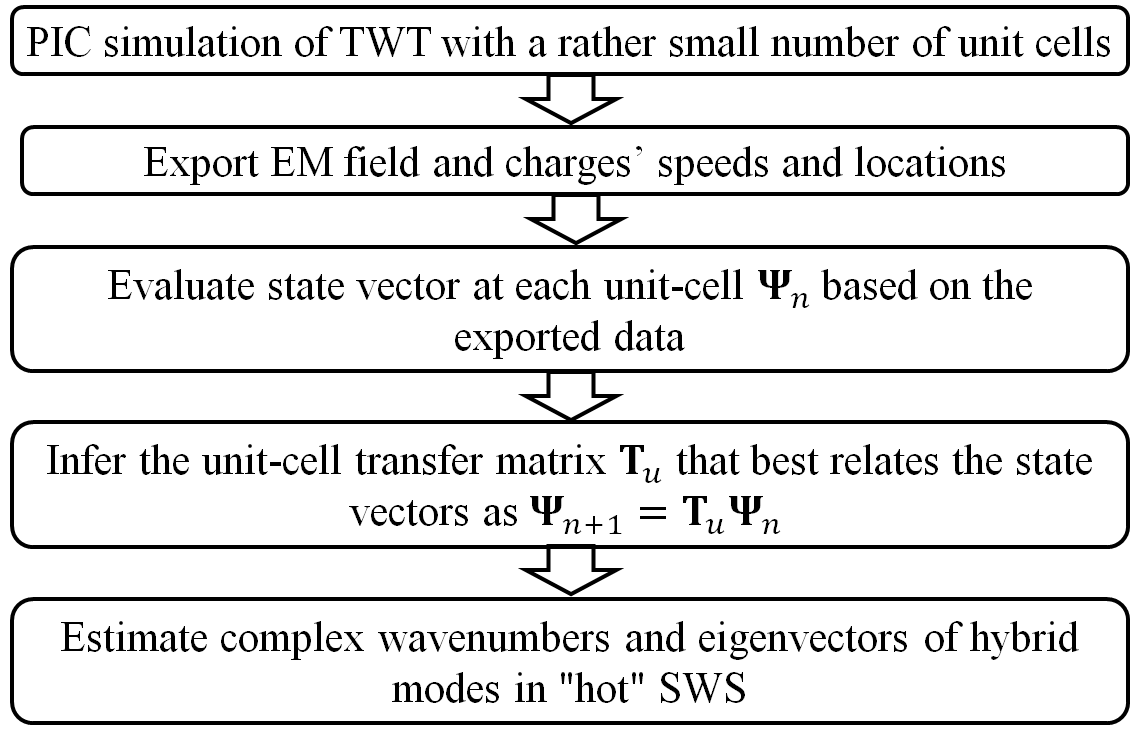
In this paper, we present a method to model TWTs by finding the equivalent transfer matrix of a unit-cell based on accurate PIC simulations of a SWS with a relatively small number of unit-cells, which is not very time consuming. The advantage of extracting the SWS unit-cell transfer matrix is not only to infer the characteristics of the hybrid modes of the EM-beam interactive system (the main goal of this paper) but also to predict the behavior of longer structures without need to simulate it using PIC (left to future investigations). To date, no commercial software provides an eigenmode solver for hot SWSs taking into account the interaction with the electron beam and losses and the accurate geometry of the SWS.
The method shown in this paper is based on finding the unit-cell transfer matrix through the interpretation of data extracted from PIC simulation for relatively short SWSs. We show that the method is used to approximately calculates the complex wavenumbers of the hybrid modes supported in a hot SWSs. The method also provides the contribution of the EM wave and spatial charge wave to each specific hybrid mode associated to each of the complex modal wavenumbers. The proposed solver is based on accurate PIC simulations of finite length hot SWSs and takes account of the precise SWS geometry, materials’ EM properties, electron beam cross-section area, confinement magnetic field and space charge effect. The proposed solver is based on monitoring both the EM fields and electron beam dynamics in each unit cell and then find the best transfer matrix that describe how the hybrid EM field-electron beam propagates along the TWT as shown in Fig. 1. Some simplifying assumptions are made, like linearity of EM and space charge waves excited in the TWT, and the electron beam is assumed not to lose energy while it travels along the TWT as discussed in the next section. Notably, the method provides the dispersion diagram of complex valued wavenumbers versus frequency of all the hybrid modes supported in the interactive hot SWS.
II Theoretical framework
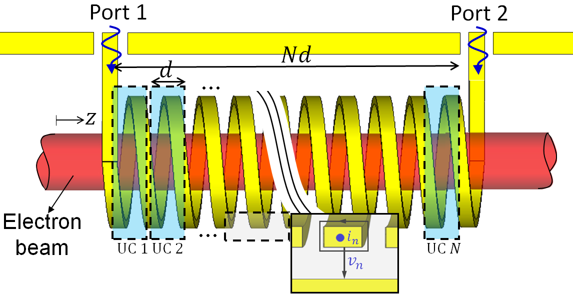
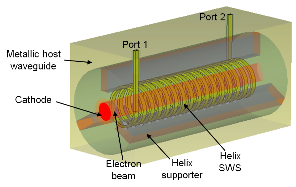
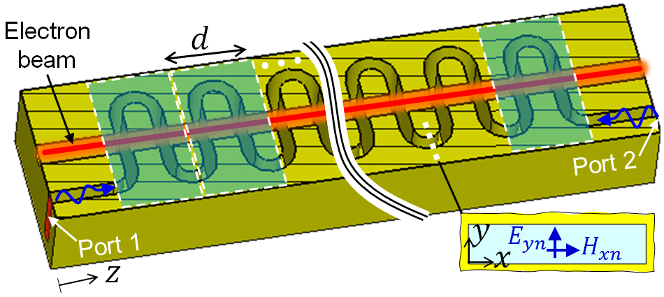
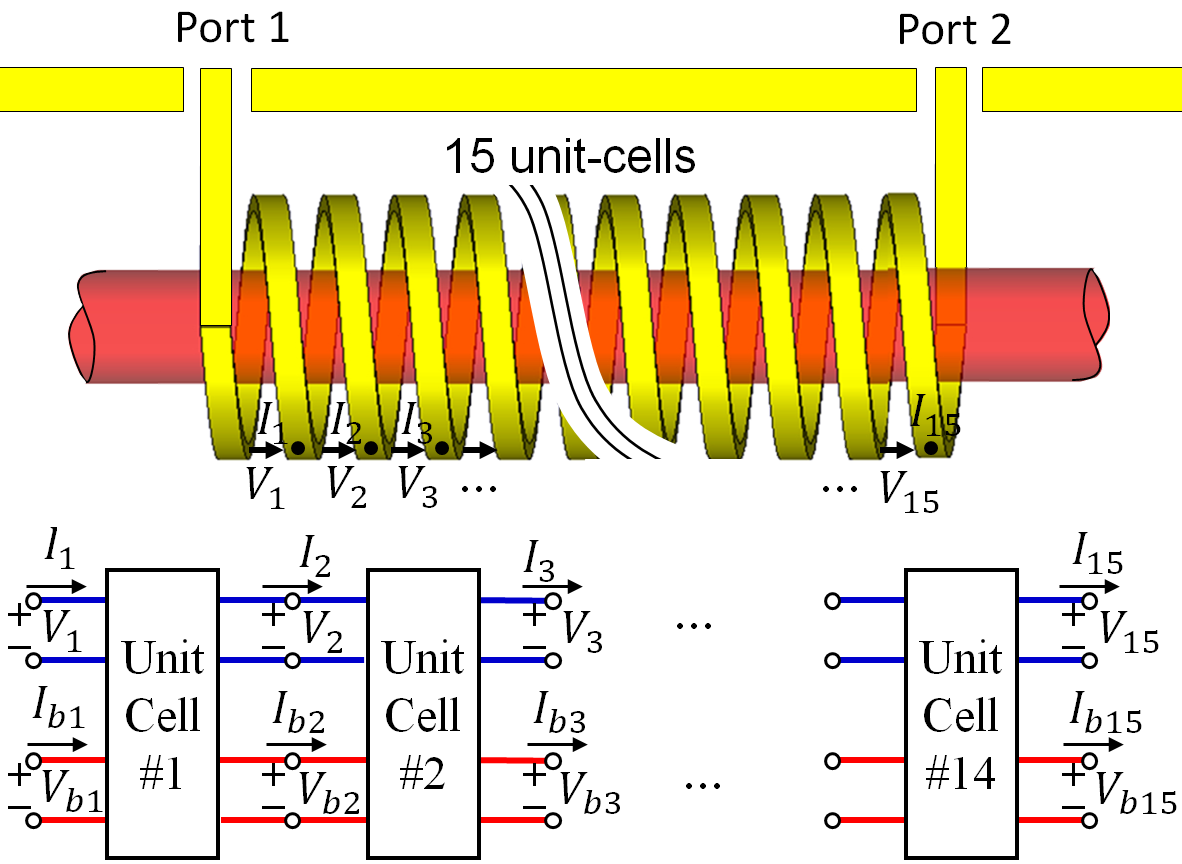
We demonstrate the performance of the proposed eigenmode to be periodically repeated solver by considering, as an illustrative example, the TWT made of a helix SWS with period consisting of unit-cells shown in Fig. 1. The input and output radio frequency (RF) signals of the structure are defined as Port 1 and Port 2. However, in the following both will be used as inputs in order to find the complex wavenumbers of the hybrid modes. It is important to point out that the following technique is general and can be applied to any kind of SWS, hence not only to helix-based SWSs. The PIC solver simulates the complex interaction between the guided EM wave and electron beam using a large number of charged particles and it follows their trajectories in self-consistent electromagnetic fields computed on a fixed mesh.
II-A Assumptions
The goal is to estimate the wavenumbers and composition of the hybrid modes of the interactive system made of EM field and the electron beam in a TWT amplifier as the one in Fig. 1. The method is based on finding the modes supported by the periodic distribution of equivalent networks shown in Fig. 1. Each unit cell is modeled using a transfer matrix which is calculated, as explained in this section, based on the results of accurate time domain PIC numerical simulations of the guided EM field interacting with the electron beam. The PIC method isbased oncharged particles motion equations and EM fields, discretized in space and time. Therefore, the EM field satisfies a discretized form of the time-domain Maxwell equations, and the PIC simulator accounts for the precise geometry and materials of the SWS and for the EM boundary conditions on the lateral walls of the periodic waveguide. Once time domain data are extracted from a PIC simulator, hybrid modes are found by imposing periodic boundary conditions along the TWT longitudinal direction z in the phasor domain using the periodic distribution of equivalent unit cell networks in Fig. 1, as discussed later on in this section. Therefore, the method estimates the complex wavenumbers of the hybrid EM-beam modes that exist in the infinitely-long sequence of equivalent unit cell networks in Fig. 1 by elaborating the data provided by the PIC method, simulating the EM field interacting with electrons in a realistic TWT of finite length. In Fig. 1 we show the data flowchart used to accomplish this task: the time domain data extracted from PIC simulations of relatively short SWSs are transformed into phasors and then used to find the unit-cell transfer matrix of which we find the eigenvalues and eigenvectors as described in this section.
In using and elaborating the data provided by the PIC solver, we make the following assumptions. Although a PIC solver calculates the speeds of discrete charged particles, we represent the longitudinal speed of all electron-beam charges as a one dimensional (1D) function . This is achieved by averaging the speed of the charges at each z-cross section as described later on. Therefore, the electron-beam velocity and density are described by the functions , and , where and are the velocity and the density of the electrons in the unperturbed beam (i.e., the dc parts), and and represent their modulation functions. In what follows, the structure is excited by monochromatic EM signals, hence we assume that the beam modulations and are also monochromatic. We also assume that the ac modulation of the electron beam is small compared to the dc part, therefore the electron beam current is well approximated by the function , where is the dc value and is its time harmonic modulation, hence we neglect non linear effects. These assumptions are the same as in the Pierce model [10, 11], but the ac values are here calculated using averaging of results taken from time-domain PIC simulations as described later on in this section. All the calculations are based on the steady state regime in a TWT, therefore the time domain signals calculated by PIC are transformed into phasors thanks to the assumption that every ac quantity is sinusoidal.
We assume that the EM fields in the hot SWS of finite length are represented in phasor domain as superposition of modes of the infinitely-long hot SWS as
| (1) |
where and are the electric and magnetic fields of the hybrid mode in the infinitely-long hot structure and they are assumed to be represented as a summation of Floquet spatial harmonics as
| (2) |
indeed they are sampled with a spatial period d along the SWS. Our goal is to find the complex-valued wavenumbers and the eigenvectors of the hybrid beam-electromagnetic eigenmodes of the infinitely-long “hot” structure using PIC simulations of the finite-length structure. The discussion in the rest of the paper is based on linearity of the system with respect to the ac EM and space charge waves, and on the assumption that the electron beam does not lose energy along its travel along the TWT, therefore the dc electron beam velocity is kept constant along the TWT. This assumption is important because we assume that the transfer matrix describing each periodic cell is the same along the whole SWS length.
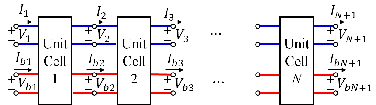
The physical quantities that represent the EM modes in the interacting SWS are electric and magnetic fields and which are represented in terms of equivalent voltages and currents and at discrete location of the periodic structure, where is the unit cell index number. In the rest of the paper we assume that only one cold EM mode is able to propagate in each direction of the cold SWS, hence only a single pair will be sufficient to describe the EM wave. Although these quantities cannot be uniquely defined in most kinds of waveguides, it is possible to define them and use them to model the space and temporal dynamics in a waveguide [28, 29, 30]. The space charge wave is represented by equivalent ac kinetic voltages and beam currents and , respectively, using the averaging method in Fig. 2 as described next. We define a state vector that describes the EM and space-charge waves at locations as
| (3) |
In the following sections we explain how this state vector is calculated using PIC calculations at locations along the SWS. Since we assume that at steady state all the quantities involved in the state vector are monochromatic, we define a state vector in phasor-domain as
| (4) |
assuming an implicit time dependence.
In the phasor domain we assume that the longitudinal propagation of the state vector satisfies the equation , where is the periodic unit cell transfer matrix, which is unknown and assumed invariant along the periodic cells of the SWS. As explained next, the first goal is to provide a method to estimate the transfer matrix . Then, we assume that each of the hybrid EM-charge wave mode in (1)-(2) is described by a state vector variation as , where is the complex wavenumber of such a mode. The goal of this paper is to find the complex wavenumbers of all the hybrid modes in the hot SWS and to find the EM and beam modal weights in (4) for each of the hybrid modes. The goal is achieved by solving the eigenvalue problem
| (5) |
once the estimate of the transfer matrix has been calculated as described in the next two sections.
II-B Determination of the system state-vector
For the particular illustrative example shown in Fig. 1, we define the voltage as the electric potential difference between helix loops and the host waveguide, as a function of the electric field via , where the index here represents the unit-cell and is the incremental vector length along the path between the helix loop and the host waveguide in the unit-cell as shown in Fig. 3. An alternative way to define the voltage for the helix is presented in Appendix A. The current that equivalently represents the EM mode can be defined as the physical current flowing in the helix tape wire which is determined from the magnetic field using the integral , along the path around a helix wire of the unit-cell as shown in Fig. 1 (using the projection of this current along the z direction leads to the same result). It is important to point out that equivalent voltage and current representing the electric and magnetic fields can be similarly defined also for other SWSs (such as serpentine waveguides, overmoded waveguides, etc.) using the equivalent field representation described in [30, 29].
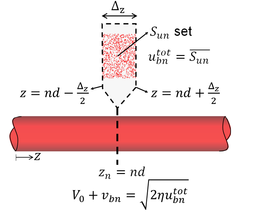
The PIC solver provides the speeds and locations of all the charged particles used to model the electron beam at any time . We define two dynamic sets that involve the speeds and coordinates of all the charges in PIC simulation at anytime instant as and , respectively, where is the total number of charged particles used by the PIC simulator to model the electron beam at time instant . The space-charge wave modulating the electron beam is assumed to be represented using two physical quantities: the electrons speed which is expressed in term of the beam equivalent kinetic voltage , and the space-charge wave current modulation , as also described in Refs. [31, 32, 11]. The beam total equivalent kinetic voltage at the entrance of the unit-cell is defined as where is the equivalent speed of the space-charge wave calculated as the average of the speeds of the set
| (6) |
that is defined by all the charged particles that are in vicinity of the entry of the unit-cell (), and within the small spatial interval , as illustrated in Fig. 2. The length of the spatial interval is chosen to be very small, i.e, , where , and is the electron time-average speed and is the frequency modulating the space-charge wave. Although is chosen to be small, it should be also large enough to contain a very large set of charged particles, as illustrated in Fig. 2. The charge-wave current at the unit-cell () is defined as , where is the electron beam charge density at the entry of the unit-cell and is calculated as where is the charge value of each PIC-defined particle and is the number of such charged particles in the set . The ac modulated parts are then calculated as and which are used later on to construct the system’s state vector. As described below, when we calculate the phasor associated to we will retain only the frequency component at radian frequency and not the higher order harmonics.
It is important to point out that in this illustrative example we assume that the SWS supports one cold EM mode that can propagate in each direction and that the electron beam is represented by a single state that describes the average behavior of the speed and density of the charged particles distribution. Describing the EM-chanrge wave state using the four-dimensional state vector (3)constitutes a good approximation in many cases where the SWS supports only one EM mode (in each direction) and the electron beam is modulated in a homogeneous way, i.e., the beam modulation does not change with radial and azimuthal angular directions. However, a more accurate model of the hot SWS could be obtained by using an equivalent multi-transmission line model to describes all the EM modes in the SWS, and an equivalent multi “beam transmission line” (or multi stream beam) to describe the electron beam. Indeed, since we know that in reality the momentum and charge density description of the electron beam dynamics usually looks like a multi-valued function, it may be convenient to decompose the electron beam using various areas in transverse cross section leading to a multi “beam transmission line” with multiple kinetic voltages and space-charge wave currents. For the sake of simplicity, in this paper the electron beam dynamics is represented only with one “beam transmission line”, i.e., with a single () pair.
The interaction between the space-charge wave and the EM wave yields three eigenmodes that travel in the beam direction in addition to a mode (mainly made of only EM field) propagating opposite to the beam direction, indeed the latter has very little interaction with the electron beam [11]. The three hybrid modes with positive phase velocity are composed of both EM fields and space-charge wave modulations, and form the “three-wave” model used in Refs. [33, 11]. Under the assumption of using a single tone excitation of an EM wave from Port 1 and/or Port 2, all four hybrid EM-charge wave modes in the interacting system can be excited: an excitation from Port 1 mainly excites the three interacting hybrid modes, whereas the excitation from Port 2 excites mainly the EM mode propagating in opposite direction of the beam. Reflections may occur at the left and right ends in a realistic finite-length SWS, so in reality all four modes may be present, depending on the EM reflection coefficients at the two ends.
At steady state, the state vector is represented in phasor-domain as in (4), assuming an implicit time dependence for all physical quantities. The phases of phasors are calculated with respect to a fixed time at steady state. The phasor-domain representation (4) of the state vector is calculated as
| (7) |
where and is a time reference used to calculate the phasors and it should be greater than the steady state time, i.e., It is important to mention that only the fundamental component at frequency is maintained after the Fourier transform is carried out to build the state vector in phasor domain in (4), hence all frequency harmonics in are neglected in the following. Lower case letters are used for the time-domain representation whereas capital letters are used for the phasor-domain representation. In the phasor-domain, we model each unit cell of the interacting SWS as a 4-port network circuit with voltages and currents representing both the EM waves and the electron beam dynamics, as shown in Fig. 1. As described in the previous section, under the assumption of small signal modulation of the beam’s electron velocity and charge density, the 4-port networks modeling the EM-charge wave interaction in each unit-cell of the hot SWS are assumed identical. Therefore, one can define a transfer matrix of the interaction unit-cell of a SWS using the relation between the input and output state vector at each unit-cell as
| (8) |
where and are the input and output state vectors of the unit-cell, respectively, where n = 1, 2,.. N. The state vectors are calculated from using PIC simulations; then an estimate of the transfer matrix is inferred by the method described in the following section.
II-C Finding the transfer matrix of a unit cell of the interactive system
II-C1 Approximate best fit solution
The relations in (8) represent linear equations in unknowns which are the elements of the transfer matrix . The system in (9) is mathematically referred to as overdetermined because the number of linear equations ( equations) is greater than the number of unknowns (16 unknowns). We rewrite (8) by clustering all the given equations in matrix form as
| (9) |
where
| (10) |
is a matrix and its columns are the state vectors at input of each unit-cell, and
| (11) |
is an analogous matrix but with a shifted set of the state vectors, i.e., its columns are the state vectors at the output of each unit-cell. Our first goal is to find the 16 elements of the transfer matrix .
An approximate solution that best satisfies all the given equations in Eq. (8), i.e., minimizes the sums of the squared residuals, is determined similarly as in [34, 35, 36] and is given by
| (12) |
It is important to point out that all the four modes of the interactive EM-charge wave system should be excited to be able to have four independent columns in the construction of the matrices and since we need apply the inverse operation in (12). This occurs when there is sufficient amount of power incident on Port 1 and Port 2.
II-C2 Distinct determined solutions
The transfer matrix can also be determined directly by taking any four equations of Eq.(8), assume we choose Eq. (8., Eq. (8., Eq. (8. and Eq. (8., and therefore yields
| (13) |
where
| (14) |
and
| (15) |
Assuming the SWS has unit cells, there will be possible solutions for , where is the number of the combinations to choose and out of choices. Under the assumption that the transfer matrices of each unit-cell are identical, the sets of four eigenvalues resulting from the solutions of should be identical too. However, the electron beam non-linearity and other factors may cause small discrepancy in the eigenvalues resulting from the various eigenmode solutions of , as shown in the next section.
It is important to point out that some combinations may result in a underdetermined system where the rank of could be less than 4, i.e., could be singular. For example, when selecting unit cells toward the right end of the TWT (e.g., and ), the state vectors forming are dominated by only one mode that has exponential growing in direction, and therefore the matrix tends to be singular. Therefore, one can neglect combinations that are close to be singular by checking the determinant of for each combination. Following this method, multiple transfer matrices are found that lead to multiple wavenumbers that are clustered around four complex values.
II-D Finding the hybrid eigenmodes of the interactive system
Once the transfer matrix is estimated (either using the best-approximate solution of the overdetermined system or determined solutions ), the hybrid eigenmodes are determined by assuming a state vector has the form of , where is the complex Bloch wavenumber that has to be determined and is the SWS period. Inserting the assumed sate vector z-dependency in (8) yields the eigenvalue problem in (5). Note that eigenvalues and eigenvectors of the eigenvalue problem in (5) depend only on the transfer matrix . The four eigenvalues,
| (16) |
of the transfer matrix lead to four Floquet-Bloch modes , where , with harmonics , where is an integer that defines the Floquet-Bloch harmonic index as in (2). Some examples are provided in the next sections. Note that (5) provides also the eigenvectors and important information can be extracted from them. Each eigenvector possesses the information of the respective weights of the EM field () and space-charge wave () in making that particular hybrid eigenmode solution. Furthermore, including the case when more EM modes are used in the SWS interaction zone or when two hybrid modes concur in the synchronization, an analysis of the eigenvectors can also show possible eigenvector degeneracy conditions. For example, in [37, 38, 39], two hybrid modes are fully degenerate in wavenumbers and eigenvectors forming what was called a “degenerate synchronization” (degeneracy between two hot modes). Other important degeneracy conditions are those studied in [40], where three or four fully degenerate EM modes in the cold SWS are used in the synchronization with the electron beam, a condition refer to as “multimode synchronization” (degeneracy among cold EM modes).
In a finite length TWT, the total EM field (represented by , ) and space-charge wave (represented by , ) resulting from their interaction, calculated at each location, are represented in terms of the four eigenmodes,
| (17) |
where is the weight of the mode, which depends on the mode excitation and boundary conditions, and is the interactive system eigenvectors obtained from (5). Each Floquet-Bloch mode in the periodic hot SWS is represented as .
In this paper we show how to determine the eigenvector and wavenumber of each of the four hybrid eigenmodes (), using two illustrative examples: a centimeter wave (i.e., “microwave”) and a millimeter wave TWT amplifier.
III Application to a helix-based TWT amplifier
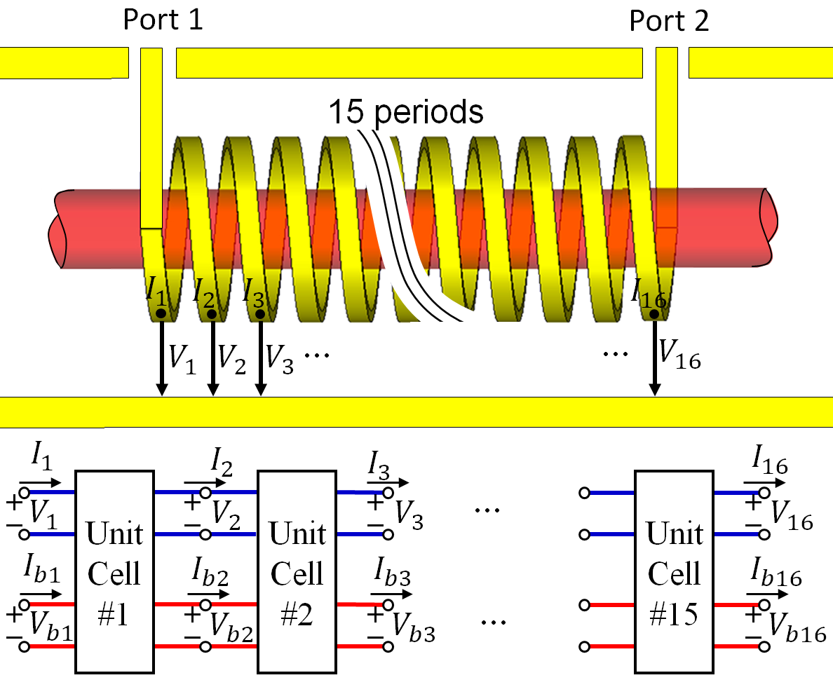
We demonstrate how the technique described in the previous section is applied considering an illustrative example made of a C-Band TWT amplifier described in [41] and shown in Fig. 3. Such TWT amplifier operates at 4 GHz and uses a solid linear electron beam with radius of 0.63 mm, with dc kinetic voltage of 3 kV and dc current of 75 mA. The axial dc magnetic field used to confine the electron beam is 0.6 T. The TWT uses a copper helix tape with inner radius of 1.26 mm and period of 0.76 mm, and the metallic tape has mm thickness and mm width. The metallic circular waveguide has radius of mm and the three supports that physically hold the helix are made of Anisotropic Pyrolytic Boron Nitride (APBN) with relative dielectric constant of 5.12 and and with width of mm. The numerical simulation consists of 15 periods of the structure. We show the numbering scheme used to define the voltages and currents representing the EM wave and the space-charge wave at the begin and end of each unit-cell in Fig. 3. While the whole structure is considered in PIC simulations, when we apply the proposed method we do not consider the first and the last state vectors (i.e., at the beginning and end of of the first and last unit cells) because the begin and the end of the SWS are close to the coaxial waveguide input and output ports, and higher order modes due to the transformation of the TEM wave in the coaxial waveguide into the SWS modes would influence the calculation of the unit-cell transfer matrix.
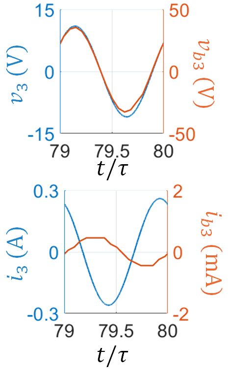
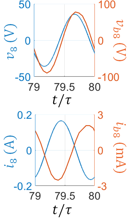
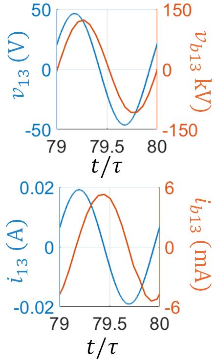
First, we study the system eigenmodes at single frequency by exciting Port 1 and Port 2 with 10 Watt and 5 Watt, receptively, at 4 GHz. Note that indeed, even if the actual TWT operation involves feeding from one side only, the scheme explained in the above section may need a SWS feed from both the left and right ports to be sure we excite all the modes. It is important to mention that changing the power levels at Port 1 and Port 2 shall not significantly affect the resulting eigenmode solution as long as the power levels are not too high to involve non-linear regimes. The total number of charged particles used to model the electron beam in the PIC simulation is about whereas the whole space in the SWS structure is modeled using mesh cells. Once steady state is reached, the time-domain state vector is monitored at each unit-cell. Figure 4 shows the four components (3) of the state vector at the , and unit cells in the time interval between and , where ns is the time period at 4 GHz. The phasor-domain representation (4) of the state vector is calculated using (7) with ns.
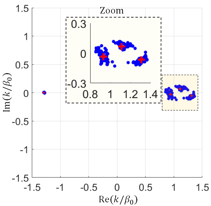
The four wavenumbers of the eigenmodes of the interacting SWS system are shown in Fig. 5 based on results from Eq. (9) leading to the four red crosses, and from Eq. (13) leading to the various blue dots. The scattered blue dots represent 75 sets of four complex wavenumbers associated with 75 sets of transfer matrices obtained from Eq. (13) using 75 combinations of and to give the highest 75 determinants of the matrix out of the all 330 combinations. It is important to mention that the solutions associated with the rest 255 combinations and were ignored because they result in almost singular matrices and .
The results in Fig. 5 show a good agreement between the red crosses that represent the four wavenumbers obtained from the eigenvalues of where is the best-approximate solution of the overdetermined system in (9) and the blue dots that represent the eigenmodes of various estimates of obtained from solutions of (13). It is important to point out that the small deviations between the complex wavenumbers obtained from different solutions is due to non-idealities resulting in having non-identical unit-cells along the structure. This may happen due to the electron beam non-linearity and the change of the beam kinetic voltage along the TWT, in addition to the errors due to finite mesh and finite number of charged particles used to model the TWT dynamics. The resulting eigenmodes are qualitatively in good agreement with the expected description using the theoretical transmission line-based Pierce model [11] that basically says that there exist three wavenumbers with positive real part, and one of them has positive imaginary part which describes the amplification of the EM wave along the SWS.
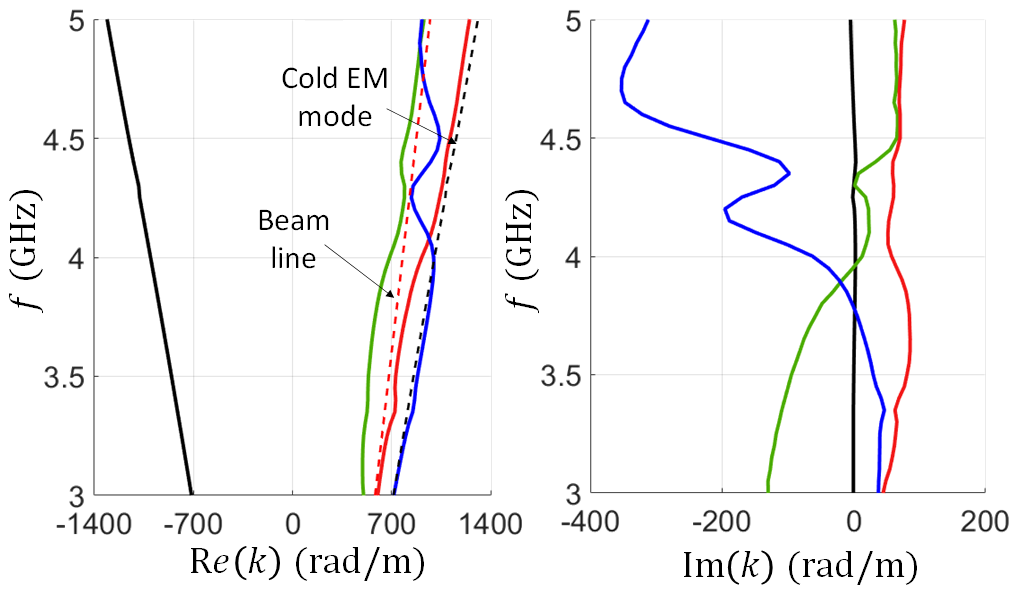
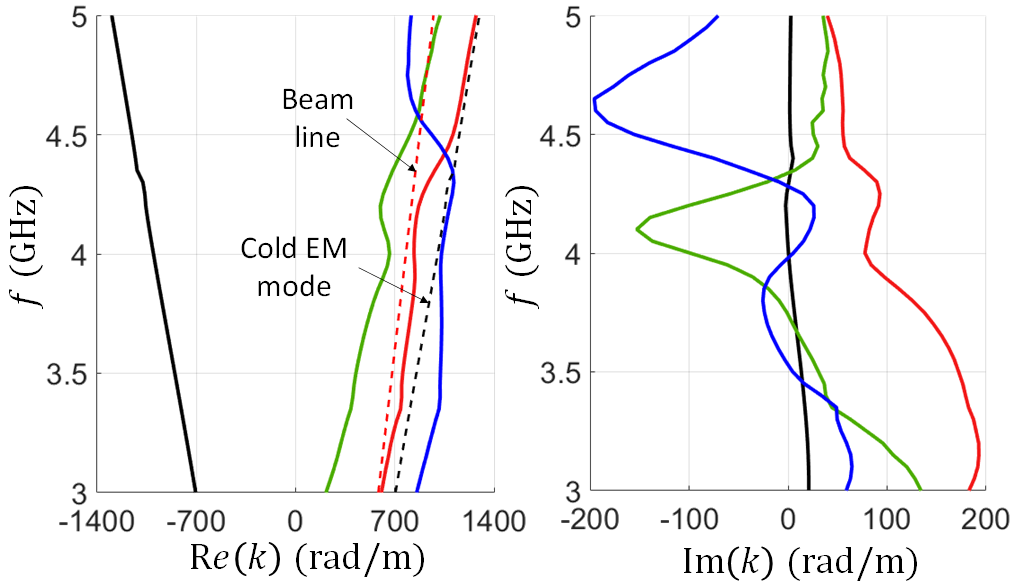
The wavenumber-frequency dispersion describing the eigenmodes in the hot SWS is determined by running multiple PIC simulations at different frequencies and then determining the transfer matrix of the unit-cell at each frequency using Eq. (9), i.e., the result shown by the red crosses. In other words we repeat the red-cross results shown in Fig. 5 at various frequencies. The dispersion diagram of the four modes in the hot EM-electron beam system is shown in Fig. 6 (solid lines) using 42 frequency points (42 PIC simulations). The dashed red and blue lines represent the space-charge wave (i.e., the beam line) and EM modes when they are uncoupled (i.e., in the “cold” case). The dispersion of the EM mode in the cold SWS (dashed black) is found by the finite element method-based eigenmode solver implemented in CST Studio Suite by numerically simulating only one unit-cell of the cold helix SWS.
The black solid line in Fig. 6 is the hybrid mode propagating with <0, i.e., in opposite direction of the beam flow and basically no beam-EM interaction occurs, and it is made mainly of EM field as also explained later on in Fig. 7. Indeed, as compared to the cold EM modes, the solid-black line of the hot SWS simulation is superposed to the dispersion line of the cold EM mode propagating in the negative -direction.
The three eigenmodes with wavenumbers with positive real part (solid red, green, blue lines) are the eigenmodes affected by the interaction between the electron beam’s space-charge wave and the EM wave propagating in the same direction. The solid-red curve in the dispersion relation has >0 and represents the growing eigenmode that causes the amplification of the EM wave. The imaginary part of the growing mode starts to decreases with increasing frequency because the difference between the speed of the space-charge wave and that of the EM wave in the SWS (when we consider them uncoupled) increases. It is important to mention that a single PIC simulation could also be investigated to find the dispersion relation when using a moderately wide-band gaussian pulse at the input ports, however it would require excessive post processing to be able to decompose each tone behavior and it does not fully account for steady state regime resulting from the interaction with the electron beam that would otherwise includes also non-linear effects.
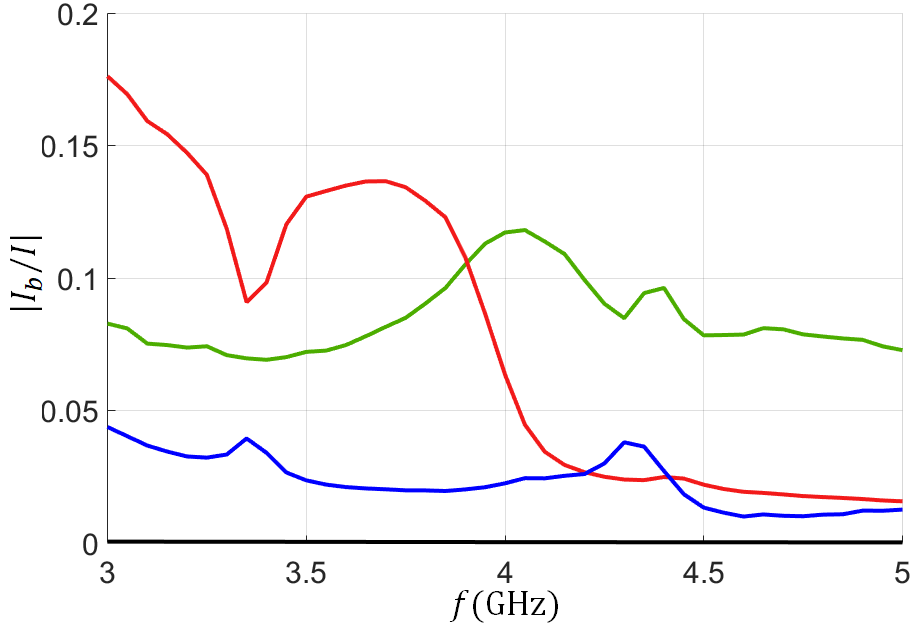
The hybrid modes describing the EM-charge wave interaction are further understood by looking also at their eigenvectors, besides their wavenumbers. Eigenvectors satisfy Eq. (5) and are the same used in the aforementioned discussed method to find the transfer matrix. The eigenvectors components in (4) describe the relative weight of the EM wave (, ) versus the space-charge wave , , for each of the four modes , with m = 1,2,3,4. The relative strength of the EM wave and space-charge wave in each eigenmode is determined in Fig. 7 by calculating the ratio between between the ac electron beam current and the EM mode equivalent transmission line current. The ratio for each of the four eigenmodes is shown using colors consistent with those in Fig. . The figure verifies that the eigenmode with EM wave propagating with <0 (solid-black line), in the direction opposite to the electron beam flow does not interact with the electron beam since the beam ac current component associated to this mode is vanishing. The growing eigenmode (>0), red line, is the one responsible of EM amplification and it shows a good EM-charge wave interaction from 3.6 GHz to 4.2 GHz which is in agreement with the bandwidth specification of the amplifier given in [41]. Indeed, the operation of TWT as an amplifier depends on having a spatially growing mode (along the SWS) and the only mechanism to have a growing mode is via the coupling to the electron beam that gives back power to the EM wave after electron bunching is formed. This plot indeed shows that the red mode is the result of synchronization and generate a very strong electron beam.
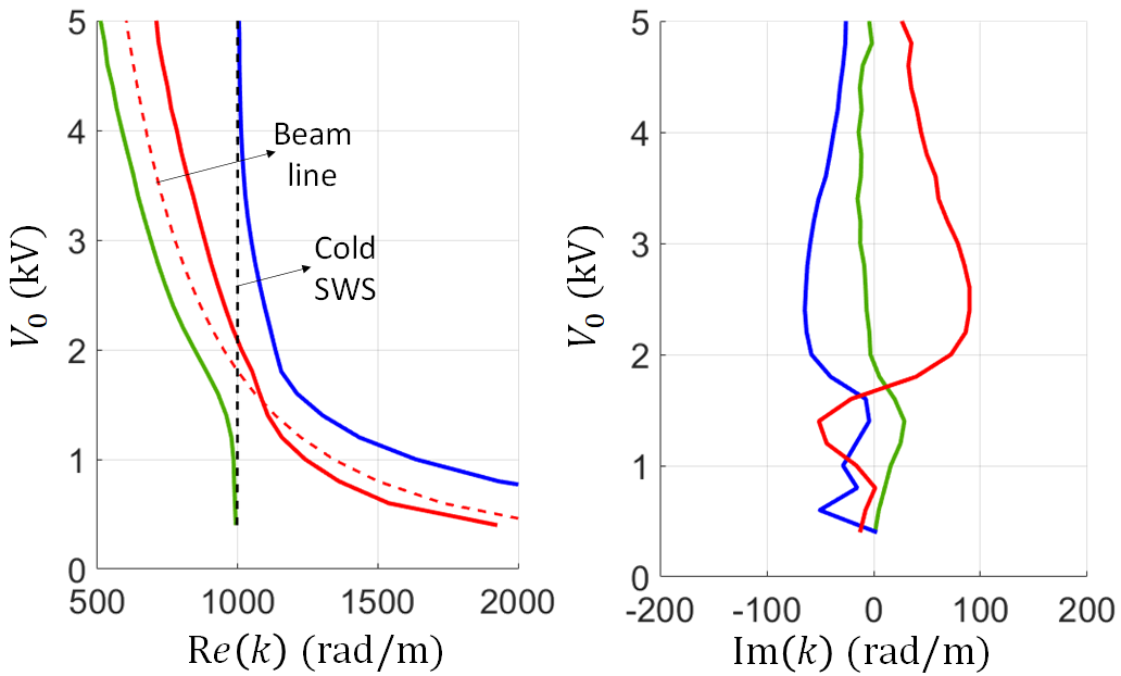
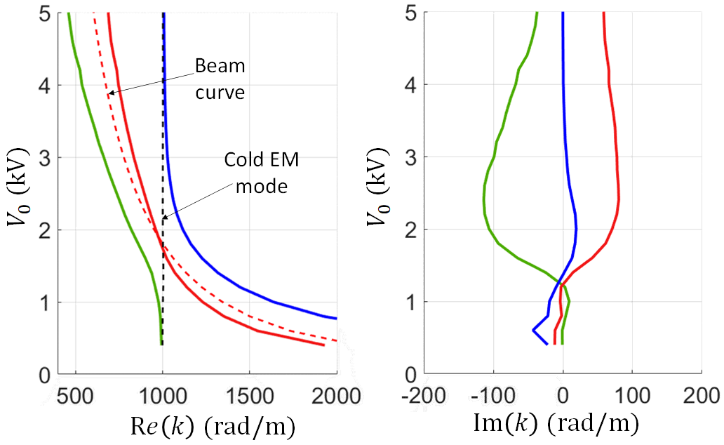
A synchronization study is performed by observing the modes’ complex wavenumber when sweeping the beam dc voltage. In Fig. 8 we show the wavenumbers for the three hot eigenmodes with positive real part (red, green, and blue curves) when changing the beam dc kinetic voltage while the dc beam current is maintained at 75 mA, at a constant frequency of 4 GHz. Solid lines represent the three eigenmodes in the interactive (i.e., hot) SWS, whereas the dashed lines represent the beam line (red dashed) and the cold EM mode with positive wavenumber (i.e., in the cold SWS). Since the frequency is fixed the cold EM mode has a fixed wavenumber 999.8 and it is described by the vertical black-dashed line. The phase velocity of the EM mode in the cold SWS is since rad/s, where m/s is the speed of waves in free space. Synchronization occurs approximately in the region where the two dashed lines, beam line and EM-wave line, have the same wavenumber, i.e., the same phase velocity, which happens just above 1.8 kV. The TWT amplification factor, mainly represented by the positive imaginary part of the red eigenmode, shows a peaking around synchronization point of 1.8 kV which is corresponding to a beam speed , where is the charge to mass ratio of the electron.
At lower or much higher dc voltage with respect to the synchronization point would make the beam-EM interaction is weak. This is also understood by noting that the gain starts to decay away from the interaction voltage region and the hot modes (resulting from the interaction) tend to overlap with the cold modes (without interaction) away from such region. In particular at low frequency the solid green curve tends to overlap with the cold EM mode, whereas at high frequency the solid blue line tends to overlap with the cold EM mode. The two solid red and blue curves at low dc voltage tend to overlap with the beam curve (red dashed), whereas the two solid red and green curves at high voltage tend to overlap with the beam line (red dashed): therefore these hot modes tend to overlap with the beam line (non-interactive beam) at high and low voltage despite some shifts which may be due to space charge effects. Near the synchronization point, the splitting of the solid green and blue curve (versus the red curve that does not split) represent the strong interaction between the electron beam and the EM field.
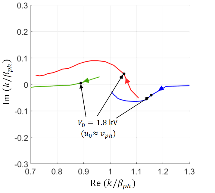
In Fig. 8 we show the complex plane mapping of the wavenumbers for the three hot eigenmodes with , shown in Fig. 8, varying the electron beam dc voltage (i.e., the speed of the electrons ). The black dots represent the interactive modes wavenumbers when the beam dc voltage is kV which results in an electron beam with average speed very close to the EM mode in the cold SWS, i.e., close to the synchronization point . The complex wavenumber location of the three interactive modes shown in Fig. 8 is in agreement with the three-wave theory of the Pierce model [33, 11] around the synchronization point. When , there are three modes with >0: two of them are waves that are slower than the electron beam average speed , and among these two, one wave is growing in the beam direction while the other one is decaying. The third mode is basically an unattenuated wave that travels faster than the beam-average speed .
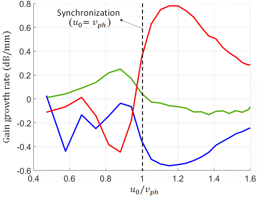
The power flow for each mode of the hot (i.e. interactive) SWS is written in the form of [42], where is the initial amount of power carried by the same mode at . We define the power gain resulting from the interaction between the EM and space-charge wave for as Thus gain growth rate for each mode is dB/m. In Figure 9 we show the gain growth rate for the three interactive modes (those with ) versus electron-beam charges average speed (normalized by the cold SWS phase velocity , where is the wavenumber of the EM mode in the cold SWS). The figure shows that there is an optimal point for the interaction (where ) which is very close to synchronization point where the power transfer from the kinetic energy of the electron beam into RF power in the SWS is maximum, as discussed in [43, 10]. The figure also show that the largest power transfer, from the kinetic energy of the electron beam into RF power, occurs when the average speed of electron beam charges is roughly above the speed of the cold EM wave in the SWS.
In Appendix A we show the effect of changing the voltage definition and the SWS length on the eigenmode calculations for the same helix SWS considered in this section. There, we define the voltages representing the EM waves as the potential differences between each two successive helix loops. Results are qualitatively in agreement with what described here, and only small quantitative differences are observed.
IV Application to serpentine-based TWT amplifier
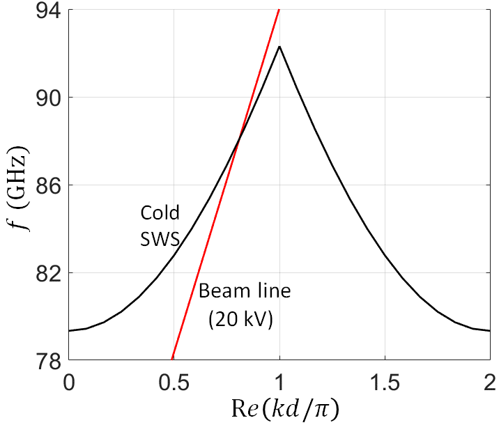
We demonstrate the utility of the proposed eigenmode solver method to find the eigenmodes in the hot serpentine SWS operating at a millimeter wave band. The interaction with the electron beam is periodic and not uniform as for the case of the helix SWS. Serpentine SWSs have recently gained a lot of interest due to the growing importance of millimeter wave and terahertz frequencies in modern applications and also due to the advancement of fabrication technologies such as LIGA (LIthographie, Galvanoformung, Abformung). As an illustrative example, we use the same geometry of serpentine SWS discussed in [44, 45], as shown in 10. The serpentine waveguide is made of copper and has rectangular cross-section of dimensions mm and mm, bending radius of mm (radius at half way between inner and outer radii), straight section length of 0.6 mm, beam tunneling radius of mm. The TWT comprises 13 unit-cells . An electron beam with dc voltage kV is used such that the synchronization occurs with a forward EM wave leading to amplification. In Fig 10 we show the beam line (red line) where , and the dispersion diagram of EM modes in the cold SWS (black line). Synchronization, , between the electron beam and the forward EM wave occurs at frequencies centered at GHz.
Figure 10 shows the setup used for PIC simulations. We consider the electron beam to have a radius of 0.13 mm, a dc current of A and an axial confinement dc magnetic field of 0.6 T. Our goals is to obtaining the dispersion of the hot serpentine SWS, i.e., the complex wavenumber of the hybrid modes that account for the interaction between the electron beam and the EM wave. In our method we excite the SWS from Port 1 with 10 Watts and from Port 2 with 5 Watts. An amplifier has the input at one port and the output at the other one, but here we want to excite the supported eigenmodes sufficiently to be observed in the calculations. The serpentine supports the mode which is the only one propagating in the rectangular waveguide. Since the serpentine waveguide does not support a TEM mode, voltage and current cannot be uniquely defined. We use the equivalent representation in [28, 30, 29] that models the waveguide as a transmission line with equivalent voltage and current. Following the derivations in [28, 30, 29] for the mode in a rectangular waveguide, the transverse fields are written as
| (18) |
Using (18), the discrete voltages and the currents that represent the EM state at different rectangular cross-sections of the serpentine waveguide are found as
| (19) |
where and are the traverse electric and magnetic fields calculated at the center of the rectangular ( and ) waveguide cross section as shown in the inset in Fig. 10 and they are calculated at the unit cells boundaries shown in Fig. 10.
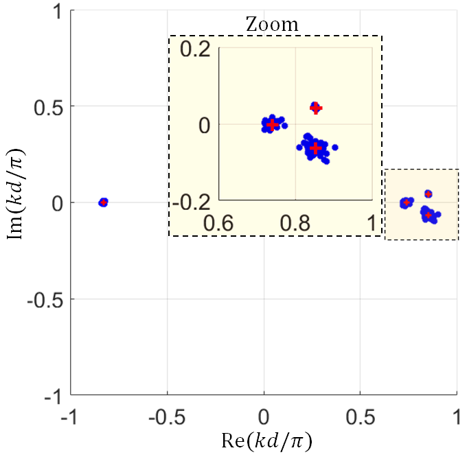
We start by studying the eigenmode wavenumbers in the interacting SWS system at constant frequency GHz, which is very close to the synchronization point where . The four complex wavenumbers of the hybrid modes are shown in Fig. 11 based on results from Eq. (9) leading to the four red crosses, and from Eq. (13) leading to various blue dots. The scattered blue dots represent 37 sets of four complex wavenumbers associated the largest 37 determinants of the matrix out of the all 126 combinations. The blue dots cluster around the four red crosses, as expected. It is important to mention that we ignored the state vectors of the first and the last two unit cells to generate our results because they may involve high order modes that affect the results. The complex wavenumbers locations of the three interactive modes (those with >0) shown in Fig. 11 are in good agreement with predictions of the three-wave theory of the Pierce model [33, 11].
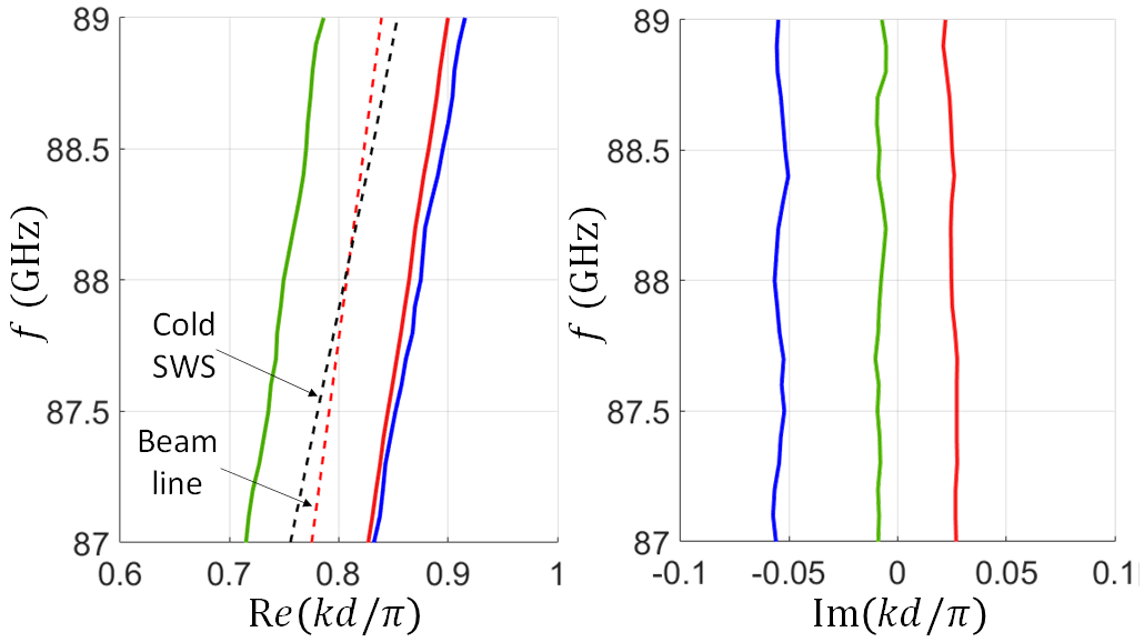
In Fig. 11 we show the modal dispersion relation accounting for the EM-beam interaction in the serpentine SWS using 21 frequency points. The hot dispersion diagrams are obtained using the best-approximate solution of the overdetermined system in (9). As in the previous section, dashed lines represent the two uncoupled systems: the beam line (dashed red) and the EM mode in the cold SWS (dashed black). The electron beam has a dc voltage of kV so the electron beam interacts with the forward EM wave resulting in an eigenmode with positive imaginary part leading to TWT amplification (red curve). We show only the three modes with positive real wavenumber. One wavenumber has positive imaginary part (solid red curve), which is responsible for amplification, whereas the other two modes resulting from the interaction are decaying and unattenuated modes, in agreement with the Pierce model [11]. The gain per unit-cell associated to the mode is defined as
| (20) |
which is equivalent to dB. The imaginary part of the wavenumber of the amplification mode (solid red) is almost constant and equal to in the frequency range from 87 GHz to 89 GHz shown in Fig. 11, because the phase synchronization condition is almost satisfied for the considered frequency band, i.e., over the shown band (relative band of around GHz) in this example. Thus, the gain per period resulting from the amplification mode (solid red) is 0.74 dB in this frequency range which is close to the small-signal gain 1 dB reported in [45] that was obtained by simulating the serpentine TWT amplifier at 90 GHz.
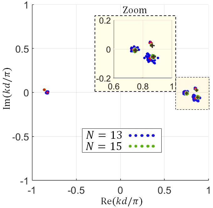
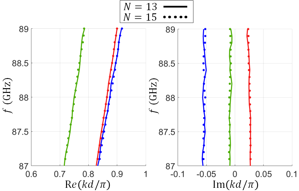
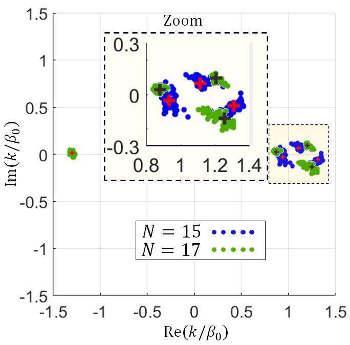
A repeatability study is performed by obtaining the dispersion relation for the serpentine hot SWS using two different numbers of unit cells (all other parameters are kept the same for the two TWT configurations as previously described). Indeed, the transfer matrix of the hot SWS unit-cell should not be a function of the used number of unit-cells, therefore, the dispersion relation obtained using different numbers of unit cells should not be affected. In Fig. 12 we show the complex wavenumberscalculated from the unit-cell transfer matrix estimated using data from PIC simulations of two SWSs with (as in the previous example) and unit cells. In each case, we plot 37 sets of four wavenumbers obtained from 37 estimated transfer matrices (distinct determined solutions): blue and green dots represent the cases with and unit cells, respectively. The plotted sets are the ones associated with the highest 37 determinants of the matrices used to determine the unit-cell transfer matrices out of the all 126 combinations for the case with unit cells and 330 combinations for the case with unit cells . The red and black crosses represent the wavenumbers obtained from the best-approximate solution of the overdetermined system for the cases with and unit cells, respectively. The clustering of wavenumbers at 88 GHz in Fig. 12 shows a good agreement between the two cases based on and unit cells. In Fig. 12 we compare the dispersion relation obtained based on the best-approximate solution of the overdetermined system (red and black crosses in Fig. 12): solid and dotted curves represent the dispersion obtained from simulating the hot SWS with and unit cells, respectively. The figure shows an almost negligible discrepancy between the dispersion diagrams obtained using two SWS lengths.
f
V Conclusion
A TWT eigenmode solver to determine the complex wavenumbers of the hybrid eigenmodes in hot SWSs (i.e., accounting for the interaction of the electron beam and the EM wave) has been demonstrated using a novel approximate technique based on data obtained from PIC simulations. The technique has been able to predict the growing mode’s complex wavenumber in both TWTs studied here based on: (i) a SWS made of a circular waveguide with a helix working in the GHz range; (ii) a SWS made of a serpentine waveguide for millimeter wave amplification. The method is based on elaborating the data obtained from time domain PIC simulations, hence accounting for the precise waveguide geometry, materials, losses, and beam space charge effects. We believe that the proposed technique is a powerful tool for the understanding and the design of TWTs amplifiers.
In the present investigation we have focused on determining the complex wavenumbers of the hybrid EM-beam modes, but the same technique can also be used to estimate the performance of longer TWTs based on simulations of shorter TWTs, i.e., it can be used in the design and initial optimization of TWTs. The determination of wavenumbers and eigenvectors of all the hybrid modes supported in a TWT amplifiers discussed here can also be useful to study mode degeneracy conditions in hot SWSs as those investigated in [37, 38, 39].
VI Acknowledgment
This material is based upon work supported by the Air Force Office of Scientific Research award number FA9550-18-1-0355 and award number FA9550-20-1-0409. The authors are thankful to DS SIMULIA for providing CST Studio Suite that was instrumental in this study.
Appendix A Helix dispersion relation using an alternative voltage definition and different structure lengths
In this appendix we test how changing the voltage definition impacts the eigenmodes calculations for the TWT made of a helix SWS considered in Sec. III. We also test how changing the length of the simulated TWT impacts the eigenmodes calculations.
A-A Changing voltage definition
The structure we study here has the same helix parameters and length as the one presented in Sec. III. The only difference is that here we define the voltages representing the EM field as the potential differences between each two consecutive helix loops. We show in Fig. 13 the definition and the numbering scheme for voltages and currents representing the EM and space-charge waves,that are used to construct the circuit network model of each unit-cell. Note that although the structure has 15 periods but it is modeled using 14 network unit-cells because the new voltage definition involve two loops of the helix as shown in Fig. 13.
Theoretically, changing the voltage definition should not impact the eigenvalues, i.e., the determination of the hot SWS modal wavenumbers, however, it affects the calculation of the eigenvectors of the system. We show in Fig. 13 and Fig. 13 the the four complex modal wavenumbers of the hot EM-electron beam system, versus frequency and beam voltage, respectively. The small discrepancy between the wavenumber obtained in Sec. III and the one obtained here based on a different voltage definition may be explained considering the electron beam non-linearity and the change of the beam kinetic voltage along the TWT, in addition to the errors due to finite mesh and finite number of charged particles used to model the TWT dynamics.
A-B Changing the SWS length
We study the effect of changing the simulated TWT length on the calculation of the four complex wavenumbers calculated from the transfer matrix estimated using data from PIC simulations of two SWSs with and unit cells. All the used parameters here are kept the same as the ones in Sec. III except that we change the number of the helix SWS unit cells to be , instead of . In Fig. 14 we show the complex wavenumbers. In each case, we plot 75 sets of four wavenumbers obtained from 75 estimated transfer matrices (distinct determined solutions):blue and green dots represent the cases with and unit cells, respectively. The plotted sets are the ones associated with the highest 75 determinants of the matrices used to determine the unit-cell transfer matrices out of the all 330 and 715 combinations for the case with and unit cells, respectively. Red and black crosses represent the wavenumbers obtained from the best-approximate solution of the overdetermined system for the cases with and unit cells, respectively. The clustering around distinct wavenumbers is consistent when considering the two SWS lengths. The small but noticeable discrepancy in values between the wavenumbers clustering for both cases may be explained as the result of the electron beam non-linearity and other factors like the electron beam loss of energy along the SWS.
References
- [1] D. F. Minenna, F. André, Y. Elskens, J.-F. Auboin, F. Doveil, J. Puech, and É. Duverdier, “The traveling-wave tube in the history of telecommunication,” The European Physical Journal H, vol. 44, no. 1, pp. 1–36, 2019.
- [2] X. Li, X. Huang, S. Mathisen, R. Letizia, and C. Paoloni, “Design of 71–76 GHz double-corrugated waveguide traveling-wave tube for satellite downlink,” IEEE Transactions on Electron Devices, vol. 65, no. 6, pp. 2195–2200, 2018.
- [3] J. H. Booske, “Plasma physics and related challenges of millimeter-wave-to-terahertz and high power microwave generation,” Physics of plasmas, vol. 15, no. 5, p. 055502, 2008.
- [4] S. Sengele, H. Jiang, J. H. Booske, C. L. Kory, D. W. Van der Weide, and R. L. Ives, “Microfabrication and characterization of a selectively metallized W-band meander-line TWT circuit,” IEEE transactions on electron devices, vol. 56, no. 5, pp. 730–737, 2009.
- [5] J. H. Booske, R. J. Dobbs, C. D. Joye, C. L. Kory, G. R. Neil, G.-S. Park, J. Park, and R. J. Temkin, “Vacuum electronic high power terahertz sources,” IEEE Transactions on Terahertz Science and Technology, vol. 1, no. 1, pp. 54–75, 2011.
- [6] H. Gong, Y. Gong, T. Tang, J. Xu, and W.-X. Wang, “Experimental investigation of a high-power Ka-band folded waveguide traveling-wave tube,” IEEE transactions on electron devices, vol. 58, no. 7, pp. 2159–2163, 2011.
- [7] C. M. Armstrong, R. Kowalczyk, A. Zubyk, K. Berg, C. Meadows, D. Chan, T. Schoemehl, R. Duggal, N. Hinch, R. B. True, et al., “A compact extremely high frequency MPM power amplifier,” IEEE Transactions on Electron Devices, vol. 65, no. 6, pp. 2183–2188, 2018.
- [8] J. Benford, J. A. Swegle, and E. Schamiloglu, High power microwaves. CRC press, Boca Raton, FL,USA, 2007.
- [9] A. Gilmour, Principles of traveling wave tubes. Artech House, Norwood, MA, USA, 1994.
- [10] J. Pierce, “Theory of the beam-type traveling-wave tube,” Proceedings of the IRE, vol. 35, no. 2, pp. 111–123, 1947.
- [11] J. Pierce, “Waves in electron streams and circuits,” Bell System Technical Journal, vol. 30, no. 3, pp. 626–651, 1951.
- [12] L. Vainshtein, “Electron waves in retardation (slow-wave) systems. 1. general theory,” SOVIET PHYSICS-TECHNICAL PHYSICS, vol. 1, no. 1, pp. 119–134, 1956.
- [13] P. A. Sturrock, “Kinematics of growing waves,” Physical Review, vol. 112, no. 5, p. 1488, 1958.
- [14] V. A. Tamma and F. Capolino, “Extension of the pierce model to multiple transmission lines interacting with an electron beam,” IEEE Transactions on Plasma Science, vol. 42, no. 4, pp. 899–910, 2014.
- [15] M. A. Othman, V. A. Tamma, and F. Capolino, “Theory and new amplification regime in periodic multimodal slow wave structures with degeneracy interacting with an electron beam,” IEEE Transactions on Plasma Science, vol. 44, no. 4, pp. 594–611, 2016.
- [16] A. Jassem, Y. Lau, D. P. Chernin, and P. Y. Wong, “Theory of traveling-wave tube including space charge effects on the circuit mode and distributed cold tube loss,” IEEE Transactions on Plasma Science, vol. 48, no. 3, pp. 665–668, 2020.
- [17] J. M. Dawson, “Particle simulation of plasmas,” Reviews of modern physics, vol. 55, no. 2, p. 403, 1983.
- [18] D. Tskhakaya, K. Matyash, R. Schneider, and F. Taccogna, “The particle-in-cell method,” Contributions to Plasma Physics, vol. 47, no. 8-9, pp. 563–594, 2007.
- [19] T. M. Antonsen Jr and B. Levush, “Christine: A multifrequency parametric simulation code for traveling wave tube amplifiers.,” tech. rep., Naval Research Lab, Washington, DC, USA, 1997.
- [20] T. Antonsen and B. Levush, “Traveling-wave tube devices with nonlinear dielectric elements,” IEEE transactions on plasma science, vol. 26, no. 3, pp. 774–786, 1998.
- [21] A. N. Vlasov, T. M. Antonsen, D. P. Chernin, B. Levush, and E. L. Wright, “Simulation of microwave devices with external cavities using MAGY,” IEEE transactions on plasma science, vol. 30, no. 3, pp. 1277–1291, 2002.
- [22] J. G. Wohlbier, J. H. Booske, and I. Dobson, “The multifrequency spectral eulerian (MUSE) model of a traveling wave tube,” IEEE transactions on plasma science, vol. 30, no. 3, pp. 1063–1075, 2002.
- [23] V. A. Solntsev, “Beam–wave interaction in the passbands and stopbands of periodic slow-wave systems,” IEEE Transactions on Plasma Science, vol. 43, no. 7, pp. 2114–2122, 2015.
- [24] I. A. Chernyavskiy, T. M. Antonsen, A. N. Vlasov, D. Chernin, K. T. Nguyen, and B. Levush, “Large-signal 2-(D modeling of folded-waveguide traveling wave tubes,” IEEE Transactions on Electron Devices, vol. 63, no. 6, pp. 2531–2537, 2016.
- [25] I. A. Chernyavskiy, T. M. Antonsen, J. C. Rodgers, A. N. Vlasov, D. Chernin, and B. Levush, “Modeling vacuum electronic devices using generalized impedance matrices,” IEEE Transactions on Electron Devices, vol. 64, no. 2, pp. 536–542, 2017.
- [26] V. Jabotinski, D. Chernin, T. M. Antonsen, A. N. Vlasov, and I. A. Chernyavskiy, “Calculation and application of impedance matrices for vacuum electronic devices,” IEEE Transactions on Electron Devices, vol. 66, no. 5, pp. 2409–2414, 2019.
- [27] D. F. Minenna, A. G. Terentyuk, F. André, Y. Elskens, and N. M. Ryskin, “Recent discrete model for small-signal analysis of traveling-wave tubes,” Physica Scripta, vol. 94, no. 5, p. 055601, 2019.
- [28] N. Marcuvitz, Waveguide handbook. New York: McGraw-Hill, 1951.
- [29] L. B. Felsen and N. Marcuvitz, Radiation and scattering of waves. John Wiley & Sons, Hoboken, NJ, USA, 1994.
- [30] R. E. Collin, Field theory of guided waves. John Wiley & Sons, Hoboken, NJ, USA, 1990.
- [31] S. E. Tsimring, Electron beams and microwave vacuum electronics. John Wiley & Sons, Hoboken, NJ, USA, 2007.
- [32] A. Gilmour, Klystrons, traveling wave tubes, magnetrons, crossed-field amplifiers, and gyrotrons. Artech House, Norwood, MA, USA, 2011.
- [33] J. Pierce, “Theory of the beam-type traveling-wave tube,” Proceedings of the IRE, vol. 35, no. 2, pp. 111–123, 1947.
- [34] G. E. Forsythe, “Computer methods for mathematical computations.,” Prentice-Hall series in automatic computation, Englewood Cliffs, NJ, USA, 1977.
- [35] G. Williams, “Overdetermined systems of linear equations,” The American Mathematical Monthly, vol. 97, no. 6, pp. 511–513, 1990.
- [36] H. Anton and C. Rorres, Elementary linear algebra: applications version. John Wiley & Sons, Hoboken, NJ, USA, 2013.
- [37] T. Mealy, A. F. Abdelshafy, and F. Capolino, “Backward-wave oscillator with distributed power extraction based on exceptional point of degeneracy and gain and radiation-loss balance,” in 2019 International Vacuum Electronics Conference (IVEC), pp. 1–2, Busan, South Korea, 2019, doi: 10.1109/IVEC.2019.8745292.
- [38] T. Mealy, A. F. Abdelshafy, and F. Capolino, “Exceptional point of degeneracy in a backward-wave oscillator with distributed power extraction,” Physical Review Applied, vol. 14, no. 1, p. 014078, 2020.
- [39] T. Mealy, A. F. Abdelshafy, and F. Capolino, “Exceptional point of degeneracy in linear-beam tubes for high power backward-wave oscillators,” arXiv:2005.08912, 2020.
- [40] A. F. Abdelshafy, M. A. Othman, F. Yazdi, M. Veysi, A. Figotin, and F. Capolino, “Electron-beam-driven devices with synchronous multiple degenerate eigenmodes,” IEEE Transactions on Plasma Science, vol. 46, no. 8, pp. 3126–3138, 2018.
- [41] V. Srivastava, R. G. Carter, B. Ravinder, A. Sinha, and S. Joshi, “Design of helix slow-wave structures for high efficiency TWT,” IEEE Transactions on Electron Devices, vol. 47, no. 12, pp. 2438–2443, 2000.
- [42] D. M. Pozar, Microwave engineering. John Wiley & Sons, Hoboken, NJ, USA, 2011.
- [43] H. Kosmahl and J. Peterson, “A TWT amplifier with a linear power transfer characteristic and improved efficiency,” in Proceedings of NASA Technology Memorandum 10th Communications Satellite Systems Conference, p. 762, Orlando, FL, USA, 1984.
- [44] J. Feng, D. Ren, H. Li, Y. Tang, and J. Xing, “Study of high frequency folded waveguide BWO with MEMS technology,” Terahertz Science and Technology, vol. 4, no. 4, pp. 164–180, 2011.
- [45] A. Srivastava and V. L. Christie, “Design of a high gain and high efficiency W-band folded waveguide TWT using phase-velocity taper,” Journal of Electromagnetic Waves and Applications, vol. 32, no. 10, pp. 1316–1327, 2018.