Transverse phase space tomography in the CLARA accelerator test facility using image compression and machine learning
Abstract
We describe a novel technique, based on image compression and machine learning, for transverse phase space tomography in two degrees of freedom in an accelerator beamline. The technique has been used in the CLARA accelerator test facility at Daresbury Laboratory: results from the machine learning method are compared with those from a conventional tomography algorithm (algebraic reconstruction), applied to the same data. The use of machine learning allows reconstruction of the 4D phase space distribution of the beam to be carried out much more rapidly than using conventional tomography algorithms, and also enables the use of image compression to reduce significantly the size of the data sets involved in the analysis. Results from the machine learning technique are at least as good as those from the algebraic reconstruction tomography in characterising the beam behaviour, in terms of the variation of the beam size in response to variation of the quadrupole strengths.
I Introduction
Phase space tomography provides a valuable technique for understanding the properties of a beam in a particle accelerator, and has been applied in a range of different machines, for example [1, 2, 3, 4, 5, 6, 7, 8]. However, conventional tomography techniques present some challenges, including the presence of artefacts in the reconstruction (which can be especially prominent when the number of projections is limited), and the computational time and resources required to construct the phase space distribution with good resolution. Tomography in two transverse degrees of freedom allows characterisation of betatron coupling, but the sizes of the data structures required for the analysis increase rapidly with the dimensionality of the system. Storage of a 4D phase-space distribution in an array with dimension along each axis requires a data structure of numerical values, and the memory resources needed while processing the input data to construct the phase space can be much larger. The demands on computing power increase rapidly with increasing dimensionality of the phase space, and this may limit the use of high-dimensional phase space tomography (with good resolution) in applications where it could make a valuable contribution to machine operation, for example in short-pulse, short-wavelength free electron lasers [9] or injectors for machines using novel acceleration technologies such as plasma cells or dielectric wakefield structures [10, 11].
Recent work [11] has shown (in simulation) how phase space tomography can be performed in degrees of freedom, to provide transverse phase space properties as a function of longitudinal position along a bunch. Steps have been taken towards full 6D phase space tomography, but the methods that have been employed (which include the use of machine learning) have not so far allowed the full reconstruction of the 6D phase space [12]. Where betatron coupling or synchro-betatron coupling are present, tracking a beam from a given point in the accelerator to determine its properties as function of position in the beamline requires the full phase space in the coupled degrees of freedom to be described, and in complex machines where multiple correlations can be present, full 6D phase space reconstruction would provide all the necessary information. Techniques allowing reduction of the processing time and data storage requirements for high-dimensional phase space tomography offer the prospect of enabling routine complete and detailed characterization of the charge distribution within bunches in an accelerator, including all cross-plane correlations, with significant benefits for advanced accelerator facilities.
In principle, image compression techniques can be used to reduce the size of the data structures needed to store and process tomography data while maintaining the potential for reconstructing the phase space with a given resolution. Reduction in the size of the data sets can also be accompanied by reduction in the time taken to process those data sets. However, it is not clear how existing tomography algorithms can be adapted so that they can be applied directly to compressed data. Machine learning techniques offer an alternative to conventional tomography methods, and have the potential to allow direct tomographic analysis of data in a compressed form. Machine learning is already extensively used for image analysis and tomography, particularly in medical contexts [13]. There is also increasing interest in the use of machine learning for a range of applications in accelerator design and operation, including design optimization [14, 15, 16], modelling [17], collection and analysis of diagnostic data [18, 19, 20, 21], and operational optimization [22, 23]. Recent work [12] has shown (in simulation) the use of a neural network for constructing two-dimensional projections of a six-dimensional phase space.
In the current paper, we report results of experimental studies aimed at demonstrating the use of machine learning for phase space tomography, working with beam images and phase-space distributions stored in compressed form. We describe the principles of the technique, compare the results with those using a conventional tomography algorithm on the same data sets, and discuss the potential advantages of the use of machine learning for this application.
The experimental work that we present has been carried out on CLARA, the Compact Linear Accelerator for Research and Applications at Daresbury Laboratory [24, 25, 26]. Relevant features of the facility are outlined in Section II, in which we also describe the experimental technique (Section II.1), and present the results of an analysis of the experimental data using a conventional tomography algorithm, algebraic reconstruction (Section II.2). In Section III we describe and present results from the tomography analysis based on machine learning. Some conclusions from the work are discussed in Section IV.
II Characterization of transverse phase space in CLARA using a conventional tomography technique
Previous studies of phase-space tomography in two transverse degrees of freedom using CLARA were reported in [27]. At the time of the previous tomography studies, carried out in 2019, the facility (CLARA Front End), included an electron source and short linac designed to provide bunches at a repetition rate of 10 Hz with charge up to 250 pC, momentum up to 50 MeV/c, and transverse emittance below 1 µm. Because of technical limitations during the tomography data collection, measurements in 2019 were made with beam momentum 30 MeV/c, and bunch charge up to 50 pC. Since then, CLARA has undergone further development, with a number of changes to components and layout; however, the recent measurements reported here were made with parameters comparable to those used in the original study, specifically with beam momentum 35 MeV/c, and bunch charge up to 100 pC. Further development of CLARA is planned, both to extend the energy reach, and to test new RF gun technology, in particular a low-emittance high repetition-rate source (HRRG). Detailed characterisation of the HRRG performance will include studies of the transverse phase-space. Work to develop novel phase-space tomography techniques, in particular making use of image compression and machine learning, has been motivated by the need to facilitate beam characterisation in CLARA generally, and HRRG performance in particular. The results reported here are from recent measurements on CLARA in its current form, with the existing 10 Hz RF electron gun.
II.1 Experimental technique: design parameters and calibrated model
The tomography technique described in [27] was applied to CLARA, following upgrade work performed since the previous tomography studies. Some changes were made to details of the experimental procedure to take account of changes in the beam optics and machine layout; however, the overall procedure remained the same in its essential points. A beam momentum of 35 MeV/c was used. Measurements were made using a section of beamline between the exit of the linac (the “reconstruction point”) and a fluorescent screen on which the transverse beam profile could be observed (the “observation point”). The beamline between the reconstruction point and the observation point contains five quadrupoles.

To prepare for the measurements, a machine model [28] was used to determine gradients for the five quadrupoles in the measurement section that would allow control of the betatron phase advances between the reconstruction and observation points, while keeping approximately constant the beta functions at the observation point (see the schematic layout of CLARA in Fig. 1). A sequence of 32 sets of quadrupole gradients was determined, providing a good range of variation in horizontal and vertical betatron phase advance over the sequence. Maintaining constant, and approximately equal beta functions at the observation point helps to provide good conditions for beam profile measurements: if the beam image has a large aspect ratio, or gets too large or too small, it can be difficult to determine accurately the beam sizes. Data collection consisted of recording the beam profile for each of the 32 steps in the sequence. The order of steps in the sequence was chosen to minimise the changes in strength of the magnets from each step to the next, and in particular to avoid as far as possible changes in polarity: this helps to reduce the frequency with which the magnets need to be degaussed (the quadrupoles were degaussed at the start of each scan, and midway through the scan). At each step, ten screen images were recorded, plus an extra image with the photoinjector laser turned off to allow for subtraction of background resulting from dark current. A complete quadrupole scan was carried out first with bunch charge 10 pC, and then with bunch charge 100 pC. Although space-charge effects in the injector are significant at 100 pC, in the measurements section at beam momentum 35 MeV/c space-charge has little impact.
The analysis presented here is carried out in normalised phase space: this helps to improve the accuracy of the phase space reconstruction [29]. Since the section of beamline in CLARA where the measurements were performed consists only of drift spaces and normal quadrupoles, coupling can be neglected in constructing the normalising transformation; however, it should be emphasised that the data analysis nevertheless still allows for full characterisation of any coupling in the beam. Normalised horizontal phase space co-ordinates at a particular location along the beamline are related to the physical co-ordinates by:
| (1) |
where , are the usual Courant–Snyder optics functions at the specified beamline location. If the phase space distribution is matched to the optics functions, then the distribution in normalised co-ordinates will be invariant under rotations in phase space. Furthermore, the transport matrices in normalised phase space are simply rotation matrices (through angles corresponding to the phase advance), so a matched phase space distribution will be invariant under linear transport along the beamline.
In practice, the phase space distribution is not known in advance: the goal of the measurement is to determine the distribution. Phase space normalisation cannot, therefore, be carried out using optics functions known to be exactly matched to the phase space distribution. Instead, a machine model is used to generate an expected distribution, and the optics functions describing this distribution are used to normalise the phase space. If the real beam distribution is reasonably close to that expected from the machine model, then in the normalised phase space the real beam distribution will have at least approximate rotational symmetry. Phase space tomography (in normalised phase space) can be used to determine the actual distribution, which can be transformed back to the physical co-ordinates using the inverse of the normalising transformation given in Eq. (1).
For the measurements in CLARA, a design model of the machine was used to predict the phase space beam distribution at the reconstruction point (the exit of the linac: see Fig. 1). The values of the optics functions are shown in Table 1. Preliminary analysis of the experimental data was carried out using the parameter values from the design model. The results indicated substantial differences between the design values and the real values, largely arising from differences between the operational settings actually used for the injector and linac, and the settings assumed in the machine model when preparing for the experiments. Furthermore, closer investigations found that the magnetic lengths of the quadrupoles in the beamline following the linac (the section used for the tomography studies) were somewhat larger than had been thought, resulting in changes in the transfer matrices between the reconstruction point and the observation point for the quadrupole gradients (calculated using the design model) used during the quadrupole scan.
| Parameter | Design model | Calibrated model |
|---|---|---|
| 15.0 m | 5.5 m | |
| -3.4 | 0.0 | |
| 15.0 m | 5.5 m | |
| -3.4 | 1.5 | |
| quadrupole mag. length | 100.7 mm | 127.0 mm |
Differences between the design parameters and the calibrated model are evident in Fig. 2, which shows the beta functions at the observation point and the phase advances from reconstruction to observation point, at each step in the quadrupole scan using the design quadrupole gradients. Note that the steps were not followed in the order in Fig. 2, which shows the steps in order of increasing horizontal phase advance, followed by increasing vertical phase advance: as mentioned above, the actual order of the steps during the measurements was designed to minimise the changes in quadrupole strengths between successive steps, to reduce the need for degaussing. The quadrupole gradients used in the scan were determined using the design model (top plots in Fig. 2); the same gradients, when used in the calibrated model with the revised quadrupole lengths and optics functions, lead to the observation point beta functions and phase advances shown in the bottom plots in Fig. 2. Following the initial analysis of the quadrupole scan data using the design parameters, the analysis was repeated using the parameters for the calibrated model (and the transfer matrices calculated using the design quadrupole gradients). The optics for the design model are shown in Fig. 2 only to illustrate the intended conditions for the tomography data collection, and for comparison with those for the calibrated model. In the remainder of this work, we refer only to the calibrated model.

II.2 Quadrupole scan analysis using the algebraic reconstruction tomography technique
Screen images collected during the quadrupole scans were used in an algebraic reconstruction tomography (ART) code, to determine the 4D transverse phase space charge distribution. The same tomography code was used for the recent data as was used in the studies on CLARA FE: the earlier work included validation of the code, using simulated data [27]. In principle, since the only changes in machine settings made during the course of a quadrupole scan are to the quadrupole gradients, the phase space distribution at the reconstruction point (in the current studies, at the exit of the linac, upstream of the quadrupoles) should vary little during a scan.
Beam images collected during a quadrupole scan are prepared for the tomography analysis by first subtracting a background image (to remove any artefacts from dark current), and then cropping and scaling the images. To crop the images, we remove the area outside a certain range of pixels from the point of peak intensity in the image. The same cropping range is used on each step in the quadrupole scan, so that the cropped images all have the same dimensions in pixels. The crop limits are chosen so that the beam occupies as much of the cropped images as possible, without clipping the beam in any of the images. To scale the images, we demagnify each image along each axis by the square root of the beta function corresponding to that axis (while maintaining the same number of pixels in each image). In effect, scaling means that given an initial calibration factor in mm/pixel, the calibration factor after scaling will be in mm//pixel. The beta functions used for scaling are found from the optics in the calibrated model (propagating the values from the reconstruction point to the observation point, using the transfer matrix calculated from the corresponding quadrupole strengths). Scaling essentially transforms the images to normalised phase space: this means that if the phase space distribution at the reconstruction point was correctly matched to the optics in the calibrated model, then the scaled beam size (in pixels) would remain constant over the course of the quadrupole scan. Finally, the resolution of the normalised images is reduced (or increased, if necessary) to 3939 pixels.
For the tomography analysis (using ART), we reconstruct the 4D phase space with a resolution equal (in pixels) to the image resolution, i.e. 39 pixels on each axis. The phase space resolution is not in principle constrained by the technique, but is a practical choice, decided by a balance between the desired level of detail in the reconstructed phase space distribution, and the computation time and resources needed for the analysis (which can increase rapidly with increasing phase space resolution). The results of the tomography can be validated by transporting, for each step in the quadrupole scan, the 4D phase space distribution from the reconstruction point to the observation point using the transfer matrix calculated from the known quadrupole strengths and drift lengths; and then comparing the projection onto co-ordinate space with the corresponding observed beam image.
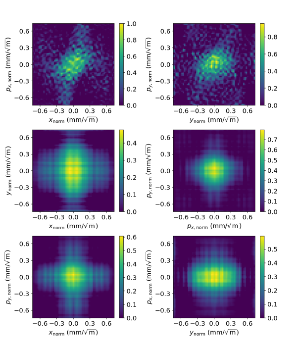
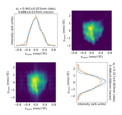
Projections of the reconstructed 4D phase space distribution are shown in Fig. 3 for 10 pC and 100 pC bunch charges. Note that the scales on the axes for each image are given in normalised phase space (units of mm/). Validation images for 10 pC and 100 pC bunch charges are shown in Fig. 4 for three steps in the quadrupole scan. The screen images are generally reproduced from the co-ordinate space projection of the reconstructed phase space distribution with good accuracy, supporting the validity of the reconstructed 4D phase space distribution. The screen images with 100 pC bunch charge show significanly more structure than those with 10 pC bunch charge, though the additional structure is not immediately apparent from the projections of the 4D phase space distribution at the exit of the linac. The richer beam structure observed with 100 pC bunch charge is believed to be associated with the properties of the photoinjector laser.
 |
 |
| (a) 10 pC | (b) 100 pC |
 |
 |
 |
| (a) 10 pC, quadrupole scan step 9. | (b) 10 pC, quadrupole scan step 18. | (c) 10 pC, quadrupole scan step 24. |
 |
 |
 |
| (d) 100 pC, quadrupole scan step 9. | (e) 100 pC, quadrupole scan step 18. | (f) 100 pC, quadrupole scan step 24. |
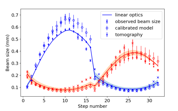
Variations in the beam size at the observation point over the course of a quadrupole scan are shown in Fig. 5. The plots (upper plot for 10 pC bunch charge, and lower plot for 100 pC) compare the beam sizes calculated in four different ways:
-
•
The solid lines (labelled “linear optics”) show the beam sizes (calculated at each point in the quadrupole scan) found by calculating the covariance matrix describing the reconstructed 4D phase space distribution at the reconstruction point, and then transporting the covariance matrix to the observation point. The shaded bands indicate the uncertainties on the beam sizes arising from the uncertainties on the elements of the covariance matrix.
-
•
Crosses (labelled “observed beam size” in Fig. 5) show the rms beam sizes obtained from Gaussian fits to projections of the observed beam images onto the horizontal and vertical axes. The error bars indicate the standard deviations of the rms beam sizes over the ten images collected at each step (which dominate over uncertainties associated with the Gaussian fits).
-
•
The circular markers (labelled “calibrated model”) show the beam sizes at each point in the quadrupole scan expected from the lattice functions in the calibrated model, with emittances found from the reconstructed 4D phase space. The error bars show the uncertainty arising from the uncertainty on the emittance (increased a factor of 10, to make the error bars more clearly visible).
-
•
Points (dots, labelled “tomography”) show the rms beam sizes obtained from Gaussian fits to projections (onto the horizontal and vertical axes) of the reconstructed 4D phase space transported from the reconstruction point to the observation point. The error bars in this case indicate the uncertainties in the fit.
Although there is qualitative agreement between the beam sizes in the calibrated model (using the optics functions shown in Table 1) and the observed beam sizes, there is better agreement with the observed beam sizes in the case of linear transport of the covariance matrix calculated from the reconstructed phase space distribution, and in the case of linear transport of the phase space distribution.


For completeness, and for comparison of the results from tomographic analysis using ART and analysis using machine learning, the emittances and optics functions at the reconstruction point are given in Table 2. The values shown are calculated from the covariance matrices describing the reconstructed 4D phase space distributions, for 10 pC and 100 pC bunch charges. Note that the values given are for the normal mode emittances , and optics functions, , [30]. In terms of these quantities, the covariance matrix is expressed:
| (2) |
where the elements of the covariance matrix are the second-order moments of the beam distribution over all combinations of phase space variables:
| (3) |
with , for , respectively. The symmetric matrices can be written in terms of sub-matrices (with or ):
| (4) |
In the absence of coupling:
| (5) |
and:
| (6) |
| 10 pC | 100 pC | |||
|---|---|---|---|---|
| algebraic reconstruction | machine learning | algebraic reconstruction | machine learning | |
| µm | µm | µm | µm | |
| µm | µm | µm | µm | |
III Phase space tomography using machine learning
Although the results shown in Section II suggest that the algebraic reconstruction technique can be of value in constructing the 4D transverse phase space distribution of the beam in a machine such as CLARA, the method can have some limitations. First, the structures visible in the beam images at the observation point (especially at the higher bunch charge) are not clearly evident in any of the projections shown of the 4D phase space distribution at the reconstruction point. The reasons for this are not well understood: it may simply be a result of the relatively poor resolution with which the 4D phase space distribution is determined; or it may be that the orientation of the distribution in phase space is such as to obscure the structure for the chosen 2D projections — note that the structures seen at the observation point are only really evident for particular steps in the quadrupole scan, i.e. for some specific range of betatron phase advances.
A second limitation of the algebraic reconstruction technique is that it can take some time to process the data to obtain the phase space distribution. The demands in terms of processing time and computational resources increase rapidly with increasing resolution of the reconstruction, and with increasing dimensionality of the phase space. For the results presented here, a phase space resolution of 39 pixels in each dimension of the 4D phase space is used: this limits the detail visible in the phase space, but allows the reconstruction to be completed reasonably rapidly (within a few minutes) using a standard PC. Where a high resolution is required, or a rapid reconstruction would be of value (for example, for several iterations of machine tuning) then more powerful computing resources may be needed if algebraic reconstruction, or a similar tomography technique, is to be used. There is also interest in extending tomography from four to five or six dimensions [16, 12]: this can be of particular value in short-wavelength free electron lasers, for example, where understanding the transverse beam profile and energy spread as a function of longitudinal position in the bunch can be of significant importance.
Approaches based on machine learning may offer ways to address some of the issues associated with conventional tomography techniques for reconstruction of the beam phase space in four (or more) dimensions. The method presented here, which we apply to the two transverse degrees of freedom, uses a pre-trained neural network, to which the beam images at the observation point are provided, in compressed form, as input; the output from the neural network consists of the 4D phase space distribution, again in compressed form. In principle, using a neural network in this way allows a rapid (almost immediate) reconstruction of the 4D phase space distribution once the beam images are provided. The computing resources needed for carrying out the reconstruction can also be much more modest than those needed for algebraic reconstruction tomography. If images in uncompressed form are used, the input and output data sets can still be of significant size, but use of machine learning enables image compression techniques to be applied, reducing the size of input and output data sets. In principle, a neural network can be trained on images and phase space distributions represented in some chosen compressed form, for example as discrete cosine transforms (DCTs) [31, 32, 33]. Image compression would be difficult to apply in the case of conventional tomography methods, which usually rely on a relationship between the sinogram and the object to be reconstructed that is intrinsically expressed in regular co-ordinate space. Neural networks offer much greater flexibility, and do not require a specific representation of the input or output data.
In using a neural network to perform tomographic reconstruction, an issue does arise with the need to train the network. Training must necessarily be based on simulated data, which would ideally include features characteristic of the beam; but at least in cases where the beam shows some detailed structure, the relevant features may not be known at the time of generating the training data. In the current study, we simply take the approach of generating random phase spaces consisting of a number of superposed 4D Gaussian distributions, with the component distributions in each generated phase space varying randomly in position, shape and intensity. Given the shape of the phase space distribution in CLARA suggested by tomography using ART, the phase space distributions constructed in this way may not provide ideal training data; however, it is interesting to consider the ability of a neural network to reconstruct phase space distributions presenting features significantly different from those present in the training data. If the techniques described here are to be of value in a reasonably wide range of situations, then they should be able to reproduce phase space distributions with features significantly different from those in the training data.
III.1 Implementation of machine learning method
Before presenting the results of tomography using machine learning, we discuss some further details of how the technique was implemented.
For preparation of training data, phase space distributions were generated as mentioned above, by superposing 4D Gaussian distributions with random variations in position, shape and intensity. The distributions are constructed in normalised phase space; the sinograms are then obtained by transforming the distribution using phase space rotations (corresponding to the steps in a quadrupole scan), and then projecting the distribution onto the (normalised) – plane at each step in the quadrupole scan. Note that we used phase advances corresponding to those in the calibrated model, shown in Fig. 2 (bottom right). For consistency, it is important that the phase advances should match those resulting from the quadrupole strengths applied in the quadrupole scan, given the lattice functions used for normalising the phase space. It should be emphasised, however, that the chosen lattice functions do not need to match those describing the actual beam distribution (which in general, is not known in advance).
Having obtained the sinograms for the simulated 4D phase space distributions, we compress both the phase space distributions and the sinograms using discrete cosine transforms (DCTs). There are several types of DCT: we use a Type II DCT, which is the default in many standard scientific computing packages. In the case of a 2D array, a Type II DCT is defined by:
| (7) |
where the values are the components of the initial array, and (for , ) are the components of the transformed array. Compression is achieved by truncating the transformed array at some point, either defined in terms of the magnitudes of the components (which should all be below some specified threshold beyond the truncation point) or simply in terms of a fixed limit on the size of the transformed array. The inverse of the Type II DCT of an array is given by:
| (8) |
where:
| (9) |
The expressions in (7) and (8) can be extended to higher-dimensional arrays by including an additional summation for each additional index, and making the appropriate modification to the numerical factors in (8). Truncating the transformed array corresponds to reducing the upper limits on the summations in the inverse transformation (8); in this case, the array is reconstructed with approximated values for its elements, but the number of elements in the array remains the same. In the case of an image, the effect of truncating the DCT is to lose some of the fine detail. Figure 6 illustrates image compression using DCTs truncated to different sizes, using (as an example) a beam image collected during the quadrupole scan with 100 pC bunch charge. The original image has resolution (in pixels) . Truncating the DCT to results in some loss of clarity, but the main features and some details can still be clearly seen. Truncation to results in more significant loss of detail.

The training data for the neural network consists of some number of pairs of the DCTs of the sinograms (input) and corresponding phase space distributions (output). The neural network itself is implemented in Keras [34]. We use a rather straightforward architecture. Apart from the input and output layers, there are two hidden layers, defined as dense layers in Keras. To limit overtraining, each dense layer is followed by a dropout layer. We use a resolution of 19 points on each axis for the DCT of the 4D phase space (i.e. voxels in total), and a resolution of for the DCT of each 2D projection in the set of “images” forming the sinogram. In practice, these resolutions capture sufficient numbers of DCT modes to allow representation of the screen images and the 4D phase space with good resolution. Note that the size of the data for the 4D phase space using machine learning () is substantially smaller than the size used for the ART tomography reported in Section II (). We have found that for the data collected in CLARA, increasing the numbers of DCT modes, either in the input sinograms or the reconstructed phase space, does not improve the quality of the results as judged by a comparison between the projections of the phase space at the observation point, and the original beam images (as shown, for example, in Fig. 11). In constructing the sinogram, we use phase space rotations corresponding to the phase advances in the calibrated model (see Fig. 2, bottom right plot), i.e. with 32 steps in the quadrupole scan. With these parameters, the neural network has an input layer with nodes, and an output layer with nodes. We use 1500 and 3000 nodes for the first and second hidden (dense) layers, respectively, with a dropout layer specified to set 20% of inputs (selected randomly) to zero for each dense layer during training. The tomography process using image compression and machine learning is illustrated schematically in Fig. 7.

A total of 3000 sets of 4D phase space distributions and sinograms were generated as training data; 100 sets were reserved as validation sets for testing the performance of the trained network, and were not used in the training process itself. Training was carried out using the Adam optimization algorithm [35]. Training takes several minutes on a standard laptop PC. The training time is comparable to the time taken to process a single data set using ART; however, training only needs to be performed once, to produce a neural network that can (in principle) be applied to any data set collected in a quadrupole scan using given quadrupole strengths. The ART analysis would need to be performed separately for each data set.
Two examples illustrating results from the trained network are shown in Fig. 8. The examples are selected at random from the validation data sets. Each row of images in the figure shows a different projection of a 4D phase space: in each example, the top row shows the projections from the original phase space, and the bottom row shows the projections from the phase space reconstructed by the neural network when provided with the (DCTs of the) corresponding sinograms. While there are clearly some differences between the original and the reconstructed phase spaces, the reconstruction is sufficiently similar to the original to provide a useful practical indication of the beam distribution in phase space.

Example 1

Example 2
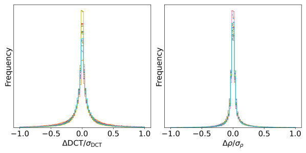
To characterise further the reliability of the machine learning reconstruction of the phase space, we calculate the residuals between the original phase space density in the test data and the phase space density found from the sinograms using the trained neural network. The residuals are shown in Fig. 9, as histograms of and . Here, is the difference between a particular DCT coefficient predicted by the neural network, and the corresponding DCT coefficient in the phase space distribution used to generate the sinogram data provided as input to the network. is the standard deviation of the DCT coefficients. is the difference in the phase space density (at a particular element of 4D phase space) between the original distribution and the distribution found by the neural network, after performing an inverse DCT of the network output; and is the standard deviation of the phase space density. Figure 9 shows histograms of these quantities for 20 cases from the validation data sets. Typically, between 75% and 80% of phase space density values from the neural network are within 0.1 of the true phase space density.
III.2 Experimental results from tomography using machine learning
The trained neural network was applied to analysis of the quadrupole scan data collected on CLARA, described in Section II. The screen images from each step of the quadrupole scan were prepared in the same way as for the ART analysis, by cropping, and then scaling to transform to normalised phase space. The images were then compressed by constructing the DCTs, which were truncated to 21 modes on each axis. The DCTs were provided as input to the trained neural network, which provided the DCT of the 4D phase space distribution, with resolution 19 modes along each axis. Projections from the reconstructed 4D phase space distribution for 10 pC and 100 pC bunch charges are shown in Fig. 10.
 |
 |
| (a) 10 pC | (b) 100 pC |
In Section II, we validated the ART reconstruction of the 4D phase space distribution by comparing the projection of the distribution onto – co-ordinate space at the observation point with the observed beam images at different steps of the quadrupole scan. We can make similar comparisons to validate the 4D phase space distribution reconstructed using the neural network: some examples (for the same steps as shown in Fig. 4) are shown in Fig. 11. Once again, we see generally good agreement between the projection of the 4D phase space distribution and the observed images, in both the 10 pC and the 100 pC cases. Comparing with projections from the phase space reconstructed using ART in Fig. 4, the machine learning projections do not all have the same clarity, in terms of the finer details in some of the images. It should be remembered, however, that the ART tomography uses beam images with resolution 3939 pixels, to reconstruct the 4D phase space distribution with a resolution of 39 pixels on each axis. The machine learning technique uses beam images and 4D phase space in a compressed form: the beam images are represented by 21 DCT modes on each axis, and the phase space is represented by 19 DCT modes on each axis. Although this is sufficient to capture a significant amount of detail, the truncation of the DCTs means that the compression is not lossless. Given the compression ratio, the machine learning method retains a reasonable level of detail in the phase space distribution.
Comparisons between the observed and reconstructed beam sizes are shown in Fig. 12: the results here can be compared with those in Fig. 5, which shows the beam sizes reconstructed using ART. While there are some differences in detail in the quality of the match between the beam sizes expected from the reconstructed phase space and the beam sizes observed during the quadrupole scan, both the ART and the machine learning techniques show similar performance in describing the beam behaviour.
 |
 |
 |
| (a) 10 pC, quadrupole scan step 9. | (b) 10 pC, quadrupole scan step 18. | (c) 10 pC, quadrupole scan step 24. |
 |
 |
 |
| (d) 100 pC, quadrupole scan step 9. | (e) 100 pC, quadrupole scan step 18. | (f) 100 pC, quadrupole scan step 24. |

IV Conclusions and possible further developments
The machine learning technique we have described in this paper uses relatively simple methods for reconstructing the 4D phase space. Nevertheless, this approach appears capable of producing useful results, as shown by the comparison between projections onto – co-ordinate space at the observation point for different quadrupole strengths, and beam images collected over the course of a quadrupole scan. Values obtained for parameters describing the distribution (emittances and lattice functions) are consistent with those obtained using a conventional tomography technique. Data collection and analysis were planned using a design model of the machine; despite significant differences between the design model and the actual machine conditions during collection of experimental data, results from both the ART and the machine learning techniques provide useful information on the beam properties in CLARA.
Use of image compression (in the present case, using discrete cosine transforms) allows reduction of the size of the data sets that need to be processed, in particular, for representing the 4D phase space. Machine learning allows direct tomographic analysis of compressed beam images and phase space representations, without the additional complications or difficulties that would be encountered in attempting to apply conventional tomography techniques to compressed images.
Inspection of projections of the 4D phase space onto various planes (in particular, comparison of Fig. 3 with Fig. 10) suggests that the machine learning technique is capable of producing a representation of the 4D phase space distribution that appears clearer than that obtained by the conventional tomography algorithm. On the other hand, the beam images obtained by projecting the 4D phase space distribution onto co-ordinate space at the observation point have slightly higher fidelity in the case of the conventional tomography technique. Nevertheless, the consistency in the results of the two methods, and the fact that the neural network produces a 4D phase space distribution immediately the quadrupole scan images are available (compared to a potentially lengthy computation time required by the conventional tomography technique) suggests that the machine learning approach could have some practical value.
There are a number of ways in which the machine learning approach could be further developed. With an improved understanding of the operational conditions of CLARA, some optimisation would be possible in terms of the quadrupole strengths (and number of steps) used in the quadrupole scan. More sophisticated neural network architectures, or use of more sophisticated machine learning tools generally, could lead to a better reconstruction of the 4D phase space distribution from a given set of sinograms. There may be some benefits in further increasing the number of sets of training data. An indication of the quality to be expected in the reconstruction can be obtained using simulated data, for example by calculating the residuals as shown in Fig. 9. Although the phase space distributions in the training data we used for the neural network had very different features from the phase space distribution in the real machine, the trained network was still capable of reconstructing a phase space distribution that provided a good description of beam behaviour. It is possible, however, that using training data more closely resembling the real beam (once some initial characterisation of the beam has been obtained) could lead to better results.
Discrete cosine transforms may not be the optimal way to represent images and phase space distributions in compressed form for the application described here. A DCT essentially represents a multidimensional array as a set of orthogonal modes, with each mode described by a cosine function. This provides a convenient general purpose approach, but alternative basis functions may allow more accurate representation of beam images and phase space distributions with fewer modes. It may be possible, for example, to take advantage of properties generally expected of the beam (such as approximate symmetries) to construct a more appropriate basis. The scope for further development is rather wide, and while the results shown here are encouraging and demonstrate the value of machine learning for tomographic reconstruction in principle, more extensive studies would be required to understand the full potential of the technique.
Acknowledgements.
We would like to thank our colleagues in STFC/ASTeC at Daresbury Laboratory for help and support with various aspects of the simulation and experimental studies of CLARA. In particular, we would like to thank Amy Pollard for useful discussions and advice on machine learning. This work was supported by the Science and Technology Facilities Council, UK, through a grant to the Cockcroft Institute.References
- [1] C.B. McKee, P.G. O’Shea, J.M.J. Madey, “Phase space tomography of relativistic electron beams”, Nucl. Instrum. Methods Phys. Res., Sect. A , 264–267 (1995).
- [2] V. Yakimenko, M. Babzien, I. Ben-Zvi, R. Malone and X.-J. Wang, “Electron beam phase-space measurement using a high-precision tomography technique”, Phys. Rev. ST Accel. Beams , 112801 (2006).
- [3] D. Stratakis, R.A. Kishek, H. Li, S. Bernal, M. Walter, B. Quinn, M. Reiser and P.G. O’Shea, “Tomography as a diagnostic tool for phase space mapping of intense particle beams”, Phys. Rev. ST Accel. Beams , 122801 (2003).
- [4] D. Stratakis, K. Tian, R.A. Kishek, I. Haber, M. Reiser and P.G. O’Shea, “Tomographic phase-space mapping of intense particle beams using solenoids”, Physics of Plasmas , 120703 (2007).
- [5] Dao Xiang, Ying-Chao Du, Li-Xin Yan, Ren-Kai Li, Wen-Hui Huang, Chuan-Xiang Tang, and Yu-Zheng Lin, “Transverse phase space tomography using a solenoid applied to a thermal emittance measurement”, Phys. Rev. ST Accel. Beams , 022801 (2009).
- [6] Michael Röhrs, Christopher Gerth, Holger Schlarb, Bernhard Schmidt, and Peter Schmüser, “Time-resolved electron beam phase space tomography at a soft x-ray free-electron laser”, Phys. Rev. ST Accel. Beams , 050704 (2009).
- [7] Q.Z. Xing, L. Du, X.L. Guan, C.X. Tang, M.W. Wang, X.W. Wang and S.X. Zheng, “Transverse profile tomography of a high current proton beam with a multi-wire scanner”, Phys. Rev. Accel. Beams , 072801 (2018).
- [8] Fuhao Ji, Jorge Giner Navarro, Pietro Musumeci, Daniel B. Durham, Andrew M. Minor and Daniele Filippetto, “Knife-edge based measurement of the 4D transverse phase space of electron beams with picometer-scale emittance”, Phys. Rev. Accel. Beams , 082801 (2019).
- [9] D. Alesinia, G. Di Pirro, L. Ficcadenti, A. Mostacci, L. Palumbo, J. Rosenzweig and C. Vaccarezza, “RF deflector design and measurements for the longitudinal and transverse phase space characterization at SPARC”, Nucl. Instrum. Methods Phys. Res., Sect. A , 488–502 (2006).
- [10] D. Marx, R.W. Assmann, P. Craievich, K. Floettmann, A. Grudiev and B. Marchetti, “Simulation studies for characterizing ultrashort bunches using novel polarizable X-band transverse defection structures”, Scientific Reports, 9:19912 (2019).
- [11] S. Jaster-Merz, R.W. Assmann, R. Brinkmann, F. Burkart, T. Vinatier, “5D tomography of electron bunches at ARES”, in Proceedings of the 13th International Particle Accelerator Conference, Bangkok, Thailand, 2022, pp. 279–283.
- [12] A. Scheinker, D. Filippetto and F. Cropp, “6D phase space diagnostics based on adaptively tuned physics-informed generative convolutional neural networks”, in Proceedings of the 13th International Particle Accelerator Conference, Bangkok, Thailand, 2022, pp. 776–779.
- [13] G. Wang, J.C. Ye and B. De Man, “Deep learning for tomographic image reconstruction”, Nature Machine Intelligence , 737–748 (2020).
- [14] Y. Li, W. Cheng, L.H. Yu and R. Rainer, “Genetic algorithm enhanced by machine learning in dynamic aperture optimization”, Phys. Rev. Accel. Beams , 054601 (2018).
- [15] J. Wan, P. Chu, Y. Jiao, Y. Li, “Improvement of machine learning enhanced genetic algorithm for nonlinear beam dynamics optimization”, Nucl. Instrum. Methods Phys. Res., Sect. A , 162683 (2019).
- [16] A. Edelen, N. Neveu, M. Frey, Y. Huber, C. Mayes and A. Adelmann, “Machine learning for orders of magnitude speedup in multiobjective optimization of particle accelerator systems”, Phys. Rev. Accel. Beams , 044601 (2020).
- [17] C. Emma, A. Edelen, M.J. Hogan, B. O’Shea, G. White, and V. Yakimenko, “Machine learning-based longitudinal phase space prediction of particle accelerators”, Phys. Rev. Accel. Beams , 112802 (2018).
- [18] G. Azzopardi, G. Valentino, A. Muscat, B. Salvachua, “Automatic spike detection in beam loss signals for LHC collimator alignment”, Nucl. Instrum. Methods Phys. Res., Sect. A , 10–18 (2019).
- [19] X. Xu, Y. Zhou and Y. Leng, “Machine learning based image processing technology application in bunch longitudinal phase information extraction”, Phys. Rev. Accel. Beams , 032805 (2020).
- [20] C. Tennant, A. Carpenter, T. Powers, A.S. Solopova and L. Vidyaratne, “Superconducting radio-frequency cavity fault classification using machine learning at Jefferson Laboratory”, Phys. Rev. Accel. Beams , 114601 (2020).
- [21] Z. Omarov, S. Haciömeroğlu, “Machine learning assisted non-destructive beam profile monitoring”, Nucl. Instrum. Methods Phys. Res., Sect. A , 166132 (2022).
- [22] L. Emery, H. Shang, Y. Sun and X. Huang, “Application of a machine learning based algorithm to online optimization of the nonlinear beam dynamics of the Argonne Advanced Photon Source”, Phys. Rev. Accel. Beams , 082802 (2021).
- [23] P. Arpaia, G. Azzopardi, F. Blanc et al., “Machine learning for beam dynamics studies at the CERN Large Hadron Collider”, Nucl. Instrum. Methods Phys. Res., Sect. A , 164652 (2021).
- [24] J.A. Clarke, D. Angal-Kalinin, N. Bliss, R. Buckley, S. Buckley, R. Cash, P. Corlett, L. Cowie, G. Cox, G.P. Diakun, D.J. Dunning, B.D. Fell, A. Gallagher, P. Goudket, A.R. Goulden, D.M.P. Holland, S.P. Jamison, J.K. Jones, A.S. Kalinin, W. Liggins, L. Ma, K.B. Marinov, B. Martlew, P.A. McIntosh, J.W. McKenzie, K.J. Middleman, B.L. Militsyn, A.J. Moss, B.D. Muratori, M.D. Roper, R. Santer, Y. Saveliev, E. Snedden, R.J. Smith, S.L. Smith, M. Surman, T. Thakker, N.R. Thompson, R. Valizadeh, A.E. Wheelhouse, P.H. Williams, R. Bartolini, I. Martin, R. Barlow, A. Kolano, G. Burt, S. Chattopadhyay, D. Newton, A. Wolski, R.B. Appleby, H.L. Owen, M. Serluca, G. Xia, S. Boogert, A. Lyapin, L. Campbell, B.W.J. McNeil, and V.V. Paramonov CLARA Conceptual Design Report, (STFC, Daresbury, Warrington, UK, 2013).
- [25] D. Angal-Kalinin, A.D. Brynes, R.K. Buckley, S.R. Buckley, R.J. Cash, H.M. Castaneda Cortes, J.A. Clarke, R.F. Clarke, P.A. Corlett, L.S. Cowie, G. Cox, K.D. Dumbell, D.J. Dunning, B.D. Fell, P. Goudket, A.R. Goulden, S.A. Griffiths, M.D. Hancock, J. Henderson, J.P. Hindley, C. Hodgkinson, F. Jackson, J.K. Jones, N.Y. Joshi, S.L. Mathisen, J.W. McKenzie, K.J. Middleman, B.L. Militsyn, A.J. Moss, B.D. Muratori, T.C.Q. Noakes, A. Oates, T.H. Pacey, M.D. Roper, Y.M. Saveliev, D.J. Scott, B.J.A. Shepherd, R.J. Smith, W. Smith, E.W. Snedden, M. Surman, N. Thompson, C. Tollervey, R. Valizadeh, D.A. Walsh, T.M. Weston, A.E. Wheelhouse, P.H. Williams, and J.T.G. Wilson, “Status of CLARA Front End commissioning and first user experiments”, in Proceedings of the 10th International Particle Accelerator Conference, Melbourne, Australia, 2019, pp. 1851–1854.
- [26] D. Angal-Kalinin et al, “Design, specifications, and first beam measurements of the compact linear accelerator for resarch and applications front end”, Phys. Rev. Accel. Beams , 044801 (2020).
- [27] A. Wolski, D.C. Christie, B.L. Militsyn, D.J. Scott, H. Kockelbergh, “Transverse phase space characterization in an accelerator test facility”, Phys. Rev. Accel. Beams , 032804 (2020).
- [28] D.J. Scott, A.D. Brynes, M.P. King, “High level software development framework and activities on VELA/CLARA”, in Proceedings of the 10th International Particle Accelerator Conference, Melbourne, Australia, 2019, pp. 1855–1858.
- [29] K.M. Hock, M.G. Ibison, D.J. Holder, A. Wolski and B.D. Muratori, “Beam tomography in transverse normalised phase space”, Nucl. Instrum. Methods Phys. Res., Sect. A , 36–44 (2011).
- [30] A. Wolski, “Alternative approach to general coupled linear optics,” Phys. Rev. ST Accel. Beams , 024001 (2006).
- [31] N. Ahmed, T. Natarajan, K.R. Rao, “Discrete cosine transform”, in IEEE Transactions on Computers, C-23, 1, 90–93 (1974).
- [32] Wen-Hsiung Chen and W. Pratt, “Scene Adaptive Coder”, in IEEE Transactions on Communications, 32, 3, 225–232 (1984).
- [33] K.R. Rao and P. Yip, “Discrete cosine transform: algorithms, advantages, applications”, Academic Press, San Diego, CA, USA (1990). ISBN:978-0-08-092534-9
- [34] Keras documentation, https://keras.io (retrieved 11 August 2022).
- [35] D.P. Kingma and J. Ba, “Adam: a method for stochastic optimization,” arXiv:1412.6980v9 (2017).