Transport in honeycomb lattice with random $\pi$-fluxes: Implications for low-temperature thermal transport in the Kitaev spin liquids

Quantum spin liquids (QSLs) are an exotic state of matter with no local symmetry breaking, deconfined fractionalized quasiparticles, and emergent gauge excitations [1, 2, 3]. The Kitaev model, an exactly solvable honeycomb model, provides a typical framework for describing such a phase, where spins fractionalize to Majorana fermions and $Z_{2}$ gauge excitations (visons) [4]. Thanks to the proposal by Jackeli and Khaliullin [5], which suggests that the Kitaev model can be realized in certain strongly spin-orbit coupled systems, a growing number of Kitaev candidate materials have been discovered in the past decade [6, 7].

Despite the theoretical proposal of QSLs for several decades, their experimental identification remains challenging. Thermal transport experiments are a promising technique for characterizing QSLs, as they allow the detection of charge-neutral, mobile quasiparticles. For example, in the Kitaev candidate material $\alpha-\text{RuCl}_{3}$, a half-quantized thermal Hall conductance has been observed, indicating the existence of a chiral Majorana mode at the edge of the non-Abelian Kitaev spin liquid [8, 9, 10]. To fully understand the experimental results, it is crucial to predict the thermal transport signatures of QSLs, particularly those proximate to the exact Kitaev model, in various different regimes [11, 12, 13, 14, 15, 16, 17, 18, 19, 20, 21].

The longitudinal thermal conductivity $\kappa_{\text{xx}}(\omega,T)$ of the Kitaev model has been numerically investigated using Kubo’s formalism, and the DC thermal conductivity $\kappa_{\text{K}}(T)$ can be obtained by extrapolation of $\kappa_{\text{xx}}(\omega,T)$ to the $\omega\rightarrow 0$ limit [11, 12, 13, 14, 15]. When the temperature $T$ is comparable to or smaller than the vison gap $\Delta_{v}$, such extrapolation appears to give results with significant error bars and calculations with larger system sizes are needed [11, 15], leaving the low-temperature behavior of $\kappa_{\text{K}}$ inconclusive. Neglecting the gauge excitations in the Kitaev model, it is possible to regard an undoped graphene as two stacks of the Kitaev model, and thus expect that the thermal transport of Kitaev spin liquid and the electric transport of graphene may have similar low-temperature behavior. It was proposed that in graphene there exists a universal minimum electrical conductivity $\sigma_{\text{min}}=e^{2}/\pi h$ per valley per spin, regardless of the concentration of disorders [22, 23, 24]. It is thus natural to ask whether a similar ‘minimum thermal conductivity’ (MTC) also exists in a pure Kitaev model. A previous quantum Monte Carlo study seems to support the existence of MTC in the low-temperature regime, i.e. $\lim_{T\rightarrow 0}\kappa_{\text{K}}/T=k_{B}^{2}/12\hbar$, but further justification is required due to the significant uncertainties and finite-size effects in the numerical simulation [11]. Moreover, at low temperatures, the phase coherence length may exceed the dimensions of a realistic sample, within which the quantum interference effects are essential. Consequently, the thermally excited random $Z_{2}$ flux background may strongly localize Majorana particles [25, 14, 26], provided that the localization length is smaller than the system size. Such localization effects are uncaptured by previous calculations performed for relatively small systems, and overlooking these effects may crucially affect the interpretation of experimental results.

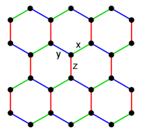
To understand the low-temperature thermal conductivity of the Kitaev model in the absence of disorder and magnetic fields, in this work we numerically study the transport of complex fermions in a random $\pi$-flux honeycomb model (RPFHM) near half-filling. This approach is motivated by the observation that the Kitaev model (see Fig. 1) can be seen as half of the RPFHM (see Fig. 1), and the thermal conductivity of the former is linked to the electrical conductivity of the latter via the Wiedemann-Franz (WF) law. Furthermore, the RPFHM is of academic interest on its own, as this random $Z_{2}$-flux problem is less studied compared to random $U(1)$-flux models [27, 28, 29, 30, 31].

We focus on the zero-temperature longitudinal DC conductivity of the RPFHM and its localization properties as a function of flux density and chemical potential. We extract the dependence of DC conductivity on flux density and Fermi wavevector in the semi-classical diffusive regime. Our analysis reveals Anderson localization due to random $\pi$-fluxes, and we obtain 2-D localization lengths. Our results indicate that the low-temperature thermal conductivity of a clean Kitaev model neither exhibits MTC nor vanishes, but instead diverges as $\kappa_{\text{K}}\sim T^{3}e^{\Delta_{v}/k_{B}T}$, which is unexpected based on previous studies. Additionally, when $k_{B}T\sim\Delta_{v}$, the thermal conductivity could be significantly suppressed due to strong Majorana localization.

The low-temperature behavior of thermal conductivity $\kappa_{\text{K}}$ of the Kitaev model can be inferred using earlier results. We first briefly introduce the Kitaev model [4]

where Pauli matrices $\vec{\sigma_{i}}=(\sigma^{x}_{i},\sigma^{y}_{i},\sigma^{z}_{i})$ describe the spin degrees of freedom on site $i$, $\langle ij\rangle_{\lambda}$ denotes the $\lambda$-type nearest-neighbor bond ($\lambda=x,y,z$) between site $i$ and $j$ and each bond is only summed once, as shown in Fig. 1. In this work, we are only interested in the isotropic case so we set $J=J_{x}=J_{y}=J_{z}$ hereafter. The Kitaev model can be exactly solved by mapping spins to Majorana fermions and the Hamiltonian becomes

where the Majorana fermions satisfy anticommutation relations $\{\gamma_{i},\gamma_{j}\}=2\delta_{ij}$, and the bond operator $\tilde{u}_{ij}=-\tilde{u}_{ji}=\pm 1$ acts as a $Z_{2}$ gauge field.

After making a gauge transformation $f_{j}^{\dagger}\rightarrow-if_{j}^{\dagger},j\in A$ sublattice, followed by a Majorana transformation $f_{i}^{\dagger}=(\gamma_{i}^{1}+i\gamma_{i}^{2})/2$ to Eq. (1), one can see the RPFHM (1) is exactly two copies of the Kitaev model (10), with $t=2J$. Therefore the thermal conductivity of the Kitaev model (9) is half of that of the RPFHM (1), namely $\kappa_{\text{G}}=2\kappa_{\text{K}}$, provided both have the same flux configuration. At thermal equilibrium, $\kappa_{\text{K}}$ can be expressed as the weighted average of thermal conductivity $\kappa_{\text{K}}^{\vbox{\hbox{\scalebox{0.7}{$\varhexagon$}}}}$ over every flux configuration $\varhexagon$, namely $\kappa_{\text{K}}=(\sum_{\vbox{\hbox{\scalebox{0.7}{$\varhexagon$}}}}Z_{\vbox{\hbox{\scalebox{0.7}{$\varhexagon$}}}}\kappa_{\text{K}}^{\vbox{\hbox{\scalebox{0.7}{$\varhexagon$}}}})/(\sum_{\vbox{\hbox{\scalebox{0.7}{$\varhexagon$}}}}Z_{\vbox{\hbox{\scalebox{0.7}{$\varhexagon$}}}})$. Here $Z_{\vbox{\hbox{\scalebox{0.7}{$\varhexagon$}}}}=\text{Tr}e^{-\beta H_{\vbox{\hbox{\scalebox{0.7}{$\varhexagon$}}}}}$ is the partition function for specific flux configuration $\varhexagon$ described by the Hamiltonian $H_{\vbox{\hbox{\scalebox{0.7}{$\varhexagon$}}}}$, and $\sum_{\vbox{\hbox{\scalebox{0.7}{$\varhexagon$}}}}$ denotes sum over all flux configurations. In the Kitaev model the ground state contains no flux [62], while at temperatures much lower than the vison gap $\Delta_{v}\approx 0.1536J$ [4], thermally excited visons are dilute and may be regarded as uncorrelated on different plaquettes, with flux density approximately given by

Here we emphasize that although the calculation of $\kappa_{\text{K}}$ seems a quenched disorder problem, it is an artifact as the bond variables $u_{ij}$ commute with the Hamiltonian. In fact, it is still an annealed average problem, as the free energy is given by $\mathcal{F}=-k_{B}T\ln\sum_{\vbox{\hbox{\scalebox{0.7}{$\varhexagon$}}}}Z_{\vbox{\hbox{\scalebox{0.7}{$\varhexagon$}}}}$, where the logarithm is taken after the sum over all flux configurations is computed.

The thermal conductivity $\kappa_{\text{G}}$ of RPFHM is linked to the electrical conductivity $\sigma_{G}$ by the Wiedemann–Franz (WF) law $\kappa_{\text{G}}=\sigma_{\text{G}}\mathcal{L}T$ where $\mathcal{L}$ is the Lorentz number. For a non-interacting Fermi liquid, the Lorentz number is a universal constant $\mathcal{L}_{0}=\pi^{2}k_{B}^{2}/3e^{2}$, while around the Dirac point, the Lorentz number may be a few times larger than $\mathcal{L}_{0}$ even for the non-interacting case [63, 64]. Combining the above arguments, one obtains

where $\sigma_{\text{G}}(n_{v},T,\mu)$ denotes the DC conductivity of RPFHM, which has flux density $n_{v}$, Fermi level $\mu$ and temperature $T$.

We shall now demonstrate the low-temperature behavior of $\kappa_{\text{K}}$ using Eq. (12). As $k_{B}T\gg|\mu|$, the conduction is mainly contributed by the thermally excited quasiparticles with energy $E\sim k_{B}T$. When $k_{B}T\ll\Delta_{v}$, we observe that the thermal de Broglie wavelength $\lambda_{\text{th}}\sim T^{-1}$ is much shorter than the mean flux distance $r_{m}\sim e^{\Delta_{v}/2k_{B}T}$. This indicates that the transport is away from the Dirac point and in the semiclassical regime. As the localization length is exponentially large $\xi\approx l_{0}e^{\pi k_{F}l_{e}}$ in this regime, the localization effects are negligible for realistic system size, or when the phase coherence length is much smaller than the localization length $L_{\phi}\ll\xi$ due to the coupling to environments. Substituting the thermal de Broglie wavevector $k_{\text{th}}=2\pi/\lambda_{\text{th}}$ to Eq. (4) (see appendix A for the justification), which is applicable when $k_{\text{th}}r_{m}\gg 1$, and using Eqs. (11)(12), one obtains diverging thermal conductivity $\kappa_{\text{K}}\sim T^{3}e^{\Delta_{v}/k_{B}T}$ at low temperatures. When $k_{B}T\sim\Delta_{v}\approx 0.15J$, which corresponds to $\lambda_{\text{th}}\gtrsim r_{m}$, the thermal transport is in the quantum regime and localization effects are non-negligible. We assume both the system size $L$ and phase coherence length $L_{\phi}$ is much larger than the thermal localization length $\xi_{T}=\xi(n_{v}(T),k_{\text{th}}(T))$, which is estimated to be a few hundred of lattice spacing from Fig. 5. In this case, the Majorana fermions are strongly localized and significantly suppressed thermal conductivity $\kappa_{\text{K}}/T\ll k_{B}^{2}/2\pi\hbar$ may be observable. This is in contrast with the low-temperature case $k_{B}T\ll\Delta_{v}$ where $\kappa_{\text{K}}/T\gg k_{B}^{2}/2\pi\hbar$ and analogous to the large resistivity $\rho\gg h/e^{2}$ observed in graphene due to the strong localization [65, 66, 67]. We note that it is difficult to obtain $\kappa_{\text{K}}$ at higher temperature $k_{B}T\sim J\gg\Delta_{v}$ using our calculations, as the thermal transport is also contributed by quasiparticles at high energies that are not considered in this work. Besides, in this regime visons can no longer be regarded as dilute, and the validity of Eq. (11) becomes questionable.

In this work, we have utilized a combination of numerical methods to investigate the transport of RPFHM near the Dirac point. Our results reveal that when the wavelength of Dirac fermion is much shorter than the average flux spacing, the semiclassical DC conductivity is quadratic in the Fermi momentum and inversely proportional to the flux density. We have also demonstrated that intervalley scattering by the $\pi$-fluxes leads to weak (strong) localization of Dirac fermions at high (low) Fermi energy.

Our results imply that the thermal transport of the Kitaev model is semiclassical at low temperatures $k_{B}T\ll\Delta_{v}$, and that the thermal conductivity diverges as $\kappa_{\text{K}}\sim T^{3}e^{\Delta_{v}/k_{B}T}$. When $k_{B}T\sim\Delta_{v}$, the itinerant Majorana fermions may be strongly localized, leading to a significantly suppressed thermal conductivity $\kappa_{\text{K}}/T\ll k_{B}^{2}/2\pi\hbar$. Our predictions are expected to hold even in the presence of disorder as long as $\tau_{v}^{-1}\gg\tau_{d}^{-1}$, where $\tau_{v}^{-1}(\tau_{d}^{-1})$ is the scattering rate due to vison (disorder). When the temperature is much smaller than the crossover temperature $T_{d}$ at which $\tau_{d}^{-1}=\tau_{v}^{-1}$, the disorder becomes the dominant source of elastic scattering and the transport is similar to that of an undoped graphene. Consequently, $\kappa_{\text{K}}/T$ should reduce with decreasing temperature and finally saturates to a value comparable or smaller to $1/2\pi\hbar$ [35, 52, 53]. Such temperature dependence, as shown in Fig. 6, was unseen in previous numerical simulations and may be observable in a clean sample at very low temperatures. In realistic Kitaev materials, non-Kitaev-type interactions also allow the hopping of visons and may have important consequences [16, 18], which are left for future studies.

References

- Anderson [1973] P. W. Anderson, Resonating valence bonds: A new kind of insulator?, Materials Research Bulletin 8, 153 (1973).
- Savary and Balents [2016] L. Savary and L. Balents, Quantum spin liquids: a review, Reports on Progress in Physics 80, 016502 (2016).
- Zhou et al. [2017] Y. Zhou, K. Kanoda, and T.-K. Ng, Quantum spin liquid states, Rev. Mod. Phys. 89, 025003 (2017).
- lieb [2006] A. lieb, Anyons in an exactly solved model and beyond, Annals of Physics 321, 2 (2006).
- Jackeli and Khaliullin [2009] G. Jackeli and G. Khaliullin, Mott insulators in the strong spin-orbit coupling limit: From Heisenberg to a quantum compass and Kitaev models, Phys. Rev. Lett. 102, 017205 (2009).
- Winter et al. [2017] S. M. Winter, A. A. Tsirlin, M. Daghofer, J. van den Brink, Y. Singh, P. Gegenwart, and R. Valentí, Models and materials for generalized kitaev magnetism, Journal of Physics: Condensed Matter 29, 493002 (2017).
- Trebst and Hickey [2022] S. Trebst and C. Hickey, Kitaev materials, Physics Reports 950, 1 (2022).
- Kasahara et al. [2018a] Y. Kasahara, K. Sugii, T. Ohnishi, M. Shimozawa, M. Yamashita, N. Kurita, H. Tanaka, J. Nasu, Y. Motome, T. Shibauchi, and Y. Matsuda, Unusual thermal hall effect in a Kitaev spin liquid candidate , Phys. Rev. Lett. 120, 217205 (2018a).
- Kasahara et al. [2018b] Y. Kasahara, T. Ohnishi, Y. Mizukami, O. Tanaka, S. Ma, K. Sugii, N. Kurita, H. Tanaka, J. Nasu, Y. Motome, et al., Majorana quantization and half-integer thermal quantum Hall effect in a Kitaev spin liquid, Nature 559, 227 (2018b).
- Yokoi et al. [2021] T. Yokoi, S. Ma, Y. Kasahara, S. Kasahara, T. Shibauchi, N. Kurita, H. Tanaka, J. Nasu, Y. Motome, C. Hickey, S. Trebst, and Y. Matsuda, Half-integer quantized anomalous thermal Hall effect in the Kitaev material candidate -RuCl3, Science 373, 568 (2021).
- Nasu et al. [2017] J. Nasu, J. Yoshitake, and Y. Motome, Thermal transport in the Kitaev model, Phys. Rev. Lett. 119, 127204 (2017).
- Metavitsiadis et al. [2017] A. Metavitsiadis, A. Pidatella, and W. Brenig, Thermal transport in a two-dimensional spin liquid, Phys. Rev. B 96, 205121 (2017).
- Pidatella et al. [2019] A. Pidatella, A. Metavitsiadis, and W. Brenig, Heat transport in the anisotropic kitaev spin liquid, Phys. Rev. B 99, 075141 (2019).
- Kao and Perkins [2021] W.-H. Kao and N. B. Perkins, Disorder upon disorder: Localization effects in the Kitaev spin liquid, Annals of Physics 435, 168506 (2021), special issue on Philip W. Anderson.
- Nasu and Motome [2020] J. Nasu and Y. Motome, Thermodynamic and transport properties in disordered Kitaev models, Phys. Rev. B 102, 054437 (2020).
- Joy and Rosch [2022] A. P. Joy and A. Rosch, Dynamics of Visons and Thermal Hall Effect in Perturbed Kitaev Models, Phys. Rev. X 12, 041004 (2022).
- Zheng and Brataas [2021] J.-H. Zheng and A. Brataas, Controlling the RKKY interaction and heat transport in a Kitaev spin liquid via flux walls, Phys. Rev. B 104, 064437 (2021).
- Chen and Villadiego [2023] C. Chen and I. S. Villadiego, Nature of visons in the perturbed ferromagnetic and antiferromagnetic kitaev honeycomb models, Phys. Rev. B 107, 045114 (2023).
- Koyama and Nasu [2021] S. Koyama and J. Nasu, Field-angle dependence of thermal hall conductivity in a magnetically ordered kitaev-heisenberg system, Phys. Rev. B 104, 075121 (2021).
- Zhang et al. [2021] E. Z. Zhang, L. E. Chern, and Y. B. Kim, Topological magnons for thermal hall transport in frustrated magnets with bond-dependent interactions, Phys. Rev. B 103, 174402 (2021).
- Cookmeyer and Moore [2018] T. Cookmeyer and J. E. Moore, Spin-wave analysis of the low-temperature thermal Hall effect in the candidate Kitaev spin liquid , Phys. Rev. B 98, 060412 (2018).
- Fradkin [1986] E. Fradkin, Critical behavior of disordered degenerate semiconductors. ii. spectrum and transport properties in mean-field theory, Phys. Rev. B 33, 3263 (1986).
- Lee [1993] P. A. Lee, Localized states in a d-wave superconductor, Phys. Rev. Lett. 71, 1887 (1993).
- Peres et al. [2006a] N. M. R. Peres, F. Guinea, and A. H. Castro Neto, Electronic properties of disordered two-dimensional carbon, Phys. Rev. B 73, 125411 (2006a).
- Zhu and Heyl [2021] G.-Y. Zhu and M. Heyl, Subdiffusive dynamics and critical quantum correlations in a disorder-free localized Kitaev honeycomb model out of equilibrium, Phys. Rev. Research 3, L032069 (2021).
- Kim et al. [2022] M. Kim, G. De Tomasi, and C. Castelnovo, Anderson localization of emergent quasiparticles: Spinon and vison interplay at finite temperature in a gauge theory in three dimensions, Phys. Rev. Res. 4, 043206 (2022).
- Ohtsuki et al. [1993] T. Ohtsuki, K. Slevin, and Y. Ono, Conductance fluctuations in two-dimensional systems in random magnetic fields, Journal of the Physical Society of Japan 62, 3979 (1993).
- Tadjine and Delerue [2018] A. Tadjine and C. Delerue, Anderson localization induced by gauge-invariant bond-sign disorder in square nanocrystal lattices, Phys. Rev. B 98, 125412 (2018).
- Hart et al. [2020] O. Hart, Y. Wan, and C. Castelnovo, Coherent propagation of quasiparticles in topological spin liquids at finite temperature, Phys. Rev. B 101, 064428 (2020).
- Hart et al. [2021] O. Hart, Y. Wan, and C. Castelnovo, Correlation holes and slow dynamics induced by fractional statistics in gapped quantum spin liquids, Nature communications 12, 1459 (2021).
- Li et al. [2022] C.-A. Li, S.-B. Zhang, J. C. Budich, and B. Trauzettel, Transition from metal to higher-order topological insulator driven by random flux, Phys. Rev. B 106, L081410 (2022).
- Altland and Zirnbauer [1997] A. Altland and M. R. Zirnbauer, Nonstandard symmetry classes in mesoscopic normal-superconducting hybrid structures, Phys. Rev. B 55, 1142 (1997).
- Evers and Mirlin [2008] F. Evers and A. D. Mirlin, Anderson transitions, Rev. Mod. Phys. 80, 1355 (2008).
- Ludwig [2015] A. W. W. Ludwig, Topological phases: classification of topological insulators and superconductors of non-interacting fermions, and beyond, Physica Scripta 2016, 014001 (2015).
- Castro Neto et al. [2009] A. H. Castro Neto, F. Guinea, N. M. R. Peres, K. S. Novoselov, and A. K. Geim, The electronic properties of graphene, Rev. Mod. Phys. 81, 109 (2009).
- Gade and Wegner [1991] R. Gade and F. Wegner, The replica limit of U() and U()SO() models, Nuclear Physics B 360, 213 (1991).
- Gade [1993] R. Gade, Anderson localization for sublattice models, Nuclear Physics B 398, 499 (1993).
- Häfner et al. [2014] V. Häfner, J. Schindler, N. Weik, T. Mayer, S. Balakrishnan, R. Narayanan, S. Bera, and F. Evers, Density of states in graphene with vacancies: Midgap power law and frozen multifractality, Phys. Rev. Lett. 113, 186802 (2014).
- Ferreira and Mucciolo [2015] A. Ferreira and E. R. Mucciolo, Critical delocalization of chiral zero energy modes in graphene, Phys. Rev. Lett. 115, 106601 (2015).
- Sanyal et al. [2016] S. Sanyal, K. Damle, and O. I. Motrunich, Vacancy-induced low-energy states in undoped graphene, Phys. Rev. Lett. 117, 116806 (2016).
- Ostrovsky et al. [2014] P. M. Ostrovsky, I. V. Protopopov, E. J. König, I. V. Gornyi, A. D. Mirlin, and M. A. Skvortsov, Density of states in a two-dimensional chiral metal with vacancies, Phys. Rev. Lett. 113, 186803 (2014).
- Titov [2007] M. Titov, Impurity-assisted tunneling in graphene, Europhysics Letters 79, 17004 (2007).
- Brey and Fertig [2006] L. Brey and H. A. Fertig, Electronic states of graphene nanoribbons studied with the Dirac equation, Phys. Rev. B 73, 235411 (2006).
- Peres et al. [2006b] N. M. R. Peres, A. H. Castro Neto, and F. Guinea, Conductance quantization in mesoscopic graphene, Phys. Rev. B 73, 195411 (2006b).
- Landauer [1992] R. Landauer, Conductance from transmission: common sense points, Physica Scripta 1992, 110 (1992).
- Fisher and Lee [1981] D. S. Fisher and P. A. Lee, Relation between conductivity and transmission matrix, Phys. Rev. B 23, 6851 (1981).
- Meir and Wingreen [1992] Y. Meir and N. S. Wingreen, Landauer formula for the current through an interacting electron region, Phys. Rev. Lett. 68, 2512 (1992).
- Sancho et al. [1984] M. P. L. Sancho, J. M. L. Sancho, and J. Rubio, Quick iterative scheme for the calculation of transfer matrices: application to Mo (100), Journal of Physics F: Metal Physics 14, 1205 (1984).
- Nardelli [1999] M. B. Nardelli, Electronic transport in extended systems: Application to carbon nanotubes, Phys. Rev. B 60, 7828 (1999).
- MacKinnon [1985] A. MacKinnon, The calculation of transport properties and density of states of disordered solids, Zeitschrift für Physik B Condensed Matter 59, 385 (1985).
- Croy et al. [2006] A. Croy, R. A. Römer, and M. Schreiber, Localization of Electronic States in Amorphous Materials: Recursive Green’s Function Method and the Metal-Insulator Transition at , in Parallel Algorithms and Cluster Computing, edited by K. H. Hoffmann and A. Meyer (Springer Berlin Heidelberg, Berlin, Heidelberg, 2006) pp. 203–226.
- Das Sarma et al. [2011] S. Das Sarma, S. Adam, E. H. Hwang, and E. Rossi, Electronic transport in two-dimensional graphene, Rev. Mod. Phys. 83, 407 (2011).
- Peres [2010] N. M. R. Peres, Colloquium: The transport properties of graphene: An introduction, Rev. Mod. Phys. 82, 2673 (2010).
- Lee and Ramakrishnan [1985] P. A. Lee and T. V. Ramakrishnan, Disordered electronic systems, Rev. Mod. Phys. 57, 287 (1985).
- MacKinnon and Kramer [1981] A. MacKinnon and B. Kramer, One-parameter scaling of localization length and conductance in disordered systems, Phys. Rev. Lett. 47, 1546 (1981).
- MacKinnon and Kramer [1983] A. MacKinnon and B. Kramer, The scaling theory of electrons in disordered solids: Additional numerical results, Zeitschrift für Physik B Condensed Matter 53, 1 (1983).
- Nakada et al. [1996] K. Nakada, M. Fujita, G. Dresselhaus, and M. S. Dresselhaus, Edge state in graphene ribbons: Nanometer size effect and edge shape dependence, Phys. Rev. B 54, 17954 (1996).
- Markoš and Schweitzer [2007] P. Markoš and L. Schweitzer, Critical conductance of two-dimensional chiral systems with random magnetic flux, Phys. Rev. B 76, 115318 (2007).
- Furusaki [1999] A. Furusaki, Anderson localization due to a random magnetic field in two dimensions, Phys. Rev. Lett. 82, 604 (1999).
- Schweitzer and Markoš [2008] L. Schweitzer and P. Markoš, Critical conductance of the chiral two-dimensional random flux model, Physica E: Low-dimensional Systems and Nanostructures 40, 1335 (2008).
- Hatsugai et al. [1997] Y. Hatsugai, X.-G. Wen, and M. Kohmoto, Disordered critical wave functions in random-bond models in two dimensions: Random-lattice fermions at without doubling, Phys. Rev. B 56, 1061 (1997).
- Lieb [1994] E. H. Lieb, Flux phase of the half-filled band, Phys. Rev. Lett. 73, 2158 (1994).
- Saito et al. [2007] K. Saito, J. Nakamura, and A. Natori, Ballistic thermal conductance of a graphene sheet, Phys. Rev. B 76, 115409 (2007).
- Rycerz [2021] A. Rycerz, Wiedemann–franz law for massless Dirac fermions with implications for graphene, Materials 14, 2704 (2021).
- Ponomarenko et al. [2011] L. Ponomarenko, A. Geim, A. Zhukov, R. Jalil, S. Morozov, K. Novoselov, I. Grigorieva, E. Hill, V. Cheianov, V. Fal’Ko, et al., Tunable metal–insulator transition in double-layer graphene heterostructures, Nature Physics 7, 958 (2011).
- Moser et al. [2010] J. Moser, H. Tao, S. Roche, F. Alzina, C. M. Sotomayor Torres, and A. Bachtold, Magnetotransport in disordered graphene exposed to ozone: From weak to strong localization, Phys. Rev. B 81, 205445 (2010).
- Yanik et al. [2021] C. Yanik, V. Sazgari, A. Canatar, Y. Vaheb, and I. I. Kaya, Strong localization in suspended monolayer graphene by intervalley scattering, Phys. Rev. B 103, 085437 (2021).