This paper was converted on www.awesomepapers.org from LaTeX by an anonymous user.
Want to know more? Visit the Converter page.

Transmutation operators and a new representation for solutions of perturbed Bessel equations

Vladislav V. Kravchenko, Sergii M. Torba
Departamento de Matemáticas, CINVESTAV del IPN, Unidad Querétaro,
Libramiento Norponiente #2000, Fracc. Real de Juriquilla, Querétaro, Qro., 76230 MEXICO.
e-mail: [email protected], [email protected]
Research was supported by CONACYT, Mexico via the projects 222478 and 284470. Research of VK was supported by the Regional mathematical center of the Southern Federal University, Russia.
Abstract

New representations for an integral kernel of the transmutation operator and for a regular solution of the perturbed Bessel equation of the form u′′+((+1)x2+q(x))u=ω2u-u^{\prime\prime}+\left(\frac{\ell(\ell+1)}{x^{2}}+q(x)\right)u=\omega^{2}u are obtained. The integral kernel is represented as a Fourier-Jacobi series. The solution is represented as a Neumann series of Bessel functions uniformly convergent with respect to ω\omega. For the coefficients of the series convenient for numerical computation recurrent integration formulas are obtained. The new representation improves the ones from [24] and [23] for large values of ω\omega and \ell and for non-integer values of \ell.

The results are based on application of several ideas from the classical transmutation (transformation) operator theory, asymptotic formulas for the solution, results connecting the decay rate of the Fourier transform with the smoothness of a function, the Paley-Wiener theorem and some results from constructive approximation theory.

We show that the analytical representation obtained among other possible applications offers a simple and efficient numerical method able to compute large sets of eigendata with a nondeteriorating accuracy.

1 Introduction

In the present work we consider a second order singular differential equation

Lu=u′′+((+1)x2+q(x))u=ω2u,x(0,b],Lu=-u^{\prime\prime}+\left(\frac{\ell(\ell+1)}{x^{2}}+q(x)\right)u=\omega^{2}u,\qquad x\in(0,b], (1.1)

where \ell is a real number, 12\ell\geq-\frac{1}{2}, qq is a complex-valued function satisfying the condition

xμq(x)L1(0,b)for some 0μ<1/2x^{\mu}q(x)\in L_{1}(0,b)\qquad\text{for some }0\leq\mu<1/2

and ω\omega is a (complex) spectral parameter. Equations of the form (1.1) appear naturally in many real-world applications after a separation of variables and therefore have received considerable attention (see, e.g., [4], [7], [8], [9], [14], [18], [29, Sect. 3.7], [32], [33], [39]).

In [21] a new representation for solutions of one-dimensional Schrödinger equation (the case =0\ell=0 in (1.1)) in the form of Neumann series of Bessel functions (NSFB) [3, 40] was obtained. The representation possesses such remarkable properties as exponentially fast convergence for smooth potentials and uniform error bound for partial sums for all ω\omega\in\mathbb{R}. The idea behind this representation is the existence of the transmutation operator connecting a solution of the equation with the solution of the simpler equation having q0q\equiv 0. A transmutation operator can be realized in the form of a Volterra integral operator. Expanding its integral kernel into a Fourier-Legendre series allowed us to obtain the NSBF representation for the solution.

In [24] we proposed an NSBF representation for the regular solution y~(ω,x)\tilde{y}(\omega,x) of (1.1) normalized by its asymptotics y~(ω,x)x+1\tilde{y}(\omega,x)\sim x^{\ell+1} at zero. However, the above mentioned advantages of the regular case were lost for the representation from [24]. The reasons are the following. First, for any fixed x>0x>0 the function y~(ω,x)\tilde{y}(\omega,x) decays as 1ω+1\frac{1}{\omega^{\ell+1}} as ω\omega\to\infty. For that reason any error bound uniform with respect to ω\omega\in\mathbb{R} is useful only in some neighborhood of ω=0\omega=0, and for large values of the parameter \ell this neighborhood becomes rather small. Second, the exponential convergence of the partial sums was lost for \ell\not\in\mathbb{N}, the convergence was bounded by 1N2+3\frac{1}{N^{2\ell+3}} (here NN is the truncation parameter) independently of the smoothness of the potential. The reason was in the underlying Mehler’s integral representation for the solution y~\tilde{y}:

y~(ω,x)=2+1Γ(+32)πωxj(ωx)+xxR~(x,t)eiωt𝑑t=2+1Γ(+32)πωxj(ωx)+0xR(x,t)cosωtdt,\begin{split}\tilde{y}(\omega,x)&=\frac{2^{\ell+1}\Gamma\left(\ell+\frac{3}{2}\right)}{\sqrt{\pi}\omega^{\ell}}xj_{\ell}\left(\omega x\right)+\int_{-x}^{x}\tilde{R}(x,t)e^{i\omega t}\,dt\\ &=\frac{2^{\ell+1}\Gamma\left(\ell+\frac{3}{2}\right)}{\sqrt{\pi}\omega^{\ell}}xj_{\ell}\left(\omega x\right)+\int_{0}^{x}R(x,t)\cos\omega t\,dt,\end{split}

here R=2R~R=2\tilde{R} and is an even function, and jj_{\ell} denotes the spherical Bessel function of the first kind, see [1, Section 10.1]. The integral kernel R~\tilde{R} admits the following representation

R~(x,t)=c(x)(1t2x2)+1+R~1(x,t),\tilde{R}(x,t)=c(x)\left(1-\frac{t^{2}}{x^{2}}\right)^{\ell+1}+\tilde{R}_{1}(x,t), (1.2)

where c(x)=23/2Γ(+32)0xq(s)𝑑sc(x)=2^{\ell-3/2}\Gamma\left(\ell+\frac{3}{2}\right)\int_{0}^{x}q(s)\,ds and R~1\tilde{R}_{1}, extended by 0 onto the whole line, possesses at least [+2][\ell+2] derivatives as a function of tt. As a result, for non-integer values of \ell the decay rate of the Fourier-Legendre coefficients of RR is polynomial and is determined by the first term in (1.2), independent on the smoothness of qq.

To overcome the first problem, one can use the transmutation operator for the perturbed Bessel equation. Recall that a transmutation operator intertwining (1.1) with the unperturbed Bessel equation

y′′+(+1)x2y=ω2y-y^{\prime\prime}+\frac{\ell(\ell+1)}{x^{2}}y=\omega^{2}y (1.3)

has the form [38, 34, 10, 37, 16]

u(ω,x)=T[y(ω,x)]:=y(ω,x)+0xK(x,t)y(ω,t)𝑑t.u(\omega,x)=T[y(\omega,x)]:=y(\omega,x)+\int_{0}^{x}K(x,t)y(\omega,t)\,dt. (1.4)

In such case, if one takes y(ω,x)=ωxj(ωx)y(\omega,x)=\omega xj_{\ell}(\omega x) as a regular solution of (1.3) (note that this solution remains bounded and does not decay as ω\omega\to\infty, see [1, (9.2.1)]), finds an approximation KNK_{N} for KK satisfying K(x,)KN(x,)L2(0,x)εN(x)\|K(x,\cdot)-K_{N}(x,\cdot)\|_{L_{2}(0,x)}\leq\varepsilon_{N}(x) and defines an approximate solution uNu_{N} by using this KNK_{N} in (1.4), one easily obtains (applying the Cauchy-Schwartz inequality) that

|u(ω,x)uN(ω,x)|cεN(x)|u(\omega,x)-u_{N}(\omega,x)|\leq c\varepsilon_{N}(x)

uniformly for ω\omega\in\mathbb{R}. And since u(ω,x)u(\omega,x) does not decay as ω\omega\to\infty, such approximation is useful for both small and large values of ω\omega.

However, the problem of constructing an approximation KNK_{N} for which at the same time the integrals in (1.4) can be easily evaluated and rapid decay of the error bound εN\varepsilon_{N} as NN\to\infty can be proved, is not an easy task, see, e.g., [25] for an attempt. The integral kernel KK is a solution of a singular Goursat problem which can be transformed into one of the several equivalent integral equations, see [38], [10], [16]. We do not expect that any of these integral equations can provide an efficient approximation method for the integral kernel. The main reason is the following: we conjecture that the integral kernel has the form

K(x,t)=t+1xK~(x,x2t2),K(x,t)=\frac{t^{\ell+1}}{x^{\ell}}\widetilde{K}(x,x^{2}-t^{2}),

where K~\widetilde{K} is a nice function (in the sense that it is at least CC^{\infty} in the second variable for sufficiently smooth potentials). The base for such conjecture is the formula (4.6) from [9]

K(x,t)=t+1xp=1Bp(x)2p1Γ(p)(x2t2)p1,K(x,t)=\frac{t^{\ell+1}}{x^{\ell}}\sum_{p=1}^{\infty}\frac{B_{p}(x)}{2^{p-1}\Gamma(p)}(x^{2}-t^{2})^{p-1},

proved there under the assumption that qq possesses a holomorphic extension onto the disk of radius 2xe1+2||2xe\sqrt{1+2|\ell|}. We believe that the factor t+1x\frac{t^{\ell+1}}{x^{\ell}} plays a crucial role in the construction of a good approximation to KK, however it gets strongly obscured in the known integral equations for KK.

In [23] we proposed to use a series representation for the integral kernel RR and an Erdelyi-Kober operator to obtain a series representation for the integral kernel KK, and for integer values of \ell the partial sums provided a good approximation for KK. For non-integer values of \ell, the approximation obtained was not practical to substitute it into (1.4).

In the present paper we show that the Legendre polynomials are not the best choice for representing the kernel RR, and one needs to use the Jacobi polynomials instead. The motivation for this claim is the formula (1.2) and the following representation for RR

R(x,t)=(x2t2)+1p=1xpBp(x)π2+p1/2Γ(+p)(x2t2)p1,R(x,t)=(x^{2}-t^{2})^{\ell+1}\sum_{p=1}^{\infty}\frac{x^{p}B_{p}(x)}{\sqrt{\pi}2^{\ell+p-1/2}\Gamma(\ell+p)}(x^{2}-t^{2})^{p-1},

which follows from formula (4.4) from [9] and is proved there under the assumption that qq possesses a holomorphic extension onto the disk of radius 2xe1+2||2xe\sqrt{1+2|\ell|}.

We show that the factor (1(t/x)2)+1\bigl{(}1-(t/x)^{2}\bigr{)}^{\ell+1} should be used as a weight for the Fourier-Jacobi expansion, and R~\tilde{R} can be represented as

R~(x,t)=(1t2x2)+1n=0β~n(x)xP2n(+1,+1)(tx),\tilde{R}(x,t)=\left(1-\frac{t^{2}}{x^{2}}\right)^{\ell+1}\sum_{n=0}^{\infty}\frac{\tilde{\beta}_{n}(x)}{x}P_{2n}^{(\ell+1,\ell+1)}\left(\frac{t}{x}\right), (1.5)

where Pn(α,β)P_{n}^{(\alpha,\beta)} stands for the Jacobi polynomials, leading to the following representation for the integral kernel KK

K(x,t)=2πx2+3Γ(+3/2)n=0(1)nβ~n(x)Γ(+2n+2)(2n)!t+1Pn(+1/2,0)(12t2x2)=n=0βn(x)x+2t+1Pn(+1/2,0)(12t2x2),\begin{split}K(x,t)&=\frac{2\sqrt{\pi}}{x^{2\ell+3}\Gamma(\ell+3/2)}\sum_{n=0}^{\infty}\frac{(-1)^{n}\tilde{\beta}_{n}(x)\Gamma(\ell+2n+2)}{(2n)!}t^{\ell+1}P_{n}^{(\ell+1/2,0)}\left(1-\frac{2t^{2}}{x^{2}}\right)\\ &=\sum_{n=0}^{\infty}\frac{\beta_{n}(x)}{x^{\ell+2}}t^{\ell+1}P_{n}^{(\ell+1/2,0)}\left(1-\frac{2t^{2}}{x^{2}}\right),\end{split} (1.6)

where we denoted

βn(x)=(1)n2πΓ(+2n+2)x+1Γ(+3/2)(2n)!β~n(x).\beta_{n}(x)=(-1)^{n}\frac{2\sqrt{\pi}\Gamma(\ell+2n+2)}{x^{\ell+1}\Gamma(\ell+3/2)(2n)!}\tilde{\beta}_{n}(x). (1.7)

As a result, the following representation for the regular solution of (1.1) is obtained

u(ω,x)=ωxj(ωx)+n=0βn(x)j+2n+1(ωx).u(\omega,x)=\omega xj_{\ell}(\omega x)+\sum_{n=0}^{\infty}\beta_{n}(x)j_{\ell+2n+1}(\omega x). (1.8)

We show the uniform with respect to ω\omega\in\mathbb{R} convergence rate estimates for (1.8), prove faster than polynomial convergence for CC^{\infty} potentials and present efficient for numerical implementation recurrent formulas to calculate the coefficients βn\beta_{n} in which only integration is used, and no differentiation is required.

For the derivative of the regular solution u(ω,x)u(\omega,x) we obtain the following representation

u(ω,x)=ω2xj1(ωx)+(xQ(x)2)ωj(ωx)+n=0γn(x)j+2n+1(ωx),u^{\prime}(\omega,x)=\omega^{2}xj_{\ell-1}(\omega x)+\left(\frac{xQ(x)}{2}-\ell\right)\omega j_{\ell}(\omega x)+\sum_{n=0}^{\infty}\gamma_{n}(x)j_{\ell+2n+1}(\omega x), (1.9)

possessing all the remarkable properties of (1.8): uniform with respect to ω\omega\in\mathbb{R} error bounds for truncated series, faster than polynomial convergence for CC^{\infty} potentials and efficient for numerical implementation formulas to calculate the coefficients γn\gamma_{n}.

The representation (1.6) for the integral kernel KK together with the decay rate estimates for the coefficients βn\beta_{n} can be of the independent interest for studying the transmutation operator for perturbed Bessel equation and for solving the inverse spectral problem like it was done in the regular case in [19], [11], [20].

We would like to mention that despite of lots of technical details in proofs, application of the representations (1.8) and (1.9) for numerical solution of boundary value or spectral problems for equation (1.1) is very simple. All that one needs is a solution u0u_{0} of the equation

u0′′+((+1)x2+q(x))u0=0,-u_{0}^{\prime\prime}+\left(\frac{\ell(\ell+1)}{x^{2}}+q(x)\right)u_{0}=0,

and its derivative u0u_{0}^{\prime} (both can be obtained numerically). Then one calculates the coefficients {βn}n=0N1\{\beta_{n}\}_{n=0}^{N_{1}} and {γn}n=0N2\{\gamma_{n}\}_{n=0}^{N_{2}} using (7.7)–(7.9) and (7.11). To estimate optimal values of N1N_{1} and N2N_{2} one utilizes the equalities (8.1) and (8.3). Computation of both u(ω,x)u(\omega,x) and u(ω,x)u^{\prime}(\omega,x) for each fixed ω\omega reduces to the computation of the values of several Bessel functions. As a result, for example, several hundreds eigenvalues of a Sturm-Liouville problem can be obtained in less than a second.

The paper is organized as follows. In Section 2 we present some preliminary information about transmutation operators and asymptotic estimates of the solutions. In Section 3 we study the smoothness of the integral kernel R~\tilde{R} (Propositions 3.3 and 3.4) and convergence rate of its Fourier-Jacobi expansion (Theorem 3.5 and Proposition 3.6). In Section 4 we show that the integral kernel KK possesses Fourier-Jacobi representation (1.6) (Theorem 4.1), extend this representation to a wider class of potentials and prove its convergence rate (Theorem 4.3). In Section 5 we obtain the representation (1.8) (Theorem 5.2). In Section 6 we present necessary facts about the derivative of the regular solution, its relation with the transmutation operator and prove the representation (1.9) (Theorems 6.2 and 6.3). In Section 7 we obtain the recurrent formulas for the coefficients βn\beta_{n} and γn\gamma_{n}. In Section 8 we present numerical results for solution of two spectral problems and study the decay of the coefficients βn\beta_{n}. In Appendix A we prove that the transmutation integral kernel depends continuously on the potential (Corollary A.3). Finally, in Appendix B we prove that the regular solution of equation (1.1) is non-vanishing on the whole (0,b](0,b] for any sufficiently large negative λ=ω2\lambda=\omega^{2} (Proposition B.1).

2 Transmutation operator, solution asymptotics and Mehler-type integral representation

Denote

b(ωx):=ωxj(ωx).b_{\ell}(\omega x):=\omega xj_{\ell}(\omega x). (2.1)

This function is a regular solution of equation (1.3) satisfying the asymptotic condition

b(ωx)π2+1Γ(+3/2)(ωx)+1,x0.b_{\ell}(\omega x)\sim\frac{\sqrt{\pi}}{2^{\ell+1}\Gamma(\ell+3/2)}(\omega x)^{\ell+1},\qquad x\to 0. (2.2)

By u(ω,x)u(\omega,x) we denote the regular solution of (1.1) satisfying the same asymptotic condition at 0.

Assume that qC[0,b]q\in C[0,b]. Then [38], [34], [10], [16] there exists a unique continuous kernel K(x,t)K(x,t) such that for all ω\omega\in\mathbb{C}

u(ω,x)=T[b(ωx)]=b(ωx)+0xK(x,t)b(ωt)𝑑t.u(\omega,x)=T[b_{\ell}(\omega x)]=b_{\ell}(\omega x)+\int_{0}^{x}K(x,t)b_{\ell}(\omega t)\,dt. (2.3)

The integral kernel KK satisfies

K(x,x)=Q(x)2,whereQ(x):=0xq(t)𝑑t.K(x,x)=\frac{Q(x)}{2},\qquad\text{where}\quad Q(x):=\int_{0}^{x}q(t)\,dt. (2.4)

The operator TT is called the transmutation operator.

The existence of the transmutation operator (2.3) can be established for wider class of potentials. For the purposes of this work we need that the integral kernel KK as a function of tt belongs to L2(0,x)L_{2}(0,x) for each fixed xx. Let us introduce the notation [17]

q~(x)={q(x),>1/2,(1log(x/b))q(x),=1/2.\tilde{q}(x)=\begin{cases}q(x),&\ell>-1/2,\\ \bigl{(}1-\log(x/b)\bigr{)}q(x),&\ell=-1/2.\end{cases} (2.5)

Then the following condition on qq is sufficient for the integral kernel KK to belong to L2(0,x)L_{2}(0,x):

xμq~(x)L1(0,b)for some 0μ<1/2.x^{\mu}\tilde{q}(x)\in L_{1}(0,b)\qquad\text{for some }0\leq\mu<1/2. (2.6)

For the proof we refer the reader to [34, §2], the case of non-integer values of \ell is also covered taking [13] into account.

The difference between the solutions u(ω,x)u(\omega,x) and b(ωx)b_{\ell}(\omega x) satisfies the inequality [17, (2.18)]

|u(ω,x)b(ωx)|C(|ω|xb+|ω|x)+1e|Imω|x0xy|q~(y)|b+|ω|y𝑑y,|u(\omega,x)-b_{\ell}(\omega x)|\leq C\left(\frac{|\omega|x}{b+|\omega|x}\right)^{\ell+1}e^{|\operatorname{Im}\omega|x}\int_{0}^{x}\frac{y|\tilde{q}(y)|}{b+|\omega|y}\,dy,

from which it follows for the potential qq satisfying condition (2.6) that

|u(ω,x)b(ωx)|C~|ω|1μ,ω.|u(\omega,x)-b_{\ell}(\omega x)|\leq\frac{\tilde{C}}{|\omega|^{1-\mu}},\qquad\omega\in\mathbb{R}. (2.7)

More can be said about the asymptotic behavior of the solution as ω\omega\to\infty if the potential qq possesses several derivatives on the whole segment [0,b][0,b]. Indeed, similarly to the proof of Proposition 4.5 from [24] (see also [15, Theorem 4]) one can see that if qW12p1[0,b]q\in W_{1}^{2p-1}[0,b], pp\in\mathbb{N}, i.e., qq possesses 2p12p-1 derivatives, the last one belonging to L1(0,b)L_{1}(0,b), then

u(ω,x)=b(ωx)+k=1pAk(x)2+1/2Γ(+3/2)ωxj+k(ωx)ωk+p(ω,x),u(\omega,x)=b_{\ell}(\omega x)+\sum_{k=1}^{p}\frac{A_{k}(x)}{2^{\ell+1/2}\Gamma(\ell+3/2)}\frac{\omega xj_{\ell+k}(\omega x)}{\omega^{k}}+\mathcal{R}_{p}(\omega,x), (2.8)

where

|p(ω,x)|c(,m)|ω|p+1|\mathcal{R}_{p}(\omega,x)|\leq\frac{c(\ell,m)}{|\omega|^{p+1}} (2.9)

and p\mathcal{R}_{p} as a function of ω\omega is an even entire function of exponential type xx.

Application of the Paley-Wiener theorem leads to the following Mehler-type integral representation for the solution u(ω,x)u(\omega,x), see [24]

d(ω)u(ω,x)=d(ω)b(ωx)+xxR~(x,t)eiωt𝑑t,d_{\ell}(\omega)u(\omega,x)=d_{\ell}(\omega)b_{\ell}(\omega x)+\int_{-x}^{x}\tilde{R}(x,t)e^{i\omega t}\,dt, (2.10)

where

d(ω)=2+1Γ(+3/2)πω+1.d_{\ell}(\omega)=\frac{2^{\ell+1}\Gamma(\ell+3/2)}{\sqrt{\pi}\omega^{\ell+1}}.

By W2α()W_{2}^{\alpha}(\mathbb{R}), α0\alpha\geq 0 we denote the fractional-order Sobolev space, also called Bessel potential space [2, Chap. 7] consisting of functions satisfying fL2()f\in L_{2}(\mathbb{R}) and (1+|ξ|2)α/2[f](ξ)L2()(1+|\xi|^{2})^{\alpha/2}\mathcal{F}[f](\xi)\in L_{2}(\mathbb{R}), where \mathcal{F} is the Fourier transform operator. Then, extending the integral kernel R~\tilde{R} as a function of tt by 0 outside of [x,x][-x,x] and denoting the resulting function again by R~\tilde{R} we have the following [24, Proposition 4.1]. R~\tilde{R} is a continuous, even, compactly supported on [x,x][-x,x] function and such that R~W2+3/2με()\tilde{R}\in W_{2}^{\ell+3/2-\mu-\varepsilon}(\mathbb{R}) for any sufficiently small ε>0\varepsilon>0.

Additionally, if qW12p1[0,b]q\in W_{1}^{2p-1}[0,b], then [24, (4.24)]

R~(x,t)=R~p(x,t)+k=1pAk(x)x+kπ22+k+1Γ(+k+1)Γ(+3/2)(1t2x2)+k,xtx,\tilde{R}(x,t)=\tilde{R}_{p}(x,t)+\sum_{k=1}^{p}\frac{A_{k}(x)x^{\ell+k}}{\sqrt{\pi}2^{2\ell+k+1}\Gamma(\ell+k+1)\Gamma(\ell+3/2)}\cdot\left(1-\frac{t^{2}}{x^{2}}\right)^{\ell+k},\quad-x\leq t\leq x, (2.11)

where R~p\tilde{R}_{p} (extended by 0 outside of [x,x][-x,x]) is a continuous, even function satisfying R~pW2+p+3/2ε()\tilde{R}_{p}\in W_{2}^{\ell+p+3/2-\varepsilon}(\mathbb{R}) for any sufficiently small ε>0\varepsilon>0.

The integral kernels R~\tilde{R} and KK are related by the following relations [23, (2.5) and (2.6)]

R~(x,s)=Γ(+32)πΓ(+1)sxK(x,t)t(t2s2)𝑑t,\tilde{R}(x,s)=\frac{\Gamma\left(\ell+\frac{3}{2}\right)}{\sqrt{\pi}\Gamma(\ell+1)}\int_{s}^{x}K(x,t)t^{-\ell}(t^{2}-s^{2})^{\ell}\,dt, (2.12)

and

K(x,t)=4πΓ(+32)t+1Γ(n1)(d2tdt)ntx(s2t2)n2sR~(x,s)𝑑s,K(x,t)=\frac{4\sqrt{\pi}}{\Gamma\left(\ell+\frac{3}{2}\right)}\frac{t^{\ell+1}}{\Gamma(n-\ell-1)}\left(-\frac{d}{2tdt}\right)^{n}\int_{t}^{x}(s^{2}-t^{2})^{n-\ell-2}s\tilde{R}(x,s)ds, (2.13)

here nn is an arbitrary integer satisfying n>+1n>\ell+1.

3 Fourier-Jacobi expansion of the integral kernel R~\tilde{R}

In this section we show that the integral kernel R~\tilde{R} can be expanded into a Fourier-Jacobi series (1.5), study error bounds for the remainder of the truncated series and the decay rate of the coefficients βn\beta_{n}.

We recall some definitions from the approximation theory used in this section. By [[x]][[x]] we denote the largest integer smaller than xx, and let {{x}}:=x[[x]]\{\{x\}\}:=x-[[x]]. Then {{x}}(0,1]\{\{x\}\}\in(0,1].

Following [31] we say that a function ff is Lipschitz of an order α>0\alpha>0 on II (may be a segment or the whole line) if

  1. 1.

    there exist the derivatives of ff of all orders up to the order [[α]][[\alpha]];

  2. 2.

    f(m)L(I)f^{(m)}\in L_{\infty}(I) for all m[[α]]m\leq[[\alpha]];

  3. 3.

    f([[α]])f^{([[\alpha]])} satisfies the Lipschitz condition of order {{α}}\{\{\alpha\}\}, i.e., there exists a positive constant AA such that

    |f([[α]])(x)f([[α]])(y)|A|xy|{{α}}x,yI.|f^{([[\alpha]])}(x)-f^{([[\alpha]])}(y)|\leq A|x-y|^{\{\{\alpha\}\}}\qquad\forall x,y\in I.

We will denote the class of such functions by Lip(α,I)\operatorname{Lip}(\alpha,I).

Following [28] we say that a function ff belongs to the Zygmund class Zyg(α,I)\operatorname{Zyg}(\alpha,I) on some II for some α>0\alpha>0 if

  1. 1.

    f(m)C(I)f^{(m)}\in C(I) for all m[[α]]m\leq[[\alpha]];

  2. 2.

    f([[α]])f^{([[\alpha]])} satisfies the Zygmund condition for some constant CC, i.e.,

    |f([[α]])(x+h)2f([[α]])(x)+f([[α]])(xh)|Ch{{α}}x,h:{xh,x,x+h}I.|f^{([[\alpha]])}(x+h)-2f^{([[\alpha]])}(x)+f^{([[\alpha]])}(x-h)|\leq Ch^{\{\{\alpha\}\}}\qquad\forall x,h:\ \{x-h,x,x+h\}\subset I.

Note that Lip(α,I)Zyg(α,I)\operatorname{Lip}(\alpha,I)\subset\operatorname{Zyg}(\alpha,I).

The following proposition immediately follows from [28, Theorems 1 and 3] and shows the relationship between the decay rate of the Fourier transform and the smoothness of a function.

Proposition 3.1.

Suppose f:f:\mathbb{R}\to\mathbb{C} is such that fL1C()f\in L^{1}\cap C(\mathbb{R}) and its Fourier transform satisfies for some α>0\alpha>0

|f^(ξ)|C|ξ|α+1for all ξ0.\bigl{|}\hat{f}(\xi)\bigr{|}\leq\frac{C}{|\xi|^{\alpha+1}}\qquad\text{for all }\xi\neq 0.

Then

fLip(α,),if α,f\in\operatorname{Lip}(\alpha,\mathbb{R}),\qquad\text{if }\alpha\not\in\mathbb{N},

and

fZyg(α,),if α.f\in\operatorname{Zyg}(\alpha,\mathbb{R}),\qquad\text{if }\alpha\in\mathbb{N}.

Moreover, for any mm\in\mathbb{N}, m[[α]]m\leq[[\alpha]],

f(m)\displaystyle f^{(m)} Lip(αm,),if α,\displaystyle\in\operatorname{Lip}(\alpha-m,\mathbb{R}),\quad\text{if }\alpha\not\in\mathbb{N},
f(m)\displaystyle f^{(m)} Zyg(αm,),if α.\displaystyle\in\operatorname{Zyg}(\alpha-m,\mathbb{R}),\quad\text{if }\alpha\in\mathbb{N}.

Following [26] we introduce the following notations and definitions. Let 𝒫n\mathcal{P}_{n} be the set of algebraic polynomials of degree not greater than nn. Let Wα(x)=(1x2)α/2W_{\alpha}(x)=(1-x^{2})^{\alpha/2}, x[1,1]x\in[-1,1], α>1/2\alpha>-1/2. We define as best weighted polynomial approximation of a function ff such that fWαL2(1,1)fW_{\alpha}\in L_{2}(-1,1) the quantity

En(Wα;f)=infpn𝒫n(fpn)WαL2(1,1),n=0,1,2,E_{n}(W_{\alpha};f)=\inf_{p_{n}\in\mathcal{P}_{n}}\|(f-p_{n})W_{\alpha}\|_{L_{2}(-1,1)},\qquad n=0,1,2,\ldots

Denote by S(α;f,x)S(\alpha;f,x) the orthonormal expansion of ff with respect to the system of normalized Jacobi polynomials {P~n(α,α)(x)}n=0\{\tilde{P}_{n}^{(\alpha,\alpha)}(x)\}_{n=0}^{\infty}, that is

f(x)S(α;f,x)=k=0ck(α;f)P~k(α,α)(x),f(x)\sim S(\alpha;f,x)=\sum_{k=0}^{\infty}c_{k}(\alpha;f)\tilde{P}_{k}^{(\alpha,\alpha)}(x), (3.1)

where

ck(α;f)=11f(x)P~k(α,α)(x)Wα2(x)𝑑x,k=0,1,2,c_{k}(\alpha;f)=\int_{-1}^{1}f(x)\tilde{P}_{k}^{(\alpha,\alpha)}(x)W_{\alpha}^{2}(x)\,dx,\qquad k=0,1,2,\ldots

Then the best weighted polynomial approximation of the function ff coincides with the norm of the remainder of its Fourier-Jacobi expansion:

En(Wα;f)={k=n+1|ck(α;f)|2}1/2.E_{n}(W_{\alpha};f)=\left\{\sum_{k=n+1}^{\infty}|c_{k}(\alpha;f)|^{2}\right\}^{1/2}. (3.2)

Let Sk(α)S_{k}^{(\alpha)}, k=1,2,k=1,2,\ldots be the set of functions ff satisfying

  1. 1.

    ff is a kk-times iterated integral of f(k)f^{(k)} in (1,1)(-1,1);

  2. 2.

    f(l)Wα+lL2(1,1)f^{(l)}W_{\alpha+l}\in L_{2}(-1,1), l=0,1,,kl=0,1,\ldots,k.

By S0(α)S_{0}^{(\alpha)} we define the set of functions ff satisfying WαfL2(1,1)W_{\alpha}f\in L_{2}(-1,1).

Consider the following modulus of continuity:

ω(Wα;f;δ)\displaystyle\omega(W_{\alpha};f;\delta) =sup0tδ{05π/8|f(θ+t)f(θ)|2Wα2(θ)sinθdθ}1/2\displaystyle=\sup_{0\leq t\leq\delta}\left\{\int_{0}^{5\pi/8}|f^{\ast}(\theta+t)-f^{\ast}(\theta)|^{2}W_{\alpha}^{\ast 2}(\theta)\sin\theta\,d\theta\right\}^{1/2}
+sup0tδ{3π/8π|f(θt)f(θ)|2Wα2(θ)sinθdθ}1/2,0<δπ3,\displaystyle\quad+\sup_{0\leq t\leq\delta}\left\{\int_{3\pi/8}^{\pi}|f^{\ast}(\theta-t)-f^{\ast}(\theta)|^{2}W_{\alpha}^{\ast 2}(\theta)\sin\theta\,d\theta\right\}^{1/2},\quad 0<\delta\leq\frac{\pi}{3}, (3.3)

where f(θ)f^{\ast}(\theta) is defined by f(θ):=f(cosθ)f^{\ast}(\theta):=f(\cos\theta), 0θπ0\leq\theta\leq\pi.

Then the following result holds

Theorem 3.2 ([26]).

Let fSk(α)f\in S_{k}^{(\alpha)} for some k0k\in\mathbb{N}_{0}. Then

En+k(Wα;f)c(α,k)nkω(Wα+k;f(k);1n)c1(α,k)nkWα+kf(k)L2(1,1),n=1,2,E_{n+k}(W_{\alpha};f)\leq\frac{c(\alpha,k)}{n^{k}}\omega\left(W_{\alpha+k};f^{(k)};\frac{1}{n}\right)\leq\frac{c_{1}(\alpha,k)}{n^{k}}\|W_{\alpha+k}f^{(k)}\|_{L_{2}(-1,1)},\qquad n=1,2,\ldots

In the rest of this section we apply Proposition 3.1 and Theorem 3.2 to estimate the decay rate of the coefficients and of the remainder of the Fourier-Jacobi expansion of the integral kernel R~\tilde{R}.

Proposition 3.3.

Let qq satisfy condition (2.6) and x>0x>0 be fixed. Let the integral kernel R~\tilde{R} from (2.10) as a function of tt be extended by 0 outside of [x,x][-x,x]. For the sake of simplicity we denote this extended function by the same letter R~\tilde{R}. Then

  1. 1.

    R~(x,)Zyg(μ+1,)\tilde{R}(x,\cdot)\in\operatorname{Zyg}(\ell-\mu+1,\mathbb{R}); moreover, if μ\ell-\mu\not\in\mathbb{Z}, then R~(x,)Lip(μ+1,)\tilde{R}(x,\cdot)\in\operatorname{Lip}(\ell-\mu+1,\mathbb{R});

  2. 2.

    there exist functions {rm}m=0[[μ+1]]\{r_{m}\}_{m=0}^{[[\ell-\mu+1]]}, bounded on [x,x][-x,x] and continuous on (x,x)(-x,x), such that

    tmR(x,t)=(x2t2)μ+1mrm(t),t[x,x].\partial^{m}_{t}R(x,t)=(x^{2}-t^{2})^{\ell-\mu+1-m}r_{m}(t),\qquad t\in[-x,x].

If additionally qW12p1[0,b]q\in W_{1}^{2p-1}[0,b], then the above statements hold for the integral kernel R~p\tilde{R}_{p} from (2.11) with the change of μ\ell-\mu by +p\ell+p in all the formulas: R~p(x,)Zyg(+p+1,)\tilde{R}_{p}(x,\cdot)\in\operatorname{Zyg}(\ell+p+1,\mathbb{R}), etc.

Proof.

Note that by (2.10) the function R~\tilde{R} is the Fourier transform of the function d(ω)[u(ω,x)b(ωx)]d_{\ell}(\omega)[u(\omega,x)-b_{\ell}(\omega x)], which is continuous on \mathbb{R} and decays as 1|ω|μ+2\frac{1}{|\omega|^{\ell-\mu+2}} when ω\omega\to\infty due to (2.7) (see also the proof of Theorem 4.1 from [24]). Hence the first statement follows immediately from Proposition 3.1.

To prove the second part, consider Taylor’s formula for the function R~\tilde{R} at the points t=xt=x and t=xt=-x. Since the function R~\tilde{R} is compactly supported on [x,x][-x,x] and continuous together with its derivatives up to the order [[μ+1]][[\ell-\mu+1]] on the whole \mathbb{R}, we have

R~(x,±x)=tR~(x,±x)==t([[μ+1]])R~(x,±x)=0,\tilde{R}(x,\pm x)=\partial_{t}\tilde{R}(x,\pm x)=\ldots=\partial_{t}^{([[\ell-\mu+1]])}\tilde{R}(x,\pm x)=0,

hence (for 0tx0\leq t\leq x)

R~(x,t)=(xt)[[μ+1]]([[μ+1]])!t[[μ+1]]R~(x,ξ)\tilde{R}(x,t)=\frac{(x-t)^{[[\ell-\mu+1]]}}{([[\ell-\mu+1]])!}\partial_{t}^{[[\ell-\mu+1]]}\tilde{R}(x,\xi) (3.4)

for some ξ(t,x)\xi\in(t,x).

Now, t[[μ+1]]R~\partial_{t}^{[[\ell-\mu+1]]}\tilde{R} satisfies Zygmund’s condition on the whole \mathbb{R}. Hence choosing the points ξ\xi, xx and 2xξ2x-\xi and taking into account that t[[μ+1]]R~(x,x)=t[[μ+1]]R~(x,2xξ)=0\partial_{t}^{[[\ell-\mu+1]]}\tilde{R}(x,x)=\partial_{t}^{[[\ell-\mu+1]]}\tilde{R}(x,2x-\xi)=0, we obtain

|t[[μ+1]]R~(x,ξ)|C|xξ|{{μ+1}}C|xt|{{μ+1}}.|\partial_{t}^{[[\ell-\mu+1]]}\tilde{R}(x,\xi)|\leq C|x-\xi|^{\{\{\ell-\mu+1\}\}}\leq C|x-t|^{\{\{\ell-\mu+1\}\}}. (3.5)

It follows from (3.4) and (3.5) that for 0tx0\leq t\leq x

|R~(x,t)|C|xt|μ+1.|\tilde{R}(x,t)|\leq C|x-t|^{\ell-\mu+1}.

Now,

|R~(x,t)|(x2t2)μ+1=|R~(x,t)|(xt)μ+1(x+t)μ+1|R~(x,t)|xμ+1(xt)μ+1Cxμ+1.\frac{|\tilde{R}(x,t)|}{(x^{2}-t^{2})^{\ell-\mu+1}}=\frac{|\tilde{R}(x,t)|}{(x-t)^{\ell-\mu+1}(x+t)^{\ell-\mu+1}}\leq\frac{|\tilde{R}(x,t)|}{x^{\ell-\mu+1}(x-t)^{\ell-\mu+1}}\leq\frac{C}{x^{\ell-\mu+1}}.

The proofs for xt0-x\leq t\leq 0 as well as for m=1,,[[+1]]m=1,\ldots,[[\ell+1]] are similar.

The proof for the case qW12p1[0,b]q\in W_{1}^{2p-1}[0,b] is completely similar if one uses (2.9). ∎

Let x>0x>0 be fixed. Consider the functions

g(z):=R~(x,zx)andh(z):=g(z)(1z2)+1,z(1,1).g(z):=\tilde{R}(x,zx)\qquad\text{and}\qquad h(z):=\frac{g(z)}{(1-z^{2})^{\ell+1}},\qquad z\in(-1,1).

The expansion (1.5) reduces to the Fourier-Jacobi expansion of the function hh.

Proposition 3.4.

Let qq satisfy condition (2.6). Then

hS[[μ+1]](+1).h\in S^{(\ell+1)}_{[[\ell-\mu+1]]}.

If additionally qW12p1[0,b]q\in W_{1}^{2p-1}[0,b], then hS[[+p+1]](+1)h\in S^{(\ell+1)}_{[[\ell+p+1]]}.

Proof.

Note that the derivative of order mm, m[[μ+1]]m\leq[[\ell-\mu+1]], of the function hh can be written as

h(m)(z)=k=0mg(mk)(z)pk(z)(1z2)+1+k,h^{(m)}(z)=\sum_{k=0}^{m}\frac{g^{(m-k)}(z)\cdot p_{k}(z)}{(1-z^{2})^{\ell+1+k}}, (3.6)

where pkp_{k} are some polynomials in zz.

It is sufficient to prove that each term in (3.6), multiplied by W+1+mW_{\ell+1+m}, belongs to L2(1,1)L_{2}(-1,1). We have

|g(mk)(z)pk(z)(1z2)+1+k(1z2)(+1+m)/2|2=|g(mk)(z)|2|pk(z)|2(1z2)+1+2km.\left|\frac{g^{(m-k)}(z)\cdot p_{k}(z)}{(1-z^{2})^{\ell+1+k}}\cdot(1-z^{2})^{(\ell+1+m)/2}\right|^{2}=\frac{|g^{(m-k)}(z)|^{2}\cdot|p_{k}(z)|^{2}}{(1-z^{2})^{\ell+1+2k-m}}. (3.7)

Due to Proposition 3.3

g(mk)(z)\displaystyle g^{(m-k)}(z) =xmk(x2x2z2)μ+1m+krmk(zx)\displaystyle=x^{m-k}(x^{2}-x^{2}z^{2})^{\ell-\mu+1-m+k}r_{m-k}(zx)
=x22μ+2m+k(1z2)μ+1m+krmk(zx),\displaystyle=x^{2\ell-2\mu+2-m+k}(1-z^{2})^{\ell-\mu+1-m+k}r_{m-k}(zx),

and (3.7) reduces to

x44μ+42m+2k|rmk(zx)|2|pk(z)|2(1z2)m+2μ1,\frac{x^{4\ell-4\mu+4-2m+2k}|r_{m-k}(zx)|^{2}|p_{k}(z)|^{2}}{(1-z^{2})^{m-\ell+2\mu-1}},

integrable over (1,1)(-1,1) since m<μ+3/2m<\ell-\mu+3/2 and μ<1/2\mu<1/2.

For the proof in the case qW12p1[0,b]q\in W_{1}^{2p-1}[0,b] one applies a completely similar reasoning for the function

hp(z):=R~p(x,xz)(1z2)+1,1<z<1h_{p}(z):=\frac{\tilde{R}_{p}(x,xz)}{(1-z^{2})^{\ell+1}},\qquad-1<z<1

and notes that due to (2.11) the functions hh and hph_{p} differ by a polynomial in zz and hence belong to the same class S[[+p+1]](+1)S^{(\ell+1)}_{[[\ell+p+1]]}. ∎

As it follows from Proposition 3.4, the function hh always belongs at least to S0(+1)S_{0}^{(\ell+1)}. So we may expand it into a Fourier-Jacobi series (3.1). Returning to the integral kernel R~\tilde{R} we have

R~(x,t)(1t2x2)+1=k=0ck(+1;h)P~k(+1,+1)(tx),\frac{\tilde{R}(x,t)}{\left(1-\frac{t^{2}}{x^{2}}\right)^{\ell+1}}=\sum_{k=0}^{\infty}c_{k}(\ell+1;h)\tilde{P}_{k}^{(\ell+1,\ell+1)}\left(\frac{t}{x}\right), (3.8)

where

ck(+1;h)\displaystyle c_{k}(\ell+1;h) =11h(z)P~k(+1,+1)(z)(1z2)+1𝑑z\displaystyle=\int_{-1}^{1}h(z)\tilde{P}_{k}^{(\ell+1,\ell+1)}(z)\cdot(1-z^{2})^{\ell+1}\,dz
=1xxxR~(x,t)P~k(+1,+1)(tx)𝑑t,k=0,1,\displaystyle=\frac{1}{x}\int_{-x}^{x}\tilde{R}(x,t)\tilde{P}_{k}^{(\ell+1,\ell+1)}\left(\frac{t}{x}\right)\,dt,\quad k=0,1,\ldots (3.9)

The function R~\tilde{R} is even, so all coefficients c2k+1(+1;h)0c_{2k+1}(\ell+1;h)\equiv 0 and we obtain the representation (1.5). The following theorem provides a convergence estimate.

Theorem 3.5.

Let qq satisfy condition (2.6). There exists a constant C=C(q,x,)C=C(q,x,\ell) such that

R~(x,t)(1t2x2)+12(1t2x2)+12k=0Nc2k(+1;h)P~2k(+1,+1)(tx)L2(x,x)C(2N1)μ+1\biggl{\|}\frac{\tilde{R}(x,t)}{\bigl{(}1-\frac{t^{2}}{x^{2}}\bigr{)}^{\frac{\ell+1}{2}}}-\left(1-\frac{t^{2}}{x^{2}}\right)^{\frac{\ell+1}{2}}\sum_{k=0}^{N}c_{2k}(\ell+1;h)\tilde{P}_{2k}^{(\ell+1,\ell+1)}\left(\frac{t}{x}\right)\biggr{\|}_{L_{2}(-x,x)}\leq\frac{C}{(2N-\ell-1)^{\ell-\mu+1}} (3.10)

for all 2N>+12N>\ell+1.

If additionally qW12p1[0,b]q\in W_{1}^{2p-1}[0,b], the right hand side of the inequality (3.10) can be improved to

C1(2Np1)+p+1,2N>+p+1.\frac{C_{1}}{(2N-\ell-p-1)^{\ell+p+1}},\qquad 2N>\ell+p+1. (3.11)
Proof.

Note that

R~(x,t)(1t2x2)+12(1t2x2)+12k=0Nc2k(+1;h)P~2k(+1,+1)(tx)L2(x,x)=xx|R~(x,t)(1t2x2)+1k=0Nc2k(+1;h)P~2k(+1,+1)(tx)|2(1t2x2)+1𝑑t=x11|h(z)k=02Nck(+1;h)P~k(+1,+1)(z)|2(1z2)+1𝑑z=xE2N2(W+1;h).\biggl{\|}\frac{\tilde{R}(x,t)}{\bigl{(}1-\frac{t^{2}}{x^{2}}\bigr{)}^{\frac{\ell+1}{2}}}-\left(1-\frac{t^{2}}{x^{2}}\right)^{\frac{\ell+1}{2}}\sum_{k=0}^{N}c_{2k}(\ell+1;h)\tilde{P}_{2k}^{(\ell+1,\ell+1)}\left(\frac{t}{x}\right)\biggr{\|}_{L_{2}(-x,x)}\\ =\int_{-x}^{x}\biggl{|}\frac{\tilde{R}(x,t)}{\bigl{(}1-\frac{t^{2}}{x^{2}}\bigr{)}^{\ell+1}}-\sum_{k=0}^{N}c_{2k}(\ell+1;h)\tilde{P}_{2k}^{(\ell+1,\ell+1)}\left(\frac{t}{x}\right)\biggr{|}^{2}\left(1-\frac{t^{2}}{x^{2}}\right)^{\ell+1}\,dt\\ =x\int_{-1}^{1}\biggl{|}h(z)-\sum_{k=0}^{2N}c_{k}(\ell+1;h)\tilde{P}^{(\ell+1,\ell+1)}_{k}(z)\biggr{|}^{2}(1-z^{2})^{\ell+1}\,dz=xE_{2N}^{2}(W_{\ell+1};h). (3.12)

Let m=[[μ+1]]m=[[\ell-\mu+1]]. Due to Proposition 3.4 and Theorem 3.2 we obtain that

E2N(W+1;h)c(+1,m)(2Nm)mω(W+1+m;h(m);12Nm).E_{2N}(W_{\ell+1};h)\leq\frac{c(\ell+1,m)}{(2N-m)^{m}}\omega\left(W_{\ell+1+m};h^{(m)};\frac{1}{2N-m}\right). (3.13)

Let us estimate the modulus of continuity (3.3). Due to the Minkowski inequality, it is sufficient to estimate (3.3) for each term in (3.6) separately. We only present the estimates for the first integral. We have for the integrand in (3.3)

|g(mk)(cos(θ+t))pk(cos(θ+t))sin2+2+2k(θ+t)g(mk)(cosθ)pk(cosθ)sin2+2+2kθ|2sin2+3+2mθ2|(g(mk)(cos(θ+t))g(mk)(cosθ))pk(cos(θ+t))sin2+2k+2(θ+t)|2sin2+3+2mθ+2|g(mk)(cosθ)(pk(cos(θ+t))sin2+2k+2(θ+t)pk(cosθ)sin2+2k+2θ)|2sin2+2k+3θ.\left|\frac{g^{(m-k)}(\cos(\theta+t))p_{k}(\cos(\theta+t))}{\sin^{2\ell+2+2k}(\theta+t)}-\frac{g^{(m-k)}(\cos\theta)p_{k}(\cos\theta)}{\sin^{2\ell+2+2k}\theta}\right|^{2}\sin^{2\ell+3+2m}\theta\\ \leq 2\left|\frac{\bigl{(}g^{(m-k)}(\cos(\theta+t))-g^{(m-k)}(\cos\theta)\bigr{)}p_{k}(\cos(\theta+t))}{\sin^{2\ell+2k+2}(\theta+t)}\right|^{2}\sin^{2\ell+3+2m}\theta\\ +2\left|g^{(m-k)}(\cos\theta)\left(\frac{p_{k}(\cos(\theta+t))}{\sin^{2\ell+2k+2}(\theta+t)}-\frac{p_{k}(\cos\theta)}{\sin^{2\ell+2k+2}\theta}\right)\right|^{2}\sin^{2\ell+2k+3}\theta. (3.14)

Consider the first term. If k=0k=0, then by the Lipschitz property of the function g(m)g^{(m)} (see Proposition 3.3) we have

|g(m)(cos(θ+t))g(m)(cosθ)|C|cos(θ+t)cosθ|μ+1m=2C|sint2|μ+1m|sin(θ+t2)|μ+1mC1tμ+1msinμ+1m(θ+t2).|g^{(m)}(\cos(\theta+t))-g^{(m)}(\cos\theta)|\leq C|\cos(\theta+t)-\cos\theta|^{\ell-\mu+1-m}\\ =2C\left|\sin\frac{t}{2}\right|^{\ell-\mu+1-m}\cdot\left|\sin\left(\theta+\frac{t}{2}\right)\right|^{\ell-\mu+1-m}\leq C_{1}t^{\ell-\mu+1-m}\sin^{\ell-\mu+1-m}\left(\theta+\frac{t}{2}\right).

Hence the first term can be bounded by

C2t22μ+22msin22μ+22m(θ+t/2)sin2+2m+3θsin4+4(θ+t)C3t22μ+22msin12μθ.\frac{C_{2}t^{2\ell-2\mu+2-2m}\sin^{2\ell-2\mu+2-2m}(\theta+t/2)\sin^{2\ell+2m+3}\theta}{\sin^{4\ell+4}(\theta+t)}\leq C_{3}t^{2\ell-2\mu+2-2m}\sin^{1-2\mu}\theta. (3.15)

If k1k\geq 1, the function g(mk)g^{(m-k)} is differentiable, and by the mean value theorem

|g(mk)(cos(θ+t))g(mk)(cosθ)|(θ+tθ)|g(mk+1)(cosξ)||sinξ|,|g^{(m-k)}(\cos(\theta+t))-g^{(m-k)}(\cos\theta)|\leq(\theta+t-\theta)|g^{(m-k+1)}(\cos\xi)|\cdot|\sin\xi|,

where ξ(θ,θ+t)\xi\in(\theta,\theta+t). For the sake of simplicity we assume that θ+tπ/2\theta+t\leq\pi/2, so cosθ>cosξ>cos(θ+t)\cos\theta>\cos\xi>\cos(\theta+t) and sinθ<sinξ<sin(θ+t)\sin\theta<\sin\xi<\sin(\theta+t), the other case is similar. Then due to Proposition 3.3

|g(mk+1)(cosξ)|\displaystyle|g^{(m-k+1)}(\cos\xi)| C1(1cos2ξ)μm+k\displaystyle\leq C_{1}(1-\cos^{2}\xi)^{\ell-\mu-m+k}
(1cos2(θ+t))μm+k=sin22μ2m+2k(θ+t)\displaystyle\leq(1-\cos^{2}(\theta+t))^{\ell-\mu-m+k}=\sin^{2\ell-2\mu-2m+2k}(\theta+t)

(note that μm+k0\ell-\mu-m+k\geq 0 since m<μ+1m<\ell-\mu+1). Hence the first term can be bounded by

C2t2sin44μ4m+4k(θ+t)sin2(θ+t)sin2+2m+3θsin4+4k+4(θ+t)=C2t2sin2+2m+3θsin4m+4μ+2(θ+t)=C2t22μ+22mt2m+2μ2sin2+2m+3θsin4m+4μ+2(θ+t)C4t22μ+22msin2m+2μ2tsin2+2m+3θsin4m+4μ+2(θ+t)C4t2+22msin12μθ,\frac{C_{2}t^{2}\sin^{4\ell-4\mu-4m+4k}(\theta+t)\sin^{2}(\theta+t)\sin^{2\ell+2m+3}\theta}{\sin^{4\ell+4k+4}(\theta+t)}=\frac{C_{2}t^{2}\sin^{2\ell+2m+3}\theta}{\sin^{4m+4\mu+2}(\theta+t)}\\ =C_{2}t^{2\ell-2\mu+2-2m}\frac{t^{2m+2\mu-2\ell}\sin^{2\ell+2m+3}\theta}{\sin^{4m+4\mu+2}(\theta+t)}\\ \leq C_{4}t^{2\ell-2\mu+2-2m}\frac{\sin^{2m+2\mu-2\ell}t\sin^{2\ell+2m+3}\theta}{\sin^{4m+4\mu+2}(\theta+t)}\leq C_{4}t^{2\ell+2-2m}\sin^{1-2\mu}\theta, (3.16)

where we have used that m<μ+1m<\ell-\mu+1 and that t2πsintt\leq\frac{2}{\pi}\sin t for t[0,π/2]t\in[0,\pi/2].

The proof for the second term in (3.14) can be done similarly with the help of the mean value theorem and Proposition 3.3, we left the details to the reader.

As a result, taking into account that 12μ>01-2\mu>0, we obtain that

ω(W+1+m;h(m);δ)Cδμ+1m=Cδ{{μ+1}},\omega(W_{\ell+1+m};h^{(m)};\delta)\leq C\delta^{\ell-\mu+1-m}=C\delta^{\{\{\ell-\mu+1\}\}}, (3.17)

which together with (3.13) finishes the proof of (3.10).

For the proof of the case when qW12p1[0,b]q\in W_{1}^{2p-1}[0,b], one performs the proof for the function hph_{p} and notes that hh and hph_{p} differ by a polynomial of order pp, hence their best polynomial approximations coincide starting with npn\geq p. ∎

As for the pointwise convergence of the series in (1.5), we have the following result.

Proposition 3.6.

Let qq satisfy condition (2.6). The series in (1.5) converges absolutely and uniformly with respect to tt on any segment [x+ε,xε][-x+\varepsilon,x-\varepsilon]. If qq is absolutely continuous on [0,b][0,b], then the series converges absolutely and uniformly with respect to tt on the whole segment [x,x][-x,x].

The following weighted estimate holds

|R~(x,t)(1t2x2)+1k=0nc2k(+1;h)P~2k(+1,+1)(tx)|c(1t2x2)2+14lnnn+1+p,t[x,x], 2n>+p+1.\left|\tilde{R}(x,t)-\left(1-\frac{t^{2}}{x^{2}}\right)^{\ell+1}\sum_{k=0}^{n}c_{2k}(\ell+1;h)\tilde{P}_{2k}^{(\ell+1,\ell+1)}\left(\frac{t}{x}\right)\right|\leq c\left(1-\frac{t^{2}}{x^{2}}\right)^{\frac{2\ell+1}{4}}\frac{\ln n}{n^{\ell+1+p}},\\ t\in[-x,x],\ 2n>\ell+p+1. (3.18)

Here the parameter pp is from the inclusion qW12p1[0,b]q\in W_{1}^{2p-1}[0,b] (and is taken equal to μ-\mu if qW11[0,b]q\not\in W_{1}^{1}[0,b]).

Proof.

The proof immediately follows from Proposition 3.3 and [35, Theorems 7.6 and 7.7]. ∎

Comparing (3.8) with (1.5) we see that

β~n(x)=xc2n(+1;h)h2n,\tilde{\beta}_{n}(x)=\frac{xc_{2n}(\ell+1;h)}{\sqrt{h_{2n}}}, (3.19)

where

hn=22+32n+2+3Γ2(n++2)n!Γ(n+2+3)h_{n}=\frac{2^{2\ell+3}}{2n+2\ell+3}\frac{\Gamma^{2}(n+\ell+2)}{n!\Gamma(n+2\ell+3)}

is the square of the norm of the Jacobi polynomial Pn(+1,+1)P^{(\ell+1,\ell+1)}_{n}, see [1, 22.2.1].

Corollary 3.7.

Let qq satisfy condition (2.6). There exists a constant C=C(q,x,)C=C(q,x,\ell) such that

n=N+1|β~n(x)|2nCN22μ+2,2N>+1.\sum_{n=N+1}^{\infty}\frac{|\tilde{\beta}_{n}(x)|^{2}}{n}\leq\frac{C}{N^{2\ell-2\mu+2}},\qquad 2N>\ell+1. (3.20)

If additionally qW12p1[0,b]q\in W_{1}^{2p-1}[0,b] then

n=N+1|β~n(x)|2nCN2+2p+2,2N>+p+1.\sum_{n=N+1}^{\infty}\frac{|\tilde{\beta}_{n}(x)|^{2}}{n}\leq\frac{C}{N^{2\ell+2p+2}},\qquad 2N>\ell+p+1. (3.21)
Proof.

By (3.12), (3.2) and Theorem 3.5

k=N+1|c2k(+1;h)|2C(2N1)22μ+2C1N22μ+2\sum_{k=N+1}^{\infty}|c_{2k}(\ell+1;h)|^{2}\leq\frac{C}{(2N-\ell-1)^{2\ell-2\mu+2}}\leq\frac{C_{1}}{N^{2\ell-2\mu+2}} (3.22)

for all NN such that 2N>+12N>\ell+1. Since hncnh_{n}\geq\frac{c}{n}, see [35, (IV.7.8)], (3.20) immediately follows from (3.19) and (3.22).

Proof of the second statement is similar. ∎

Leaving only the first term in the sums (3.20) and (3.21) we obtain the following result.

Corollary 3.8.

Let qq satisfy condition (2.6). There exists a constant C1=C1(q,x,)C_{1}=C_{1}(q,x,\ell) such that

|β~n(x)|C1nμ+1/2,2n>+1.|\tilde{\beta}_{n}(x)|\leq\frac{C_{1}}{n^{\ell-\mu+1/2}},\qquad 2n>\ell+1. (3.23)

If additionally qW12p1[0,b]q\in W_{1}^{2p-1}[0,b] then

|β~n(x)|C1n+p+1/2,2n>+p+3/2.|\tilde{\beta}_{n}(x)|\leq\frac{C_{1}}{n^{\ell+p+1/2}},\qquad 2n>\ell+p+3/2. (3.24)

4 Fourier-Jacobi expansion of the integral kernel KK

In this section we apply formula (2.13) to the representation (1.5) and show all the necessary intermediate results like the possibility of termwise differentiation, convergence rate estimates etc.

Theorem 4.1.

Suppose that qAC[0,b]q\in AC[0,b]. Then the representation (1.6) is valid for the integral kernel KK. The series converges absolutely and uniformly with respect to t[0,xε]t\in[0,x-\varepsilon] for any small ε>0\varepsilon>0. If additionally qW13[0,b]q\in W_{1}^{3}[0,b], then the series converges absolutely and uniformly with respect to tt on [0,x][0,x].

Proof.

Let m:=[]m:=[\ell], λ:={}\lambda:=\{\ell\}, so =m+λ\ell=m+\lambda.

Suppose initially that λ0\lambda\neq 0. Taking n=m+3n=m+3 in the formula (2.13) we obtain

K(x,t)=4πt+1Γ(+3/2)(d2tdt)m+3n=0β~n(x)Γ(2λ)x2+3tx(s2t2)1λs(x2s2)+1P2n(+1,+1)(sx)𝑑s.K(x,t)=\frac{4\sqrt{\pi}t^{\ell+1}}{\Gamma(\ell+3/2)}\left(-\frac{d}{2tdt}\right)^{m+3}\sum_{n=0}^{\infty}\frac{\tilde{\beta}_{n}(x)}{\Gamma(2-\lambda)x^{2\ell+3}}\int_{t}^{x}(s^{2}-t^{2})^{1-\lambda}s(x^{2}-s^{2})^{\ell+1}P_{2n}^{(\ell+1,\ell+1)}\left(\frac{s}{x}\right)\,ds. (4.1)

Here we interchanged the sum and the integral which is possible because the series (1.5) converges uniformly, see Proposition 3.6, and the factor s(s2t2)1λs(s^{2}-t^{2})^{1-\lambda} is bounded.

To evaluate the integral in (4.1) we use the formula (2.21.1.4) from [30]. Recall that

P2n(+1,+1)(x)=(+2)2n(2+3)2nC2n+3/2(x),P_{2n}^{(\ell+1,\ell+1)}(x)=\frac{(\ell+2)_{2n}}{(2\ell+3)_{2n}}C_{2n}^{\ell+3/2}(x),

where CnλC_{n}^{\lambda} are the Gegenbauer polynomials and (x)n(x)_{n} is the Pochhammer symbol, see [1]. Then

In:=tx(s2t2)1λs(x2s2)+1C2n+3/2(sx)𝑑s=(1)nx2m+6(2+3)2nΓ(+2)2(2n)!k=0m+n+3(λ1)kk!Γ(2λk)Γ(m+n+4k)Γ(k+n+λ3/2)Γ(k+λ3/2)(tx)2k.\begin{split}I_{n}:=&\int_{t}^{x}(s^{2}-t^{2})^{1-\lambda}s(x^{2}-s^{2})^{\ell+1}C_{2n}^{\ell+3/2}\left(\frac{s}{x}\right)\,ds\\ =&\frac{(-1)^{n}x^{2m+6}(2\ell+3)_{2n}\Gamma(\ell+2)}{2(2n)!}\sum_{k=0}^{m+n+3}\frac{(\lambda-1)_{k}}{k!}\frac{\Gamma(2-\lambda-k)}{\Gamma(m+n+4-k)}\frac{\Gamma(k+n+\lambda-3/2)}{\Gamma(k+\lambda-3/2)}\left(\frac{t}{x}\right)^{2k}.\end{split}

Here we used that in the formula (2.21.1.4) from [30] the sum in the first term is finite and the second term disappear due to the presence of the expression Γ(k)\Gamma(-k), k0k\in\mathbb{N}_{0} in the denominator. Using the reflection formula Γ(z)Γ(1z)=πsinπz\Gamma(z)\Gamma(1-z)=\frac{\pi}{\sin\pi z} we obtain

(λ1)kΓ(2λk)Γ(2λ)=Γ(λ+k1)Γ(2λk)Γ(λ1)Γ(2λ)=sinπ(λ1)sinπ(λ+k1)=(1)k,\frac{(\lambda-1)_{k}\cdot\Gamma(2-\lambda-k)}{\Gamma(2-\lambda)}=\frac{\Gamma(\lambda+k-1)\Gamma(2-\lambda-k)}{\Gamma(\lambda-1)\Gamma(2-\lambda)}=\frac{\sin\pi(\lambda-1)}{\sin\pi(\lambda+k-1)}=(-1)^{k},

hence

InΓ(2λ)=(1)nx2m+6(2+3)2nΓ(+2)2(2n)!k=0m+n+3(1)kΓ(k+n+λ3/2)k!Γ(m+n+4k)Γ(k+λ3/2)(tx)2k.\frac{I_{n}}{\Gamma(2-\lambda)}=\frac{(-1)^{n}x^{2m+6}(2\ell+3)_{2n}\Gamma(\ell+2)}{2(2n)!}\sum_{k=0}^{m+n+3}\frac{(-1)^{k}\Gamma(k+n+\lambda-3/2)}{k!\Gamma(m+n+4-k)\Gamma(k+\lambda-3/2)}\left(\frac{t}{x}\right)^{2k}. (4.2)

Substituting (4.2) in (4.1) and noting that d2tdt=ddt2\frac{d}{2tdt}=\frac{d}{dt^{2}} we obtain the expression

K(x,t)=2(1)m+3πt+1x32λΓ(+3/2)(ddt2)m+3n=0(1)nβ~n(x)Γ(+2n+2)(2n)!×k=0m+n+3(1)kk!(m+n+3k)!Γ(k+n+λ3/2)Γ(k+λ3/2)(tx)2k.K(x,t)=\frac{2(-1)^{m+3}\sqrt{\pi}t^{\ell+1}x^{3-2\lambda}}{\Gamma(\ell+3/2)}\left(\frac{d}{dt^{2}}\right)^{m+3}\sum_{n=0}^{\infty}\frac{(-1)^{n}\tilde{\beta}_{n}(x)\Gamma(\ell+2n+2)}{(2n)!}\\ \times\sum_{k=0}^{m+n+3}\frac{(-1)^{k}}{k!(m+n+3-k)!}\frac{\Gamma(k+n+\lambda-3/2)}{\Gamma(k+\lambda-3/2)}\left(\frac{t}{x}\right)^{2k}. (4.3)

To justify the possibility for termwise differentiation of the series in (4.3) we show that the series and all termwise derivatives up to the order m+2m+2 converge at the point t=x/2t=x/\sqrt{2} and that the termwise derivative of order m+3m+3 is uniformly convergent with respect to tt on any [ε,xε][\varepsilon,x-\varepsilon] containing the point x/2x/\sqrt{2}.

We recall that it is possible to introduce the generalized Jacobi polynomials Pn(α,β)P^{(\alpha,\beta)}_{n} for arbitrary real parameters α\alpha and β\beta, we refer the reader to [36, Sect. 4.22] for details. Note that (see [1, 22.2.2 and 22.5.2]) for any s=0,1,,m+3s=0,1,\ldots,m+3

(ddt2)s\displaystyle\left(\frac{d}{dt^{2}}\right)^{s} k=0m+n+3(1)kk!(m+n+3k)!Γ(k+n+λ3/2)Γ(k+λ3/2)(tx)2k\displaystyle\sum_{k=0}^{m+n+3}\frac{(-1)^{k}}{k!(m+n+3-k)!}\frac{\Gamma(k+n+\lambda-3/2)}{\Gamma(k+\lambda-3/2)}\left(\frac{t}{x}\right)^{2k}
=\displaystyle= k=sm+n+3(1)kΓ(k+n+λ3/2)k!(m+n+3k)!Γ(k+λ3/2)k!(ks)!x2s(tx)2(ks)\displaystyle\sum_{k=s}^{m+n+3}\frac{(-1)^{k}\Gamma(k+n+\lambda-3/2)}{k!(m+n+3-k)!\Gamma(k+\lambda-3/2)}\frac{k!}{(k-s)!x^{2s}}\left(\frac{t}{x}\right)^{2(k-s)}
=\displaystyle= (1)s(m+n+3s)!x2sk=0m+n+3s(1)k(m+n+3s)!k!(m+n+3sk)!Γ(k+s+n+λ3/2)Γ(k+s+λ3/2)(tx)2k\displaystyle\frac{(-1)^{s}}{(m+n+3-s)!x^{2s}}\sum_{k=0}^{m+n+3-s}(-1)^{k}\frac{(m+n+3-s)!}{k!(m+n+3-s-k)!}\frac{\Gamma(k+s+n+\lambda-3/2)}{\Gamma(k+s+\lambda-3/2)}\left(\frac{t}{x}\right)^{2k}
=\displaystyle= (1)m+n+3x2sΓ(2n++3/2)(m+n+3s)!Γ(n++3/2)Gm+n+3s(2s+λm9/2,s+λ32;t2x2)\displaystyle\frac{(-1)^{m+n+3}}{x^{2s}}\frac{\Gamma(2n+\ell+3/2)}{(m+n+3-s)!\Gamma(n+\ell+3/2)}G_{m+n+3-s}\left(2s+\lambda-m-9/2,s+\lambda-\frac{3}{2};\frac{t^{2}}{x^{2}}\right)
=\displaystyle= (1)m+n+3x2sΓ(n+s+λ3/2)Γ(n++3/2)Pm+n+3s(sm3,s+λ5/2)(2t2x21),\displaystyle\frac{(-1)^{m+n+3}}{x^{2s}}\frac{\Gamma(n+s+\lambda-3/2)}{\Gamma(n+\ell+3/2)}P_{m+n+3-s}^{(s-m-3,s+\lambda-5/2)}\left(2\frac{t^{2}}{x^{2}}-1\right), (4.4)

here Gn(p,q,z)G_{n}(p,q,z) are the shifted Jacobi polynomials.

Hence at t=x/2t=x/\sqrt{2} we need to obtain the absolute convergence of the series

n=0(1)m+3β~n(x)x2sΓ(+2n+2)Γ(n+s+λ3/2)Γ(2n+1)Γ(n++3/2)Pm+n+3s(sm3,s+λ5/2)(0).\sum_{n=0}^{\infty}\frac{(-1)^{m+3}\tilde{\beta}_{n}(x)}{x^{2s}}\frac{\Gamma(\ell+2n+2)\Gamma(n+s+\lambda-3/2)}{\Gamma(2n+1)\Gamma(n+\ell+3/2)}P_{m+n+3-s}^{(s-m-3,s+\lambda-5/2)}(0). (4.5)

Values of the Jacobi polynomials at zero are uniformly bounded by cn\frac{c}{\sqrt{n}}, see [36, Theorem 7.32.2]. The fraction of Gamma functions behaves as O(ns+λ2)O(n^{s+\lambda-2}) as nn\to\infty, see [35, (IV.7.18)], and since sm+2s\leq m+2, we obtain that s+λ2m+λ=s+\lambda-2\leq m+\lambda=\ell. Due to (3.24) for qAC[0,b]=W11[0,b]q\in AC[0,b]=W_{1}^{1}[0,b] we have |β~n(x)|cn+3/2|\tilde{\beta}_{n}(x)|\leq\frac{c}{n^{\ell+3/2}}. As a result, the terms of the series (4.5) decay at least as 1n2\frac{1}{n^{2}} and the series converges absolutely.

For the derivative of order s=m+3s=m+3 we obtain from (4.4)

(ddt2)m+3k=0m+n+3(1)kk!(m+n+3k)!Γ(k+n+λ3/2)Γ(k+λ3/2)(tx)2k=(1)m+n+3x2m+6Pn(0,+1/2)(2t2x21)=(1)m+1x2m+6Pn(+1/2,0)(12t2x2).\begin{split}\left(\frac{d}{dt^{2}}\right)^{m+3}&\sum_{k=0}^{m+n+3}\frac{(-1)^{k}}{k!(m+n+3-k)!}\frac{\Gamma(k+n+\lambda-3/2)}{\Gamma(k+\lambda-3/2)}\left(\frac{t}{x}\right)^{2k}\\ &=\frac{(-1)^{m+n+3}}{x^{2m+6}}P_{n}^{(0,\ell+1/2)}\left(2\frac{t^{2}}{x^{2}}-1\right)=\frac{(-1)^{m+1}}{x^{2m+6}}P_{n}^{(\ell+1/2,0)}\left(1-2\frac{t^{2}}{x^{2}}\right).\end{split} (4.6)

The Jacobi polynomials in (4.6) are uniformly bounded by cn\frac{c}{\sqrt{n}} for t[ε,xε]t\in[\varepsilon,x-\varepsilon], see [35, Theorem 7.5]. Due to [35, (IV.7.18)] we have Γ(+2n+2)Γ(2n+1)=O(n+1)\frac{\Gamma(\ell+2n+2)}{\Gamma(2n+1)}=O(n^{\ell+1}), nn\to\infty. So the uniform convergence of the series

n=0(1)n+m+1β~n(x)Γ(+2n+2)(2n)!Pn(+1/2,0)(12t2x2)\sum_{n=0}^{\infty}\frac{(-1)^{n+m+1}\tilde{\beta}_{n}(x)\Gamma(\ell+2n+2)}{(2n)!}P_{n}^{(\ell+1/2,0)}\left(1-\frac{2t^{2}}{x^{2}}\right)

would follow from the absolute convergence of the series

n=1|β~n(x)|nn+1.\sum_{n=1}^{\infty}\frac{|\tilde{\beta}_{n}(x)|}{\sqrt{n}}n^{\ell+1}. (4.7)

Consider

n=2m+12m+1\displaystyle\sum_{n=2^{m}+1}^{2^{m+1}} |β~n(x)|nn+1(2m+1)+1n=2m+12m+1|β~n(x)|n(2m+1)+12m(n=2m+12m+1|β~n(x)|2n)1/2\displaystyle\frac{|\tilde{\beta}_{n}(x)|}{\sqrt{n}}n^{\ell+1}\leq(2^{m+1})^{\ell+1}\sum_{n=2^{m}+1}^{2^{m+1}}\frac{|\tilde{\beta}_{n}(x)|}{\sqrt{n}}\leq(2^{m+1})^{\ell+1}\sqrt{2^{m}}\left(\sum_{n=2^{m}+1}^{2^{m+1}}\frac{|\tilde{\beta}_{n}(x)|^{2}}{n}\right)^{1/2}
(2m+1)+12m(n=2m+1|β~n(x)|2n)1/22(m+1)(+1)+m/21(2m)+2=2+12m/2,\displaystyle\leq(2^{m+1})^{\ell+1}\sqrt{2^{m}}\left(\sum_{n=2^{m}+1}^{\infty}\frac{|\tilde{\beta}_{n}(x)|^{2}}{n}\right)^{1/2}\leq 2^{(m+1)(\ell+1)+m/2}\frac{1}{(2^{m})^{\ell+2}}=\frac{2^{\ell+1}}{2^{m/2}}, (4.8)

where we have used the estimate (3.21) with p=1p=1. Hence

n=1|β~n(x)|nn+1|β~1(x)|+m=02+12m/2<,\sum_{n=1}^{\infty}\frac{|\tilde{\beta}_{n}(x)|}{\sqrt{n}}n^{\ell+1}\leq|\tilde{\beta}_{1}(x)|+\sum_{m=0}^{\infty}\frac{2^{\ell+1}}{2^{m/2}}<\infty,

which proves the uniform convergence of the termwise derivative of order m+3m+3.

Substituting (4.6) into (4.3) we obtain the representation (1.6).

In the presented proof the factor t+1t^{\ell+1} was left outside the sum, this was required to show termwise differentiability of the series in (4.3). Including this factor t+1t^{\ell+1} we can show the uniform convergence of (1.6) for t[0,xε]t\in[0,x-\varepsilon]. Indeed, as it follows from [35, Theorem 7.5], there is a constant cc such that for all nn and t[0,x]t\in[0,x]

(t2x2)+12(1t2x2)14|Pn(+1/2,0)(12t2x2)|cn.\left(\frac{t^{2}}{x^{2}}\right)^{\frac{\ell+1}{2}}\left(1-\frac{t^{2}}{x^{2}}\right)^{\frac{1}{4}}\left|P_{n}^{(\ell+1/2,0)}\left(1-\frac{2t^{2}}{x^{2}}\right)\right|\leq\frac{c}{\sqrt{n}}.

Hence for any ε>0\varepsilon>0 there is a constant cεc_{\varepsilon} such that for all n0n\geq 0

t+1|Pn(+1/2,0)(12t2x2)|cεn,t[0,xε],t^{\ell+1}\left|P_{n}^{(\ell+1/2,0)}\left(1-\frac{2t^{2}}{x^{2}}\right)\right|\leq\frac{c_{\varepsilon}}{\sqrt{n}},\qquad t\in[0,x-\varepsilon],

and the same proof involving the absolute convergence of the series (4.7) shows uniform convergence of (1.6) for t[0,xε]t\in[0,x-\varepsilon].

The uniform convergence on the whole segment [0,x][0,x] can be obtained similarly taking into account that Pn(+1/2,0)(1)=1P_{n}^{(\ell+1/2,0)}(1)=1 imposing additional requirements on the decay rate of the coefficients β~n\tilde{\beta}_{n}, and, hence, on the smoothness of the potential to be able to apply the estimate (3.21). We left the details to the reader.

Now suppose that λ=0\lambda=0, i.e., \ell\in\mathbb{Z}. Taking n=+2n=\ell+2 in the formula (2.13) we obtain

K(x,t)=4πt+1Γ(+3/2)(ddt2)+112tddtxtsR~(x,s)𝑑s=2π(t)+1Γ(+3/2)(ddt2)+1n=0β~n(x)x(1t2x2)+1P2n(+1,+1)(tx).\begin{split}K(x,t)&=\frac{4\sqrt{\pi}t^{\ell+1}}{\Gamma(\ell+3/2)}\left(-\frac{d}{dt^{2}}\right)^{\ell+1}\frac{1}{2t}\frac{d}{dt}\int_{x}^{t}s\tilde{R}(x,s)\,ds\\ &=\frac{2\sqrt{\pi}(-t)^{\ell+1}}{\Gamma(\ell+3/2)}\left(\frac{d}{dt^{2}}\right)^{\ell+1}\sum_{n=0}^{\infty}\frac{\tilde{\beta}_{n}(x)}{x}\left(1-\frac{t^{2}}{x^{2}}\right)^{\ell+1}P_{2n}^{(\ell+1,\ell+1)}\left(\frac{t}{x}\right).\end{split}

Using the formulas (22.5.20) and (22.5.21) from [1] we obtain

P2n(+1,+1)(tx)=(+2)2n(+3/2)n(2+3)2n(1/2)nPn(+1,1/2)(2t2x21).P_{2n}^{(\ell+1,\ell+1)}\left(\frac{t}{x}\right)=\frac{(\ell+2)_{2n}(\ell+3/2)_{n}}{(2\ell+3)_{2n}(1/2)_{n}}P_{n}^{(\ell+1,-1/2)}\left(2\frac{t^{2}}{x^{2}}-1\right).

While formula (4.22.2) from [36] states

(1t2x2)+1Pn(+1,1/2)(2t2x21)=(1)+1Γ(n+1/2)(n++1)!Γ(n++3/2)n!Pn++1(1,1/2)(2t2x21).\left(1-\frac{t^{2}}{x^{2}}\right)^{\ell+1}P_{n}^{(\ell+1,-1/2)}\left(2\frac{t^{2}}{x^{2}}-1\right)=(-1)^{\ell+1}\frac{\Gamma(n+1/2)(n+\ell+1)!}{\Gamma(n+\ell+3/2)n!}P_{n+\ell+1}^{(-\ell-1,-1/2)}\left(2\frac{t^{2}}{x^{2}}-1\right).

Hence

(1t2x2)+1P2n(+1,+1)(tx)=(1)+1(+2)2n(+3/2)n(2+3)2n(1/2)nΓ(n+1/2)(n++1)!Γ(n++3/2)n!Pn++1(1,1/2)(2t2x21).\left(1-\frac{t^{2}}{x^{2}}\right)^{\ell+1}P_{2n}^{(\ell+1,\ell+1)}\left(\frac{t}{x}\right)\\ =(-1)^{\ell+1}\frac{(\ell+2)_{2n}(\ell+3/2)_{n}}{(2\ell+3)_{2n}(1/2)_{n}}\frac{\Gamma(n+1/2)(n+\ell+1)!}{\Gamma(n+\ell+3/2)n!}P_{n+\ell+1}^{(-\ell-1,-1/2)}\left(2\frac{t^{2}}{x^{2}}-1\right). (4.9)

Using the Legendre duplication formula Γ(z)Γ(z+1/2)=212zπΓ(2z)\Gamma(z)\Gamma(z+1/2)=2^{1-2z}\sqrt{\pi}\Gamma(2z) we obtain

(+3/2)n(n++1)!=Γ(n++3/2)Γ(n++2)Γ(+3/2)=πΓ(2n+2+3)22n+2+2Γ(+3/2),\displaystyle(\ell+3/2)_{n}(n+\ell+1)!=\frac{\Gamma(n+\ell+3/2)}{\Gamma(n+\ell+2)}{\Gamma(\ell+3/2)}=\frac{\sqrt{\pi}\Gamma(2n+2\ell+3)}{2^{2n+2\ell+2}\Gamma(\ell+3/2)},
(1/2)nn!=Γ(n+1/2)Γ(n+1)Γ(1/2)=Γ(2n+1)22n,Γ(+2)Γ(+3/2)=πΓ(2+3)22+2.\displaystyle(1/2)_{n}n!=\frac{\Gamma(n+1/2)\Gamma(n+1)}{\Gamma(1/2)}=\frac{\Gamma(2n+1)}{2^{2n}},\qquad\Gamma(\ell+2)\Gamma(\ell+3/2)=\frac{\sqrt{\pi}\Gamma(2\ell+3)}{2^{2\ell+2}}.

Using these identities it follows from (4.9) that

(1t2x2)+1P2n(+1,+1)(tx)=(1)+1Γ(2n++2)Γ(n+1/2)(2n)!Γ(n++3/2)Pn++1(1,1/2)(2t2x21).\left(1-\frac{t^{2}}{x^{2}}\right)^{\ell+1}P_{2n}^{(\ell+1,\ell+1)}\left(\frac{t}{x}\right)=(-1)^{\ell+1}\frac{\Gamma(2n+\ell+2)\Gamma(n+1/2)}{(2n)!\Gamma(n+\ell+3/2)}P_{n+\ell+1}^{(-\ell-1,-1/2)}\left(2\frac{t^{2}}{x^{2}}-1\right). (4.10)

Observe that if one takes (4.3) and applies 2 derivatives (and utilizes formula (4.6) for s=2s=2), one obtains a series containing exactly expressions (4.10). That is, the proof for the case of integer \ell can be finished exactly the same as it was done in the case on non-integer \ell. ∎

Lemma 4.2.

Let x>0x>0 be fixed. The system of functions

{4n+2+3x+3/2t+1Pn(+1/2,0)(12t2x2)}n=0\left\{\frac{\sqrt{4n+2\ell+3}}{x^{\ell+3/2}}\cdot t^{\ell+1}P_{n}^{(\ell+1/2,0)}\left(1-\frac{2t^{2}}{x^{2}}\right)\right\}_{n=0}^{\infty} (4.11)

forms an orthonormal basis of L2(0,x)L_{2}(0,x).

Proof.

The orthonormality of the functions from (4.11) follows from the following equality

0xt2+2Pn(+1/2,0)(12t2x2)Pm(+1/2,0)(12t2x2)𝑑t=x2+32+5/211(1z)+1/2Pn(+1/2,0)(z)Pm(+1/2,0)(z)𝑑z=x2+32+5/2δnmgm,\int_{0}^{x}t^{2\ell+2}P_{n}^{(\ell+1/2,0)}\left(1-\frac{2t^{2}}{x^{2}}\right)P_{m}^{(\ell+1/2,0)}\left(1-\frac{2t^{2}}{x^{2}}\right)\,dt\\ =\frac{x^{2\ell+3}}{2^{\ell+5/2}}\int_{-1}^{1}(1-z)^{\ell+1/2}P_{n}^{(\ell+1/2,0)}(z)P_{m}^{(\ell+1/2,0)}(z)\,dz=\frac{x^{2\ell+3}}{2^{\ell+5/2}}\delta_{nm}g_{m}, (4.12)

where δnm\delta_{nm} is the Kronecker delta symbol and gm=2+3/22m++3/2g_{m}=\frac{2^{\ell+3/2}}{2m+\ell+3/2} is the square of the norm of the Jacobi polynomial Pm(+1/2,0)P_{m}^{(\ell+1/2,0)}.

Observe that the linear span of the first N+1N+1 functions from (4.11) coincides with the linear span of the system {t2n++1}n=0N\{t^{2n+\ell+1}\}_{n=0}^{N}. Hence the completeness of the system (4.11) immediately follows from the Müntz theorem, [12, Chapter 11, §5]. ∎

Theorem 4.3.

Let qq satisfy condition (2.6) and x>0x>0 be fixed. Then the series in (1.6) converges in L2(0,x)L_{2}(0,x) to K(x,t)K(x,t).

Let qW12p1[0,b]q\in W_{1}^{2p-1}[0,b] for some pp\in\mathbb{N} and x>0x>0 be fixed. Then for the truncated series

KN(x,t):=n=0N2(1)nπβ~n(x)Γ(+2n+2)(2n)!Γ(+3/2)x2+3t+1Pn(+1/2,0)(12t2x2)=t+1x+2n=0Nβn(x)Pn(+1/2,0)(12t2x2)\begin{split}K_{N}(x,t):=&\sum_{n=0}^{N}\frac{2(-1)^{n}\sqrt{\pi}\tilde{\beta}_{n}(x)\Gamma(\ell+2n+2)}{(2n)!\Gamma(\ell+3/2)x^{2\ell+3}}t^{\ell+1}P_{n}^{(\ell+1/2,0)}\left(1-\frac{2t^{2}}{x^{2}}\right)\\ =&\frac{t^{\ell+1}}{x^{\ell+2}}\sum_{n=0}^{N}\beta_{n}(x)P_{n}^{(\ell+1/2,0)}\left(1-\frac{2t^{2}}{x^{2}}\right)\end{split} (4.13)

the following estimate holds

K(x,t)KN(x,t)L2(0,x)CNp\left\|K(x,t)-K_{N}(x,t)\right\|_{L_{2}(0,x)}\leq\frac{C}{N^{p}} (4.14)

for all NN satisfying 2N>+p+12N>\ell+p+1.

Proof.

Suppose initially that qAC[0,b]q\in AC[0,b], that is, Theorem 4.1 holds.

Note that by Lemma 4.2 the terms of the series (1.6) are orthogonal. Hence, up to a multiplicative constant (dependent on xx), the L2(0,x)L_{2}(0,x) norm of the series in (1.6) equals to

n=0|β~n(x)|24n+2+3Γ2(2n++2)Γ2(2n+1)<cn=0|β~n(x)|2n2+1.\sum_{n=0}^{\infty}\frac{|\tilde{\beta}_{n}(x)|^{2}}{4n+2\ell+3}\frac{\Gamma^{2}(2n+\ell+2)}{\Gamma^{2}(2n+1)}<c\sum_{n=0}^{\infty}|\tilde{\beta}_{n}(x)|^{2}\cdot n^{2\ell+1}.

where we used that Γ(2n++2)Γ(2n+1)=O(n+1)\frac{\Gamma(2n+\ell+2)}{\Gamma(2n+1)}=O(n^{\ell+1}), nn\to\infty. Now we proceed similarly to (4.8).

n=2m2m+11|β~n(x)|2n2+1(2m+1)2+2n=2m2m+11|β~n(x)|2n2(m+1)(2+2)(2m)2+4=22+222m,\sum_{n=2^{m}}^{2^{m+1}-1}|\tilde{\beta}_{n}(x)|^{2}\cdot n^{2\ell+1}\leq(2^{m+1})^{2\ell+2}\sum_{n=2^{m}}^{2^{m+1}-1}\frac{|\tilde{\beta}_{n}(x)|^{2}}{n}\leq\frac{2^{(m+1)(2\ell+2)}}{(2^{m})^{2\ell+4}}=\frac{2^{2\ell+2}}{2^{2m}}, (4.15)

where we used (3.21) for p=1p=1. The last inequality proves L2L_{2} convergence of the series in (1.6).

Since the series in (1.6) converges in L2(0,x)L_{2}(0,x) and converges pointwise to K(x,t)K(x,t) for all t(0,x)t\in(0,x), the L2L_{2} limit of the series is equal to K(x,t)K(x,t). Due to the orthogonality of the terms of the series

K(x,t)KN(x,t)L2(0,x)2=4πΓ2(+3/2)x2+3n=N+1|β~n(x)|24n+2+3Γ2(2n++2)Γ2(2n+1)CN2p,\left\|K(x,t)-K_{N}(x,t)\right\|^{2}_{L_{2}(0,x)}=\frac{4\pi}{\Gamma^{2}(\ell+3/2)x^{2\ell+3}}\sum_{n=N+1}^{\infty}\frac{|\tilde{\beta}_{n}(x)|^{2}}{4n+2\ell+3}\frac{\Gamma^{2}(2n+\ell+2)}{\Gamma^{2}(2n+1)}\leq\frac{C}{N^{2p}},

the proof of the last inequality is similar to (4.15) with the use of (3.21) with the parameter pp.

Let us suppose now that qq satisfies (2.6) only. Since the integral kernel KK as a function of tt belongs to L2(0,x)L_{2}(0,x), it can be expanded into Fourier series with respect to system (4.11). We can write this expansion in the following form

K(x,t)=n=0αn(x)x+2t+1Pn(+1/2,0)(12t2x2),K(x,t)=\sum_{n=0}^{\infty}\frac{\alpha_{n}(x)}{x^{\ell+2}}\cdot t^{\ell+1}P_{n}^{(\ell+1/2,0)}\left(1-\frac{2t^{2}}{x^{2}}\right), (4.16)

where

αn(x)=(4n+2+3)x+10xK(x,t)t+1Pn(+1/2,0)(12t2x2)𝑑t.\alpha_{n}(x)=\frac{(4n+2\ell+3)}{x^{\ell+1}}\int_{0}^{x}K(x,t)\cdot t^{\ell+1}P_{n}^{(\ell+1/2,0)}\left(1-2\frac{t^{2}}{x^{2}}\right)\,dt. (4.17)

Note that the coefficients βn\beta_{n} are defined by (3.9), (3.19) and (1.7). For absolutely continuous potentials coefficients αn\alpha_{n} and βn\beta_{n} coincide as follows from the first part of this theorem. Considering a sequence of absolutely continuous potentials qnq_{n} converging to the potential qq in L1((0,b),ν(x)dx)L_{1}((0,b),\nu(x)dx) (see notations of Appendix A) and using Corollary A.3 we can conclude that αn=βn\alpha_{n}=\beta_{n} for all n0n\in\mathbb{N}_{0} for any potential qq satisfying condition (2.6). ∎

Remark 4.4.

The condition qAC[0,b]q\in AC[0,b] may be excessive for Theorem 4.1 to hold. In Subsection 8.3 we numerically illustrate that the coefficients βn\beta_{n} decay much faster than in the estimate (3.21), so even the condition (2.6) may turn to be sufficient for validity not only of Theorem 4.3, but also of Theorem 4.1.

5 Representation of the regular solution

In this section we substitute the representation (1.6) for the integral kernel KK into (2.3) and obtain the representation (1.8) for the regular solution.

First we need the following lemma.

Lemma 5.1.
0xt+3/2Pn(+1/2,0)(12t2x2)J+1/2(ωt)𝑑t=x+3/2ωJ+2n+3/2(ωx).\int_{0}^{x}t^{\ell+3/2}P_{n}^{(\ell+1/2,0)}\left(1-2\frac{t^{2}}{x^{2}}\right)J_{\ell+1/2}(\omega t)\,dt=\frac{x^{\ell+3/2}}{\omega}J_{\ell+2n+3/2}(\omega x). (5.1)
Proof.

Applying the change of variable z=2t2x21z=2\frac{t^{2}}{x^{2}}-1 the integral converts to

In:=(1)nx+5/22/2+9/411(z+1)/2+1/4Pn(0,+1/2)(z)J+1/2(ωx2z+1)𝑑z.I_{n}:=\frac{(-1)^{n}x^{\ell+5/2}}{2^{\ell/2+9/4}}\int_{-1}^{1}(z+1)^{\ell/2+1/4}P_{n}^{(0,\ell+1/2)}(z)J_{\ell+1/2}\left(\frac{\omega x}{\sqrt{2}}\sqrt{z+1}\right)\,dz.

We will calculate this integral using the formula 2.22.12.3 from [30]. We would like to point out that direct application of this formula results in an expression containing

(0)n2F3(+32,1;+n+52,1n,+32;ω2x24),(0)_{n}\cdot\,_{2}F_{3}\left(\ell+\frac{3}{2},1;\ell+n+\frac{5}{2},1-n,\ell+\frac{3}{2};-\frac{\omega^{2}x^{2}}{4}\right),

that is, 0 in the numerator and 0 in the denominator due to the negative integer parameter in the hypergeometric function. To overcome this difficulty we apply the classical technique of passage to the limit. Consider for ε>0\varepsilon>0 the integral

Inε:=(1)nx+5/22/2+9/411(z+1)/2+1/4Pn(0,+1/2+ε)(z)J+1/2(ωx2z+1)𝑑z.I^{\varepsilon}_{n}:=\frac{(-1)^{n}x^{\ell+5/2}}{2^{\ell/2+9/4}}\int_{-1}^{1}(z+1)^{\ell/2+1/4}P_{n}^{(0,\ell+1/2+\varepsilon)}(z)J_{\ell+1/2}\left(\frac{\omega x}{\sqrt{2}}\sqrt{z+1}\right)\,dz.

It is easy to see that InεInI_{n}^{\varepsilon}\to I_{n} as ε0\varepsilon\to 0. On the other hand, the formula 2.22.12.3 from [30] gives

Inε\displaystyle I_{n}^{\varepsilon} =(1)nx+5/22/2+9/4(1)n(ε)nn!Γ(+3/2)2B(+32,n+1)(ωx2)+1/2\displaystyle=\frac{(-1)^{n}x^{\ell+5/2}}{2^{\ell/2+9/4}}\frac{(-1)^{n}(\varepsilon)_{n}}{n!\Gamma(\ell+3/2)}\cdot 2B\left(\ell+\frac{3}{2},n+1\right)\left(\frac{\omega x}{\sqrt{2}}\right)^{\ell+1/2}
×2F3(+32,1ε;+n+52,1nε,+32;ω2x24)\displaystyle\quad\times\,_{2}F_{3}\left(\ell+\frac{3}{2},1-\varepsilon;\ell+n+\frac{5}{2},1-n-\varepsilon,\ell+\frac{3}{2};-\frac{\omega^{2}x^{2}}{4}\right)
=x+5/2(ε+1)n1B(+3/2,n+1)2/2+5/4n!Γ(+3/2)(ωx2)+1/2\displaystyle=-\frac{x^{\ell+5/2}(\varepsilon+1)_{n-1}B(\ell+3/2,n+1)}{2^{\ell/2+5/4}n!\Gamma(\ell+3/2)}\left(\frac{\omega x}{\sqrt{2}}\right)^{\ell+1/2}
×((1nε)+(n1))1F2(1ε;+n+52,1nε;ω2x24),\displaystyle\quad\times\bigl{(}(1-n-\varepsilon)+(n-1)\bigl{)}\cdot\,_{1}F_{2}\left(1-\varepsilon;\ell+n+\frac{5}{2},1-n-\varepsilon;-\frac{\omega^{2}x^{2}}{4}\right),

where F32{}_{2}F_{3} was reduced to F21{}_{1}F_{2} due to two equal parameters. Applying in the last expression the formula (see [36, (4.21.5)])

limc1m(c+m1)1F2(a;b,c;x)=(1)m1(a)mxmm!(m1)!(b)m1F2(a+m;b+m,m+1;x)\lim_{c\to 1-m}(c+m-1)\cdot\,_{1}F_{2}(a;b,c;x)\\ =(-1)^{m-1}\frac{(a)_{m}x^{m}}{m!(m-1)!(b)_{m}}\,_{1}F_{2}(a+m;b+m,m+1;x)

and noting also that the hypergeometric function F21{}_{1}F_{2} reduces to F10{}_{0}F_{1} due to two pairs of equal parameters we obtain that

In\displaystyle I_{n} =x+5/22/2+5/4(n1)!B(+3/2,n+1)n!Γ(+3/2)(ωx2)+1/2\displaystyle=-\frac{x^{\ell+5/2}}{2^{\ell/2+5/4}}\frac{(n-1)!B\left(\ell+3/2,n+1\right)}{n!\Gamma(\ell+3/2)}\left(\frac{\omega x}{\sqrt{2}}\right)^{\ell+1/2}
×(1)n1n!n!(n1)!(+n+5/2)n(ω2x24)0nF1(;+2n+52;ω2x24)\displaystyle\quad\times\frac{(-1)^{n-1}n!}{n!(n-1)!(\ell+n+5/2)_{n}}\left(-\frac{\omega^{2}x^{2}}{4}\right)^{n}\,_{0}F_{1}\left(;\ell+2n+\frac{5}{2};-\frac{\omega^{2}x^{2}}{4}\right)
=x+5/2(ωx)2n++1/222n++3/2Γ(+2n+5/2)0F1(;+2n+52;ω2x24)\displaystyle=\frac{x^{\ell+5/2}(\omega x)^{2n+\ell+1/2}}{2^{2n+\ell+3/2}\Gamma(\ell+2n+5/2)}\,_{0}F_{1}\left(;\ell+2n+\frac{5}{2};-\frac{\omega^{2}x^{2}}{4}\right)
=x+5/2(ωx)2n++1/222n++3/2Γ(+2n+5/2)Γ(+2n+5/2)2+2n+3/2(ωx)+2n+3/2J+2n+3/2(ωx)\displaystyle=\frac{x^{\ell+5/2}(\omega x)^{2n+\ell+1/2}}{2^{2n+\ell+3/2}\Gamma(\ell+2n+5/2)}\frac{\Gamma(\ell+2n+5/2)2^{\ell+2n+3/2}}{(\omega x)^{\ell+2n+3/2}}J_{\ell+2n+3/2}(\omega x)
=x+3/2ωJ+2n+3/2(ωx),\displaystyle=\frac{x^{\ell+3/2}}{\omega}J_{\ell+2n+3/2}(\omega x),

where formula 9.1.69 from [1] was used. ∎

Theorem 5.2.

Let qq satisfy condition (2.6). Then the regular solution u(ω,x)u(\omega,x) of (1.1) satisfying the asymptotic condition (2.2) as x0x\to 0 admits the following representation

u(ω,x)=ωxj(ωx)+n=0βn(x)j+2n+1(ωx),u(\omega,x)=\omega xj_{\ell}(\omega x)+\sum_{n=0}^{\infty}\beta_{n}(x)j_{\ell+2n+1}(\omega x), (5.2)

where the coefficients βn\beta_{n} are related to β~n\tilde{\beta}_{n} by (1.7). The series (5.2) converges absolutely and uniformly with respect to ω\omega on any compact subset of the complex plane.

Suppose additionally that qW12p1[0,b]q\in W_{1}^{2p-1}[0,b] for some pp\in\mathbb{N}. Denote by

uN(ω,x)=ωxj(ωx)+n=0Nβn(x)j+2n+1(ωx)u_{N}(\omega,x)=\omega xj_{\ell}(\omega x)+\sum_{n=0}^{N}\beta_{n}(x)j_{\ell+2n+1}(\omega x) (5.3)

an approximate solution obtained by truncating the series in (5.2). Then the following estimate holds uniformly for ω\omega\in\mathbb{R}

|u(ω,x)uN(ω,x)|c(x)Np,2N>+p+1,|u(\omega,x)-u_{N}(\omega,x)|\leq\frac{c(x)}{N^{p}},\qquad 2N>\ell+p+1, (5.4)

here pp is the parameter of smoothness of the potential qq.

Proof.

Substituting (1.6) into (1.4), changing the integral and the sum (which is possible due to L2L_{2}-convergence of (1.6)) and applying Lemma 5.1 we obtain

u(ω,x)\displaystyle u(\omega,x) =ωxj(ωx)+n=02π(1)nβ~n(x)Γ(+2n+2)x2+3Γ(+3/2)(2n)!0xt+1Pn(+1/2,0)(12t2x2)ωtj(ωt)𝑑t\displaystyle=\omega xj_{\ell}(\omega x)+\sum_{n=0}^{\infty}\frac{2\sqrt{\pi}(-1)^{n}\tilde{\beta}_{n}(x)\Gamma(\ell+2n+2)}{x^{2\ell+3}\Gamma(\ell+3/2)(2n)!}\int_{0}^{x}t^{\ell+1}P_{n}^{(\ell+1/2,0)}\left(1-2\frac{t^{2}}{x^{2}}\right)\omega tj_{\ell}(\omega t)\,dt
=ωxj(ωx)+n=02π(1)nβ~n(x)Γ(+2n+2)x2+3Γ(+3/2)(2n)!\displaystyle=\omega xj_{\ell}(\omega x)+\sum_{n=0}^{\infty}\frac{2\sqrt{\pi}(-1)^{n}\tilde{\beta}_{n}(x)\Gamma(\ell+2n+2)}{x^{2\ell+3}\Gamma(\ell+3/2)(2n)!}
×πω20xt+1Pn(+1/2,0)(12t2x2)tJ+1/2(ωt)𝑑t\displaystyle\quad\times\sqrt{\frac{\pi\omega}{2}}\int_{0}^{x}t^{\ell+1}P_{n}^{(\ell+1/2,0)}\left(1-2\frac{t^{2}}{x^{2}}\right)\sqrt{t}J_{\ell+1/2}(\omega t)\,dt
=ωxj(ωx)+n=02π(1)nβ~n(x)Γ(+2n+2)x+1Γ(+3/2)(2n)!j+2n+1(ωx).\displaystyle=\omega xj_{\ell}(\omega x)+\sum_{n=0}^{\infty}\frac{2\sqrt{\pi}(-1)^{n}\tilde{\beta}_{n}(x)\Gamma(\ell+2n+2)}{x^{\ell+1}\Gamma(\ell+3/2)(2n)!}j_{\ell+2n+1}(\omega x).

For the proof of convergence rate estimate note that

uN(ω,x)=ωxj(ωx)+0xKN(x,t)ωtj(ωx)𝑑t,u_{N}(\omega,x)=\omega xj_{\ell}(\omega x)+\int_{0}^{x}K_{N}(x,t)\omega tj_{\ell}(\omega x)\,dt,

where KNK_{N} was introduced in (4.13). Hence recalling that the function b(z)=zj(z)b_{\ell}(z)=zj_{\ell}(z) is bounded on the whole real line, see [1, (9.2.1)], and is bounded on the compact subsets of \mathbb{C}, and applying the Cauchy-Schwarz inequality we obtain

|u(ω,x)uN(ω,x)|\displaystyle|u(\omega,x)-u_{N}(\omega,x)| =|0x(K(x,t)KN(x,t))b(ωt)𝑑t|\displaystyle=\left|\int_{0}^{x}\bigl{(}K(x,t)-K_{N}(x,t)\bigr{)}b_{\ell}(\omega t)\,dt\right|
K(x,)KN(x,)L2(0,x)(0x|b(ωt)|2𝑑t)1/2c(x)Np.\displaystyle\leq\|K(x,\cdot)-K_{N}(x,\cdot)\|_{L_{2}(0,x)}\left(\int_{0}^{x}|b_{\ell}(\omega t)|^{2}\,dt\right)^{1/2}\leq\frac{c(x)}{N^{p}}.\qed

6 Representation for the derivative of the regular solution

In this section we obtain a representation for the derivative of the regular solution. We are looking for a representation possessing the same remarkable properties of uniform with respect to ω\omega\in\mathbb{R} error bounds and exponentially fast convergence for smooth potentials. For that, instead of differentiating the representation (5.2) with respect to xx, we differentiate (1.4) and proceed similarly to what were done in Sections 35. First we recall some facts about the derivative, the transmutation operator and Mehler’s representation from [24].

Let u(ω,x)u(\omega,x) be the regular solution of (1.1) satisfying the asymptotics (2.2) as x0x\to 0. Then

u(ω,x)=ωb(ωx)+Q(x)2b(ωx)+0xK1(x,t)b(ωt)𝑑t,u^{\prime}(\omega,x)=\omega b_{\ell}^{\prime}(\omega x)+\frac{Q(x)}{2}b_{\ell}(\omega x)+\int_{0}^{x}K_{1}(x,t)b_{\ell}(\omega t)\,dt, (6.1)

here K1(x,t)K_{1}(x,t) denotes xK(x,t)\partial_{x}K(x,t).

For qAC[0,b]q\in AC[0,b] the following Mehler’s type representation holds

d(ω)u(ω,x)=d(ω)(ωb(ωx)+Q(x)2b(ωx))+xxR~(2)(x,t)eiωt𝑑t,d(\omega)u^{\prime}(\omega,x)=d(\omega)\left(\omega b_{\ell}^{\prime}(\omega x)+\frac{Q(x)}{2}b_{\ell}(\omega x)\right)+\int_{-x}^{x}\tilde{R}^{(2)}(x,t)e^{i\omega t}\,dt,

where R~(2)\tilde{R}^{(2)} is an even, compactly supported on [x,x][-x,x] function satisfying R~(2)(x,)W2+3/2ε()\tilde{R}^{(2)}(x,\cdot)\in W_{2}^{\ell+3/2-\varepsilon}(\mathbb{R}).

The integral kernels K1K_{1} and R~(2)\tilde{R}^{(2)} are related by the following formula

R~(2)(x,s)=Γ(+32)πΓ(+1)sxK1(x,t)t(t2s2)𝑑t.\tilde{R}^{(2)}(x,s)=\frac{\Gamma\left(\ell+\frac{3}{2}\right)}{\sqrt{\pi}\Gamma(\ell+1)}\int_{s}^{x}K_{1}(x,t)t^{-\ell}(t^{2}-s^{2})^{\ell}\,dt. (6.2)

The following estimates hold. If qAC[0,b]q\in AC[0,b], then

|u(ω,x)ωb(ωx)Q(x)2b(ωx)|C|ω|,ω.\left|u^{\prime}(\omega,x)-\omega b_{\ell}^{\prime}(\omega x)-\frac{Q(x)}{2}b_{\ell}(\omega x)\right|\leq\frac{C}{|\omega|},\qquad\omega\in\mathbb{R}.

And if qW12p+1[0,b]q\in W_{1}^{2p+1}[0,b] for some pp\in\mathbb{N}, then

u(ω,x)=ωb(ωx)Q(x)2b(ωx)+k=1pA~k(x)J+k+1/2(ωx)ωk1+p+1,x(ω,x),u^{\prime}(\omega,x)=\omega b_{\ell}^{\prime}(\omega x)-\frac{Q(x)}{2}b_{\ell}(\omega x)+\sum_{k=1}^{p}\tilde{A}_{k}(x)\frac{J_{\ell+k+1/2}(\omega x)}{\omega^{k-1}}+\mathcal{R}_{p+1,x}(\omega,x),

where

|p+1,x(ω,x)|c|ω|p+1,ω.|\mathcal{R}_{p+1,x}(\omega,x)|\leq\frac{c}{|\omega|^{p+1}},\qquad\omega\in\mathbb{R}.

By the Paley-Wiener theorem

d(ω)p+1,x(ω,x)=xxR~p(2)(x,t)eiωt𝑑t,d(\omega)\mathcal{R}_{p+1,x}(\omega,x)=\int_{-x}^{x}\tilde{R}^{(2)}_{p}(x,t)e^{i\omega t}\,dt,

where R~p(2)\tilde{R}^{(2)}_{p} as a function of tt is even, compactly supported on [x,x][-x,x] and satisfies R~p(2)W2+3/2+pε()\tilde{R}^{(2)}_{p}\in W_{2}^{\ell+3/2+p-\varepsilon}(\mathbb{R}). Moreover,

R~(2)(x,t)R~p(2)(x,t)=(1t2x2)+1Pp(x,t),\tilde{R}^{(2)}(x,t)-\tilde{R}^{(2)}_{p}(x,t)=\left(1-\frac{t^{2}}{x^{2}}\right)^{\ell+1}P_{p}(x,t),

where PpP_{p} is a polynomial in tt of degree less or equal to pp.

Comparing the above formulas for the derivative with the corresponding ones for the solution, one can see that the same relations hold between the integral kernels KK and R~\tilde{R} and between the integral kernels K1K_{1} and R~(2)\tilde{R}^{(2)}. Similar estimates for the solution and its derivative hold, similar improvement exists depending on the smoothness of the potential qq. The only difference is that the requirement qW12p1[0,b]q\in W_{1}^{2p-1}[0,b] should be changed to qW12p+1[0,b]q\in W_{1}^{2p+1}[0,b]. With this change, the scheme presented in Sections 35 can be applied without significant changes for the derivative. We left the details for the reader and only present the final results.

Proposition 6.1.

Let qW12p+1[0,b]q\in W_{1}^{2p+1}[0,b] for some p0p\in\mathbb{N}_{0}. Then the integral kernel R~(2)\tilde{R}^{(2)} has the following representation

R~(2)(x,t)=(1t2x2)+1n=0γ~n(x)xP2n(+1,+1)(tx).\tilde{R}^{(2)}(x,t)=\left(1-\frac{t^{2}}{x^{2}}\right)^{\ell+1}\sum_{n=0}^{\infty}\frac{\tilde{\gamma}_{n}(x)}{x}P_{2n}^{(\ell+1,\ell+1)}\left(\frac{t}{x}\right). (6.3)

Denote by

R~N(2)(x,t)=(1t2x2)+1n=0Nγ~n(x)xP2n(+1,+1)(tx).\tilde{R}^{(2)}_{N}(x,t)=\left(1-\frac{t^{2}}{x^{2}}\right)^{\ell+1}\sum_{n=0}^{N}\frac{\tilde{\gamma}_{n}(x)}{x}P_{2n}^{(\ell+1,\ell+1)}\left(\frac{t}{x}\right).

Let x>0x>0 be fixed. Then the following estimates hold

R~(2)(x,t)R~N(2)(x,t)(1t2/x2)(+1)/2L2(x,x)c1(2Np1)+p+1,2N>+p+1,\biggl{\|}\frac{\tilde{R}^{(2)}(x,t)-\tilde{R}_{N}^{(2)}(x,t)}{(1-t^{2}/x^{2})^{(\ell+1)/2}}\biggr{\|}_{L_{2}(-x,x)}\leq\frac{c_{1}}{(2N-\ell-p-1)^{\ell+p+1}},\quad 2N>\ell+p+1, (6.4)

and

|R~(2)(x,t)R~N(2)(x,t)|c2(1t2x2)2+14lnNN+1+p,t[x,x], 2N>+p+1.\bigl{|}\tilde{R}^{(2)}(x,t)-\tilde{R}_{N}^{(2)}(x,t)\bigr{|}\leq c_{2}\left(1-\frac{t^{2}}{x^{2}}\right)^{\frac{2\ell+1}{4}}\frac{\ln N}{N^{\ell+1+p}},\qquad t\in[-x,x],\ 2N>\ell+p+1. (6.5)

Comparing (6.2) with (2.12) we may conclude from (2.13) that

K1(x,t)=4πΓ(+32)t+1Γ(n1)(d2tdt)ntx(s2t2)n2sR~(2)(x,s)𝑑s,K_{1}(x,t)=\frac{4\sqrt{\pi}}{\Gamma\left(\ell+\frac{3}{2}\right)}\frac{t^{\ell+1}}{\Gamma(n-\ell-1)}\left(-\frac{d}{2tdt}\right)^{n}\int_{t}^{x}(s^{2}-t^{2})^{n-\ell-2}s\tilde{R}^{(2)}(x,s)ds, (6.6)

here nn can be arbitrary integer satisfying n>+1n>\ell+1. And similarly to Section 4 we obtain the following result.

Theorem 6.2.

Suppose qW12p+1[0,b]q\in W_{1}^{2p+1}[0,b] for some pp\in\mathbb{N}. Then the following representation

K1(x,t)=2πx2+3Γ(+3/2)n=0(1)nγ~n(x)Γ(+2n+2)(2n)!t+1Pn(+1/2,0)(12t2x2)=n=0γn(x)x+2t+1Pn(+1/2,0)(12t2x2),\begin{split}K_{1}(x,t)&=\frac{2\sqrt{\pi}}{x^{2\ell+3}\Gamma(\ell+3/2)}\sum_{n=0}^{\infty}\frac{(-1)^{n}\tilde{\gamma}_{n}(x)\Gamma(\ell+2n+2)}{(2n)!}t^{\ell+1}P_{n}^{(\ell+1/2,0)}\left(1-\frac{2t^{2}}{x^{2}}\right)\\ &=\sum_{n=0}^{\infty}\frac{\gamma_{n}(x)}{x^{\ell+2}}t^{\ell+1}P_{n}^{(\ell+1/2,0)}\left(1-\frac{2t^{2}}{x^{2}}\right),\end{split} (6.7)

is valid. Here we defined

γn(x)=(1)n2πγ~n(x)Γ(+2n+2)x+1Γ(+3/2)(2n)!.\gamma_{n}(x)=(-1)^{n}\frac{2\sqrt{\pi}\tilde{\gamma}_{n}(x)\Gamma(\ell+2n+2)}{x^{\ell+1}\Gamma(\ell+3/2)(2n)!}. (6.8)

The series converges absolutely and uniformly with respect to t[0,xε]t\in[0,x-\varepsilon] for any small ε>0\varepsilon>0 and for any fixed x>0x>0 converges in L2(x,x)L_{2}(-x,x).

For the truncated series

K1,N(x,t):=n=0Nγn(x)x+2t+1Pn(+1/2,0)(12t2x2)K_{1,N}(x,t):=\sum_{n=0}^{N}\frac{\gamma_{n}(x)}{x^{\ell+2}}t^{\ell+1}P_{n}^{(\ell+1/2,0)}\left(1-\frac{2t^{2}}{x^{2}}\right) (6.9)

the following estimate holds

K1(x,t)K1,N(x,t)L2(0,x)CNp\left\|K_{1}(x,t)-K_{1,N}(x,t)\right\|_{L_{2}(0,x)}\leq\frac{C}{N^{p}} (6.10)

for all NN satisfying 2N>+p+12N>\ell+p+1.

And finally substituting (6.7) into (6.1) we obtain the following result.

Theorem 6.3.

Let qW12p+1[0,b]q\in W_{1}^{2p+1}[0,b]. Then the derivative of the regular solution u(ω,x)u(\omega,x) considered in Theorem 5.2 has the following representation

u(ω,x)=ω2xj1(ωx)+(xQ(x)2)ωj(ωx)+n=0γn(x)j+2n+1(ωx),u^{\prime}(\omega,x)=\omega^{2}xj_{\ell-1}(\omega x)+\left(\frac{xQ(x)}{2}-\ell\right)\omega j_{\ell}(\omega x)+\sum_{n=0}^{\infty}\gamma_{n}(x)j_{\ell+2n+1}(\omega x), (6.11)

where the coefficients γn\gamma_{n} are related to the coefficients γ~n\tilde{\gamma}_{n} by (6.8). The series (6.11) converges absolutely and uniformly with respect to ω\omega on any compact subset of the complex plane.

Denote by

uN(ω,x)=ω2xj1(ωx)+(xQ(x)2)ωj(ωx)+n=0Nγn(x)j+2n+1(ωx),u^{\prime}_{N}(\omega,x)=\omega^{2}xj_{\ell-1}(\omega x)+\left(\frac{xQ(x)}{2}-\ell\right)\omega j_{\ell}(\omega x)+\sum_{n=0}^{N}\gamma_{n}(x)j_{\ell+2n+1}(\omega x), (6.12)

an approximate solution obtained by truncating the series in (6.11). Then the following estimate holds uniformly for ω\omega\in\mathbb{R}

|u(ω,x)uN(ω,x)|c(x)Np,2N>+p+2.|u^{\prime}(\omega,x)-u^{\prime}_{N}(\omega,x)|\leq\frac{c(x)}{N^{p}},\qquad 2N>\ell+p+2. (6.13)
Remark 6.4.

The validity of representations (6.7) and (6.11) can be established under a weaker condition on the potential qq, at least under the condition qAC[0,b]q\in AC[0,b]. The proof can be done similarly to Sections 4, 5 and Appendix A. See also proof of Theorem 7.1 from [24] for estimations of derivatives of regular solutions. We left the details for a separate work.

7 Recurrent formulas for the coefficients βn\beta_{n} and γn\gamma_{n}

Note that the functions βn\beta_{n} are twice differentiable and grow not faster than polynomially in nn (which can be seen from (3.9), (3.19) and (1.7), see also [24]). The same is true for βn\beta_{n}^{\prime} and βn′′\beta_{n}^{\prime\prime}. Taking into account the inequality |jn(x)|π|x2|n1Γ(n+3/2)|j_{n}(x)|\leq\sqrt{\pi}\bigl{|}\frac{x}{2}\bigr{|}^{n}\frac{1}{\Gamma(n+3/2)}, xx\in\mathbb{R}, one may verify that the series (5.2) can be differentiated twice termwise.

So let us substitute (5.2) into equation (1.1). Similarly to [24, Section 6] we obtain that

0=L[u(ω,x)]ω2u(ω,x)=q(x)b(ωx)++n=0[βn(x)(j2n++1(ωx)(q(x)2n(2n+2+1)x2)2ωxj2n++2(ωx))βn′′(x)j2n++1(ωx)+2βn(x)(ωj2n++2(ωx)2n++1xj2n++1(ωx))].\begin{split}0&=L[u(\omega,x)]-\omega^{2}u(\omega,x)=q(x)b_{\ell}(\omega x)+\\ &\quad+\sum_{n=0}^{\infty}\left[\beta_{n}(x)\left(j_{2n+\ell+1}(\omega x)\left(q(x)-\frac{2n(2n+2\ell+1)}{x^{2}}\right)-\frac{2\omega}{x}j_{2n+\ell+2}(\omega x)\right)\right.\\ &\quad\left.-\beta_{n}^{\prime\prime}(x)j_{2n+\ell+1}(\omega x)+2\beta_{n}^{\prime}(x)\left(\omega j_{2n+\ell+2}(\omega x)-\frac{2n+\ell+1}{x}j_{2n+\ell+1}(\omega x)\right)\right].\end{split} (7.1)

After applying the formula

j2n++1(ωx)=ωx4n+2+3(j2n+(ωx)+j2n++2(ωx))j_{2n+\ell+1}(\omega x)=\frac{\omega x}{4n+2\ell+3}\bigl{(}j_{2n+\ell}(\omega x)+j_{2n+\ell+2}(\omega x)\bigr{)} (7.2)

equality (7.1) can be rewritten in the form

n=0αn(x)j2n+(ωx)=0,\sum_{n=0}^{\infty}\alpha_{n}(x)j_{2n+\ell}(\omega x)=0,

where

α0(x)=q(x)+12+3(β0′′(x)2+2xβ0(x)+β0(x)q(x))\alpha_{0}(x)=q(x)+\frac{1}{2\ell+3}\left(-\beta_{0}^{\prime\prime}(x)-\frac{2\ell+2}{x}\beta_{0}^{\prime}(x)+\beta_{0}(x)q(x)\right) (7.3)

and

αn(x):=\displaystyle\alpha_{n}(x):= 14n+2+3(βn′′(x)2(2n++1)xβn(x)+(q(x)2n(2n++1)x2)βn(x))\displaystyle\frac{1}{4n+2\ell+3}\left(-\beta_{n}^{\prime\prime}(x)-\frac{2(2n+\ell+1)}{x}\beta_{n}^{\prime}(x)+\left(q(x)-\frac{2n(2n+\ell+1)}{x^{2}}\right)\beta_{n}(x)\right)
+14n+21(βn1′′(x)2(2n+1)xβn1(x)\displaystyle+\frac{1}{4n+2\ell-1}\left(-\beta_{n-1}^{\prime\prime}(x)-\frac{2(2n+\ell-1)}{x}\beta_{n-1}^{\prime}(x)\right.
+(q(x)2(n1)(2n+21)x2)βn1(x))+2(βn1(x)xβn1(x)x2).\displaystyle\left.+\left(q(x)-\frac{2(n-1)(2n+2\ell-1)}{x^{2}}\right)\beta_{n-1}(x)\right)+2\left(\frac{\beta_{n-1}^{\prime}(x)}{x}-\frac{\beta_{n-1}(x)}{x^{2}}\right).

Due to the orthogonality of the functions j2n+(ωx)j_{2n+\ell}(\omega x) on (0,)(0,\infty) we obtain from (7.3) that αn(x)0\alpha_{n}(x)\equiv 0, n0n\in\mathbb{N}_{0}, which can be written in the following form (c.f. [21] and [24])

1(2+3)x+1L[x+1β0(x)]\displaystyle\frac{1}{(2\ell+3)x^{\ell+1}}L\left[x^{\ell+1}\beta_{0}(x)\right] =q(x),\displaystyle=-q(x),
1(4n+2+3)x2n++1L[x2n++1βn(x)]\displaystyle\frac{1}{(4n+2\ell+3)x^{2n+\ell+1}}L\left[x^{2n+\ell+1}\beta_{n}(x)\right] =x2n+4n+21L[βn1(x)x2n+],n1.\displaystyle=-\frac{x^{2n+\ell}}{4n+2\ell-1}L\left[\frac{\beta_{n-1}(x)}{x^{2n+\ell}}\right],\qquad n\geq 1.

Note that due to (3.9), (3.19) each of the coefficients β~k\tilde{\beta}_{k} is a linear combination of the Fourier-Legendre coefficients of the integral kernel R~\tilde{R} studied in [24]. Hence, using (4.12) from [24] and (1.7) one can see that the functions βn\beta_{n} satisfy the following initial conditions

βn(0)=0,n0.\beta_{n}(0)=0,\qquad n\in\mathbb{N}_{0}.

Let u0u_{0} denotes the regular solution of the equation Lu=0Lu=0 normalized by the asymptotic condition

u0(x)x+1,x0,u_{0}(x)\sim x^{\ell+1},\qquad x\to 0,

and suppose that u0(x)0u_{0}(x)\neq 0 for all x(0,b]x\in(0,b]. If the regular solution of the equation Lu=0Lu=0 vanish in (0,b](0,b] it is always possible to perform a spectral shift such that new equation possesses a non-vanishing solution, see Appendix B. Then a solution uu of an equation

Lu=hLu=h (7.4)

can be easily obtained using the Pólya factorization of LL, Lu=1u0ddxu02ddxuu0Lu=-\frac{1}{u_{0}}\frac{d}{dx}u_{0}^{2}\frac{d}{dx}\frac{u}{u_{0}}. The function

u(x)=u0(x)0x1u02(t)0tu0(s)h(s)𝑑s𝑑tu(x)=-u_{0}(x)\int_{0}^{x}\frac{1}{u_{0}^{2}(t)}\int_{0}^{t}u_{0}(s)h(s)\,ds\,dt (7.5)

is a solution of (7.4). Note also that the expression (7.5) gives the unique solution of (7.4) satisfying u(x)=o(x+1)u(x)=o(x^{\ell+1}), x0x\to 0. And since the function x2n++1βn(x)=o(x+1)x^{2n+\ell+1}\beta_{n}(x)=o(x^{\ell+1}), x0x\to 0, the expression (7.5) can be used to reconstruct the functions βn\beta_{n}, nn\in\mathbb{N}.

It is easy to verify that the function β0\beta_{0} is given by the expression

β0(x)=(2+3)(u0(x)x+11).\beta_{0}(x)=(2\ell+3)\left(\frac{u_{0}(x)}{x^{\ell+1}}-1\right). (7.6)

Hence one can start with (7.6) and define for n1n\geq 1

βn(x)=4n+2+34n+21u0(x)x2n++10x1u02(t)0tu0(s)s4n+2L(βn1(s)s2n+)𝑑s𝑑t.\beta_{n}(x)=\frac{4n+2\ell+3}{4n+2\ell-1}\frac{u_{0}(x)}{x^{2n+\ell+1}}\int_{0}^{x}\frac{1}{u_{0}^{2}(t)}\int_{0}^{t}u_{0}(s)s^{4n+2\ell}L\left(\frac{\beta_{n-1}(s)}{s^{2n+\ell}}\right)\,ds\,dt.

To eliminate the first and second derivatives of βn1\beta_{n-1} resulting from the term L(βn1(s)s2n1)L\left(\frac{\beta_{n-1}(s)}{s^{2n-1}}\right), one may apply the integration by parts and obtain (similarly to [21]) the following recurrent formulas.

ηn(x)\displaystyle\eta_{n}(x) =0x(tu0(t)+(2n+)u0(t))t2n+1βn1(t)𝑑t,\displaystyle=\int_{0}^{x}\bigl{(}tu_{0}^{\prime}(t)+(2n+\ell)u_{0}(t)\bigr{)}t^{2n+\ell-1}\beta_{n-1}(t)\,dt, (7.7)
θn(x)\displaystyle\theta_{n}(x) =0x1u02(t)(ηn(t)t2n+βn1(t)u0(t))𝑑t,n1,\displaystyle=\int_{0}^{x}\frac{1}{u_{0}^{2}(t)}\bigl{(}\eta_{n}(t)-t^{2n+\ell}\beta_{n-1}(t)u_{0}(t)\bigr{)}\,dt,\qquad n\geq 1, (7.8)

and finally

βn(x)=4n+2+34n+21[βn1(x)+2(4n+2+1)u0(x)θn(x)x2n++1].\beta_{n}(x)=-\frac{4n+2\ell+3}{4n+2\ell-1}\left[\beta_{n-1}(x)+\frac{2(4n+2\ell+1)u_{0}(x)\theta_{n}(x)}{x^{2n+\ell+1}}\right]. (7.9)

To obtain the formulas for the coefficients γn\gamma_{n} we proceed as follows. Differentiating (5.2) we have that

u(ω,x)=ωb(ωx)+n=0(βn(x)j2n++1(ωx)ωβn(x)j2n++2(ωx)+2n++1xβn(x)j2n++1(ωx)).u^{\prime}(\omega,x)=\omega b_{\ell}^{\prime}(\omega x)+\sum_{n=0}^{\infty}\left(\beta_{n}^{\prime}(x)j_{2n+\ell+1}(\omega x)-\omega\beta_{n}(x)j_{2n+\ell+2}(\omega x)+\tfrac{2n+\ell+1}{x}\beta_{n}(x)j_{2n+\ell+1}(\omega x)\right).

Comparing this expression with (6.11), utilizing (7.2) and rearranging terms, we arrive at the equality

(Q(x)2+12+3(γ0(x)β0(x)+1xβ0(x)))j(ωx)+n=1α~n(x)j2n+(ωx)=0,\left(\frac{Q(x)}{2}+\frac{1}{2\ell+3}\left(\gamma_{0}(x)-\beta_{0}^{\prime}(x)-\frac{\ell+1}{x}\beta_{0}(x)\right)\right)j_{\ell}(\omega x)+\sum_{n=1}^{\infty}\tilde{\alpha}_{n}(x)j_{2n+\ell}(\omega x)=0,

where

α~n(x):=14n+2+3(γn(x)βn(x)2n++1xβn(x))+14n+21(γn1(x)βn1(x)+2n+xβn1(x)).\begin{split}\tilde{\alpha}_{n}(x)&:=\frac{1}{4n+2\ell+3}\left(\gamma_{n}(x)-\beta_{n}^{\prime}(x)-\frac{2n+\ell+1}{x}\beta_{n}(x)\right)\\ &\quad+\frac{1}{4n+2\ell-1}\left(\gamma_{n-1}(x)-\beta_{n-1}^{\prime}(x)+\frac{2n+\ell}{x}\beta_{n-1}(x)\right).\end{split}

Again, due to the orthogonality of the functions j+2n(ωx)j_{\ell+2n}(\omega x) on (0,)(0,\infty) we obtain that the coefficients α~n\tilde{\alpha}_{n} are equal to 0, that is,

γ0(x)\displaystyle\gamma_{0}(x) =β0(x)++1xβ0(x)2+32Q(x),\displaystyle=\beta_{0}^{\prime}(x)+\frac{\ell+1}{x}\beta_{0}(x)-\frac{2\ell+3}{2}Q(x),
γn(x)\displaystyle\gamma_{n}(x) =βn(x)+2n++1xβn(x)4n+2+34n+21(γn1(x)βn1(x)+2n+xβn1(x)).\displaystyle=\beta_{n}^{\prime}(x)+\frac{2n+\ell+1}{x}\beta_{n}(x)-\frac{4n+2\ell+3}{4n+2\ell-1}\left(\gamma_{n-1}(x)-\beta_{n-1}^{\prime}(x)+\frac{2n+\ell}{x}\beta_{n-1}(x)\right).

Using (7.6) and (7.9) these formulas can be written as

γ0(x)\displaystyle\gamma_{0}(x) =(2+3)(u0(x)x+1+1xQ(x)2),\displaystyle=(2\ell+3)\left(\frac{u_{0}^{\prime}(x)}{x^{\ell+1}}-\frac{\ell+1}{x}-\frac{Q(x)}{2}\right), (7.10)
γn(x)\displaystyle\gamma_{n}(x) =4n+2+34n+21[γn1(x)+(4n+2+1)(2u0(x)θn(x)x2n++1+2ηn(x)u0(x)x2n++1βn1(x)x)].\displaystyle=-\frac{4n+2\ell+3}{4n+2\ell-1}\left[\gamma_{n-1}(x)+(4n+2\ell+1)\left(\frac{2u_{0}^{\prime}(x)\theta_{n}(x)}{x^{2n+\ell+1}}+\frac{2\eta_{n}(x)}{u_{0}(x)x^{2n+\ell+1}}-\frac{\beta_{n-1}(x)}{x}\right)\right]. (7.11)

8 Numerical examples

The general scheme of application of the proposed representation (5.2) and (6.11) for the solution of boundary value and spectral problems for equation (1.1) is basically the same as for the paper [24]. One starts with computing a particular solution u0u_{0} of the equation Lu0=0Lu_{0}=0, then computes the coefficients {βn}n=0N1\{\beta_{n}\}_{n=0}^{N_{1}} and {γn}n=0N2\{\gamma_{n}\}_{n=0}^{N_{2}} and obtains approximations for the regular solution and its derivative. The particular solution together with its derivative can be calculated using the SPPS representation [7, Section 3]. The assumption for the solution u0u_{0} to be non-vanishing automatically holds if q(x)0q(x)\geq 0, x(0,b]x\in(0,b]. For other cases one may need to apply the spectral shift as described in Appendix B. The coefficients βn\beta_{n} and γn\gamma_{n} can be computed using (7.7)–(7.9) and (7.11). To perform an indefinite integration numerically one may use a piecewise polynomial interpolation or approximation and integrate the resultant polynomial. For machine precision arithmetics we use the fifth degree polynomial interpolation (resulting in the 6 point Newton-Cottes rule), in previous papers we also used spline interpolation (much slower) or Clenshaw-Curtis rule (mainly for higher precision arithmetics). We refer the reader to [21] and [24] for further details.

We would like to mention that the coefficients βn(x)\beta_{n}(x) and γn(x)\gamma_{n}(x) decay as nn\to\infty, see (3.24) and (1.7), and decay faster then polynomially for smooth potentials qq. However computation errors propagate through the recurrent formulas (7.9) and (7.11), meaning that after several dozens of coefficients the computation error will be comparable with the value of the coefficient itself. Equality (2.4) can be used to estimate an optimum number of the coefficients βn\beta_{n}. One can write (2.4) using the representation (1.6) and (1.7) as

xQ(x)2=n=0(1)nβn(x)\frac{xQ(x)}{2}=\sum_{n=0}^{\infty}(-1)^{n}\beta_{n}(x) (8.1)

and take as an optimal value for N1N_{1} the index minimizing the discrepancy between the left hand side and the truncated sum. In order to present similar equality allowing one to estimate an optimal number of the coefficients γn\gamma_{n}, we conjecture that the the following formula holds.

K1(x,x)=Q(x)8+q(x)4(2+1)4q(0).K_{1}(x,x)=\frac{Q(x)}{8}+\frac{q(x)}{4}-\frac{(2\ell+1)}{4}q(0). (8.2)

For the potentials possessing holomorphic extension onto the disk of radius 2xe1+2||2xe\sqrt{1+2|\ell|} one can easily verify that (8.2) holds using formulas (2.3) and (4.6) from [9]. For the general case approximation by smooth potentials (e.g., polynomials) should work, however we do not want to enter into details in this paper.

On the base of (8.2) and (6.7) we obtain the following equality

x(Q(x)8+q(x)4(2+1)4q(0))=n=0(1)nγn(x),x\left(\frac{Q(x)}{8}+\frac{q(x)}{4}-\frac{(2\ell+1)}{4}q(0)\right)=\sum_{n=0}^{\infty}(-1)^{n}\gamma_{n}(x), (8.3)

allowing one to estimate an optimal number N2N_{2} of coefficients γn\gamma_{n} to use.

All the computations were performed in machine precision using Matlab 2017. All the functions involved were represented by their values on an uniform mesh of 5001 points. The analytic expression was used only to obtain the value of the potential at the mesh points, all other computations were done numerically. We would like to emphasize that our aim was to show that even straightforward implementation of the proposed representations can deliver in almost no time results which are comparable or even superior to those produced by the best existing software packages.

8.1 Example 1

Consider the following spectral problem

u′′+((+1)x2+x2)u=ω2u,0xπ,\displaystyle-u^{\prime\prime}+\left(\frac{\ell(\ell+1)}{x^{2}}+x^{2}\right)u=\omega^{2}u,\quad 0\leq x\leq\pi, (8.4)
u(ω,π)=0.\displaystyle u(\omega,\pi)=0. (8.5)

The regular solution of equation (8.4) can be written as

u(ω,x)=x+1e1x2/2F1(ω2+2+34;+32;x2)u(\omega,x)=x^{\ell+1}e^{x^{2}/2}\,_{1}F_{1}\left(\frac{\omega^{2}+2\ell+3}{4};\ell+\frac{3}{2};-x^{2}\right)

allowing one to compute with any precision arbitrary sets of eigenvalues using, e.g., Wolfram Mathematica.

The value =3/2\ell=3/2 was considered in [4, Example 2], [7, Example 7.3] and [24, Example 9.1]. We compared the results with those obtained using (5.3) with N=12N=12. Exact eigenvalues together with the absolute errors of the approximate eigenvalues obtained using different methods are presented in Table 1. The proposed method is abbreviated as New NSBF. NSBF corresponds to the original representation from [24] used with N=100N=100. As one can see from the results, the proposed method easily outperforms both the SPPS method and the previous NSBF method. The relative error of all found eigenvalues was less than 2.510152.5\cdot 10^{-15}, making it comparable with the best available software packages like Matslise [27]. It is worth to mention that the computation time for the proposed method was less than 0.25 sec on Intel i7-7600U equipped notebook.

nn ωn\omega_{n} (Exact/Matslise) Δωn\Delta\omega_{n} (New NSBF) Δωn\Delta\omega_{n} (NSBF) Δωn\Delta\omega_{n} (SPPS) Δωn\Delta\omega_{n} ([4])
1 2.462949973973972.46294997397397 4.410164.4\cdot 10^{-16} 1.410141.4\cdot 10^{-14} 2.710132.7\cdot 10^{-13} 9.41079.4\cdot 10^{-7}
2 3.288352929942563.28835292994256 4.410164.4\cdot 10^{-16} 5.210145.2\cdot 10^{-14} 6.710126.7\cdot 10^{-12} 1.41051.4\cdot 10^{-5}
3 4.149864218744784.14986421874478 1.810151.8\cdot 10^{-15} 1.210131.2\cdot 10^{-13} 8.210138.2\cdot 10^{-13} 3.11053.1\cdot 10^{-5}
5 6.007581458116006.00758145811600 8.910168.9\cdot 10^{-16} 6.610136.6\cdot 10^{-13} 5.010135.0\cdot 10^{-13} 4.11064.1\cdot 10^{-6}
7 7.939737376899307.93973737689930 2.010142.0\cdot 10^{-14} 2.910132.9\cdot 10^{-13} 6.010136.0\cdot 10^{-13}
10 10.886125091617310.8861250916173 1.810141.8\cdot 10^{-14} 1.510121.5\cdot 10^{-12} 8.610138.6\cdot 10^{-13}
20 20.820230190812420.8202301908124 3.610153.6\cdot 10^{-15} 1.410111.4\cdot 10^{-11} 9.610149.6\cdot 10^{-14}
50 50.778676809514950.7786768095149 5.010145.0\cdot 10^{-14} 8.710118.7\cdot 10^{-11} 1.310101.3\cdot 10^{-10}
100 100.764442245651100.764442245651 4.310144.3\cdot 10^{-14} 9.41099.4\cdot 10^{-9} 5.31045.3\cdot 10^{-4}
Table 1: The eigenvalues for the spectral problem (8.4), (8.5) for =3/2\ell=3/2 compared to the results reported in [7] and [24]. Since eigenvalues produced by the Matslise package coincide with the exact eigenvalues to all reported digits, we present them in the combined column. Δωn\Delta\omega_{n} denotes the absolute error of the computed eigenvalue ωn\omega_{n}.

We also compared the results provided by the proposed method to those of [23] and [24] where other methods based on the transmutation operators and Neumann series of Bessel functions were implemented. The following values of \ell were considered: 0.5-0.5, 0.50.5, 11, 55, 1010 and 10.510.5. We present the results on Figure 1. One can appreciate that the proposed method produces eigenvalues with non-deteriorating error and outperforms the other two methods. Also, for non-integer values of the parameter \ell, only few coefficients are necessary in comparison with hundreds required for the method from [24].

=1\ell=1 =0.5\ell=-0.5
Refer to caption Refer to caption
=5\ell=5 =0.5\ell=0.5
Refer to caption Refer to caption
=10\ell=10 =10.5\ell=10.5
Refer to caption Refer to caption
Figure 1: Absolute errors of the first 200 eigenvalues for the spectral problem (8.4), (8.5) for different values of \ell. On the legends ‘New NSBF’ refers to the proposed method, ‘NSBF’ to the method from [24] and ‘Transmut.’ to the method from [23]. The number NN indicates the truncation parameter used for calculation of the approximate solution.

8.2 Example 2

Consider the same equation as in Subsection 8.1 with a different boundary condition:

u(ω,π)=0.u^{\prime}(\omega,\pi)=0. (8.6)

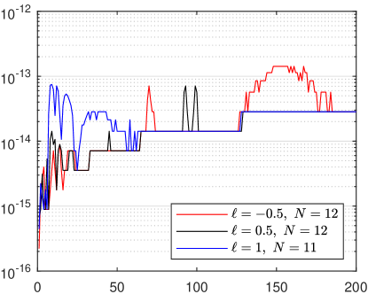
For this problem we compare the proposed method with the original NSBF representation [24, Example 7.2]. We considered three values of the parameter \ell, 1/2-1/2, 1/21/2 and 11 and computed 200 approximate eigenvalues. Absolute errors of the obtained eigenvalues are presented on Figure 2, on the left – the proposed method, on the right – the original NSBF representation. One can see the advantage of the proposed method, especially for non-integer values of \ell.

Refer to caption
Refer to caption
Figure 2: Absolute errors of the first 200 eigenvalues for the spectral problem (8.4), (8.6) for different values of \ell. On the left: the proposed representation. On the right: the original NSBF representation from [24]. On the legends the truncation parameter NN used for calculation of the approximate solution is shown next to the value of the parameter \ell.

8.3 Decay of the coefficients βn\beta_{n}

In this example we would like to illustrate numerically how far or close are the estimates of Theorem 3.5 and Corollary 3.7 from the computed decay of the coefficients βn\beta_{n}. Taking into account (1.7), estimate (3.21) states that for qW12p1[0,b]q\in W_{1}^{2p-1}[0,b] one has

n=N+1|βn(x)|2n2+3C1(x)N2+2p+2.\sum_{n=N+1}^{\infty}\frac{|\beta_{n}(x)|^{2}}{n^{2\ell+3}}\leq\frac{C_{1}(x)}{N^{2\ell+2p+2}}. (8.7)

Assuming the coefficients βn\beta_{n} are nicely behaved, one may suppose they should satisfy

|βn(x)|C2(x)np,n+p2+1.|\beta_{n}(x)|\leq\frac{C_{2}(x)}{n^{p}},\qquad n\geq\frac{\ell+p}{2}+1. (8.8)

Note that it is more like a guess and not a proven inequality. The proven inequality (3.24) is worse by a factor of n\sqrt{n}.

We considered the following potentials

qm(x)={1,xπ/2,1+(xπ/2)m,x>π/2,m=05.q_{m}(x)=\begin{cases}1,&x\leq\pi/2,\\ 1+(x-\pi/2)^{m},&x>\pi/2,\ m=0\ldots 5.\end{cases} (8.9)

It is easy to see that qmW1m[0,π]q_{m}\in W_{1}^{m}[0,\pi], but qmW1m+1[0,π]q_{m}\not\in W_{1}^{m+1}[0,\pi]. We took =1\ell=1 and for each of the potentials we computed the coefficients βk\beta_{k}, k100k\leq 100. On the left in Figure 3 we present a log-log plot of the values |βk(π)||\beta_{k}(\pi)| against kk. Such type of plot allows one to reveal dependencies of the form |βk(π)|ckα|\beta_{k}(\pi)|\sim c\cdot k^{\alpha}. The exponent α\alpha corresponds to the slope of the linear part of the curve. We obtained the following values for the exponent α\alpha (the values are reported up to 2 decimal digits).

mm 0 1 2 3 4 5
α\alpha 1.45 3.38 3.39 5.30 5.34 7.31

As one can see, the exponent indeed increases when the smoothness of the potential increases by 2, but the exponent also increases in the steps of 2 (approximately), not in the steps of 1 as predicted by (8.8). And even the decay rate for the discontinuous potential q0q_{0} is better that those that the prediction (8.8) gives for absolutely continuous potential, suggesting Theorem 4.1 may hold under weaker assumptions on qq, (2.6) may be enough.

Refer to caption
Refer to caption
Figure 3: Log-log plots of the values |βk(π)||\beta_{k}(\pi)| against kk. On the left: for different potentials qmq_{m} given by (8.9). On the right: for the potential q(x)=xq(x)=\sqrt{x} but for different values of \ell.

To verify the dependence of the decay of the coefficients βn\beta_{n} on \ell, we considered the potential q(x)=xq(x)=\sqrt{x} and computed the coefficients βk\beta_{k}, k100k\leq 100 for different values of \ell. On the right in Figure 3 we present a log-log plot of the values |βk(π)||\beta_{k}(\pi)| against kk. As one can see, the exponents α\alpha in the dependencies |βk(π)|ckα|\beta_{k}(\pi)|\sim c\cdot k^{\alpha} are essentially the same and do not depend on \ell.

Appendix A Continuous dependence of regular solutions and integral kernels on potentials

Many proofs related to transmutation operators are performed for smooth potentials and are followed by a phrase “considering an approximation by smooth potentials and passing to the limit” to show the validity for not so smooth potentials. However we are not aware of a rigorous result showing continuous dependence of the integral kernel on the potential for perturbed Bessel equations with potentials satisfying condition (2.6). For that reason we decided to include the proof in the present paper.

Consider two equations

yi′′+(+1)x2yi+qi(x)yi=ω2yi,i=1,2,x(0,b],-y_{i}^{\prime\prime}+\frac{\ell(\ell+1)}{x^{2}}y_{i}+q_{i}(x)y_{i}=\omega^{2}y_{i},\qquad i=1,2,\ x\in(0,b], (A.1)

where potentials q1q_{1} and q2q_{2} are complex valued functions satisfying condition (2.6). Without loss of generality we may assume that the parameter μ\mu is equal for both potentials.

Let yi(ω,x)y_{i}(\omega,x), i=1,2i=1,2 denote regular solutions of (A.1) satisfying the asymptotics (2.2). We are going to estimate y1(,x)y2(,x)L2()\|y_{1}(\cdot,x)-y_{2}(\cdot,x)\|_{L_{2}(\mathbb{R})} for each fixed x>0x>0. Following the notations from [17] and according to [17, Lemma 2.2], solutions y1,2y_{1,2} satisfy the integral equations

yi(ω,x)=b(ωx)+0xG(ω,x,t)qi(t)yi(ω,t)𝑑t,y_{i}(\omega,x)=b_{\ell}(\omega x)+\int_{0}^{x}G_{\ell}(\omega,x,t)q_{i}(t)y_{i}(\omega,t)\,dt,

where G(ω,x,t)G_{\ell}(\omega,x,t) is Green’s function of the initial value problem. Hence their difference satisfies the equation

y1(ω,x)y2(ω,x)\displaystyle y_{1}(\omega,x)-y_{2}(\omega,x) =0xG(ω,x,t)(q1(t)y1(ω,t)q2(t)y2(ω,t))𝑑t\displaystyle=\int_{0}^{x}G_{\ell}(\omega,x,t)\bigl{(}q_{1}(t)y_{1}(\omega,t)-q_{2}(t)y_{2}(\omega,t)\bigr{)}\,dt
=0xG(ω,x,t)(q1(t)q2(t))y1(ω,t)𝑑t\displaystyle=\int_{0}^{x}G_{\ell}(\omega,x,t)\bigl{(}q_{1}(t)-q_{2}(t)\bigr{)}y_{1}(\omega,t)\,dt
+0xG(ω,x,t)q2(t)(y1(ω,t)y2(ω,t))𝑑t.\displaystyle\quad+\int_{0}^{x}G_{\ell}(\omega,x,t)q_{2}(t)\bigl{(}y_{1}(\omega,t)-y_{2}(\omega,t)\bigr{)}\,dt. (A.2)

The following estimates hold [17, (A.1), (A.2) and (2.18)] for all ω\omega\in\mathbb{R}

|G(ω,x,t)|\displaystyle|G_{\ell}(\omega,x,t)| {C(xb+|ω|x)+1(b+|ω|tt),>1/2,C(xt(b+|ω|x)(b+|ω|t))1/2(1logtb),=1/2,\displaystyle\leq\begin{cases}C\left(\frac{x}{b+|\omega|x}\right)^{\ell+1}\left(\frac{b+|\omega|t}{t}\right)^{\ell},&\ell>-1/2,\\ C\left(\frac{xt}{(b+|\omega|x)(b+|\omega|t)}\right)^{1/2}\left(1-\log\frac{t}{b}\right),&\ell=-1/2,\end{cases}
|y1(ω,x)|\displaystyle|y_{1}(\omega,x)| Cq1(|ω|xb+|ω|x)+1(1+0xsq~1(s)b+|ω|s𝑑s)C~q1(|ω|xb+|ω|x)+1,\displaystyle\leq C_{q_{1}}\left(\frac{|\omega|x}{b+|\omega|x}\right)^{\ell+1}\biggl{(}1+\int_{0}^{x}\frac{s\tilde{q}_{1}(s)}{b+|\omega|s}\,ds\biggr{)}\leq\tilde{C}_{q_{1}}\left(\frac{|\omega|x}{b+|\omega|x}\right)^{\ell+1},

where q~1\tilde{q}_{1} is defined in (2.5) and the constant C~q1\tilde{C}_{q_{1}} can be bounded by

C~q1Cexp(Cb0xtq~1(t)𝑑t).\tilde{C}_{q_{1}}\leq C\exp\biggl{(}\frac{C}{b}\int_{0}^{x}t\tilde{q}_{1}(t)\,dt\biggr{)}.

Suppose initially that >1/2\ell>-1/2. We obtain from (A.2) that

|y1(ω,x)y2(ω,x)|CC~q1(|ω|xb+|ω|x)+10xs|q1(s)q2(s)|b+|ω|s𝑑s+C(xb+|ω|x)+10x(b+|ω|tt)|q2(t)||y1(ω,t)y2(ω,t)|𝑑t.\begin{split}|y_{1}(\omega,x)-y_{2}(\omega,x)|&\leq C\tilde{C}_{q_{1}}\left(\frac{|\omega|x}{b+|\omega|x}\right)^{\ell+1}\int_{0}^{x}\frac{s|q_{1}(s)-q_{2}(s)|}{b+|\omega|s}\,ds\\ &\quad+C\left(\frac{x}{b+|\omega|x}\right)^{\ell+1}\int_{0}^{x}\left(\frac{b+|\omega|t}{t}\right)^{\ell}|q_{2}(t)|\cdot|y_{1}(\omega,t)-y_{2}(\omega,t)|\,dt.\end{split} (A.3)

Let us divide (A.3) by (xb+|ω|x)+1\bigl{(}\frac{x}{b+|\omega|x}\bigr{)}^{\ell+1} to obtain

(b+|ω|xx)+1|y1(ω,x)y2(ω,x)|CC~q1|ω|+10xs|q1(s)q2(s)|b+|ω|s𝑑s+C0xt|q2(t)|b+|ω|t(b+|ω|tt)+1|y1(ω,t)y2(ω,t)|𝑑t.\begin{split}\left(\frac{b+|\omega|x}{x}\right)^{\ell+1}&|y_{1}(\omega,x)-y_{2}(\omega,x)|\leq C\tilde{C}_{q_{1}}|\omega|^{\ell+1}\int_{0}^{x}\frac{s|q_{1}(s)-q_{2}(s)|}{b+|\omega|s}\,ds\\ &\quad+C\int_{0}^{x}\frac{t|q_{2}(t)|}{b+|\omega|t}\cdot\left(\frac{b+|\omega|t}{t}\right)^{\ell+1}|y_{1}(\omega,t)-y_{2}(\omega,t)|\,dt.\end{split} (A.4)

The first term after “\leq” sign is a non-decreasing function. The function |y1(ω,x)y2(ω,x)|x\frac{|y_{1}(\omega,x)-y_{2}(\omega,x)|}{x^{\ell}} is continuous on [0,b][0,b] due to asymptotic condition (2.2). Hence applying Grönwall’s inequality we obtain that

(b+|ω|xx)+1|y1(ω,x)y2(ω,x)|CC~q1|ω|+10xs|q1(s)q2(s)|b+|ω|s𝑑sexp(C0xt|q2(t)|b+|ω|t𝑑t),\left(\frac{b+|\omega|x}{x}\right)^{\ell+1}|y_{1}(\omega,x)-y_{2}(\omega,x)|\leq C\tilde{C}_{q_{1}}|\omega|^{\ell+1}\int_{0}^{x}\frac{s|q_{1}(s)-q_{2}(s)|}{b+|\omega|s}\,ds\cdot\exp\biggl{(}C\int_{0}^{x}\frac{t|q_{2}(t)|}{b+|\omega|t}\,dt\biggr{)},

or

|y1(ω,x)y2(ω,x)|CC~q1(|ω|xb+|ω|x)+1exp(Cb0xt|q2(t)|𝑑t)0xs|q1(s)q2(s)|b+|ω|s𝑑s.|y_{1}(\omega,x)-y_{2}(\omega,x)|\leq C\tilde{C}_{q_{1}}\left(\frac{|\omega|x}{b+|\omega|x}\right)^{\ell+1}\exp\biggl{(}\frac{C}{b}\int_{0}^{x}t|q_{2}(t)|\,dt\biggr{)}\int_{0}^{x}\frac{s|q_{1}(s)-q_{2}(s)|}{b+|\omega|s}\,ds.

The proof for the case =1/2\ell=-1/2 is completely similar, the additional factor 1logtb1-\log\frac{t}{b} results in the change of q1q_{1} and q2q_{2} by q~1\tilde{q}_{1} and q~2\tilde{q}_{2}. Combining we obtain the following estimate

|y1(ω,x)y2(ω,x)|CC~q1(|ω|xb+|ω|x)+1exp(Cb0xt|q~2(t)|𝑑t)0xs|q~1(s)q~2(s)|b+|ω|s𝑑s.|y_{1}(\omega,x)-y_{2}(\omega,x)|\leq C\tilde{C}_{q_{1}}\left(\frac{|\omega|x}{b+|\omega|x}\right)^{\ell+1}\exp\biggl{(}\frac{C}{b}\int_{0}^{x}t|\tilde{q}_{2}(t)|\,dt\biggr{)}\int_{0}^{x}\frac{s|\tilde{q}_{1}(s)-\tilde{q}_{2}(s)|}{b+|\omega|s}\,ds. (A.5)

Let us introduce the notation

C(q,x):=Cexp(Cb0xt|q~|dt).C(q,x):=C\exp\biggl{(}\frac{C}{b}\int_{0}^{x}t|\tilde{q}|\,dt\biggl{)}.
Theorem A.1.

Let the potentials q1q_{1} and q2q_{2} satisfy condition (2.6) with the same exponent μ\mu and let y1,2y_{1,2} be regular solutions of (A.1) satisfying asymptotics (2.2). Then for each x(0,b]x\in(0,b]

y1(,x)y2(,x)L2()cμC(q1,x)C(q2,x)0xtμ|q~1(t)q~2(t)|𝑑t,\|y_{1}(\cdot,x)-y_{2}(\cdot,x)\|_{L_{2}(\mathbb{R})}\leq c_{\mu}C(q_{1},x)C(q_{2},x)\int_{0}^{x}t^{\mu}|\tilde{q}_{1}(t)-\tilde{q}_{2}(t)|\,dt,

where the constant cμc_{\mu} does not depend on the potentials.

Proof.

It follows from (A.5) that for |μ|>1|\mu|>1

|y1(ω,x)y2(ω,x)|C(q1,x)C(q2,x)0xtμ|q~1(t)q~2(t)|(tb+|ω|t)1μ(1b+|ω|t)μ𝑑tC(q1,x)C(q2,x)1|ω|1μ1bμ0xtμ|q~1(t)q~2(t)|𝑑t\begin{split}|y_{1}(\omega,x)-y_{2}(\omega,x)|&\leq C(q_{1},x)C(q_{2},x)\int_{0}^{x}t^{\mu}|\tilde{q}_{1}(t)-\tilde{q}_{2}(t)|\cdot\left(\frac{t}{b+|\omega|t}\right)^{1-\mu}\left(\frac{1}{b+|\omega|t}\right)^{\mu}dt\\ &\leq C(q_{1},x)C(q_{2},x)\frac{1}{|\omega|^{1-\mu}}\frac{1}{b^{\mu}}\int_{0}^{x}t^{\mu}|\tilde{q}_{1}(t)-\tilde{q}_{2}(t)|\,dt\end{split}

and for |μ|1|\mu|\leq 1

|y1(ω,x)y2(ω,x)|C(q1,x)C(q2,x)(xb)1μ1bμ0xtμ|q~1(t)q~2(t)|𝑑t.|y_{1}(\omega,x)-y_{2}(\omega,x)|\leq C(q_{1},x)C(q_{2},x)\left(\frac{x}{b}\right)^{1-\mu}\frac{1}{b^{\mu}}\int_{0}^{x}t^{\mu}|\tilde{q}_{1}(t)-\tilde{q}_{2}(t)|\,dt.

Combining the last two inequalities the statement follows. ∎

Corollary A.2.

Let the potentials q1q_{1} and q2q_{2} satisfy condition (2.6) with the same exponent μ\mu and let K1,2K_{1,2} be corresponding integral kernels of the transmutation operators. Then for each x(0,b]x\in(0,b]

K1(x,)K2(x,)L2(0,b)cμ2C(q1,x)C(q2,x)0xtμ|q~1(t)q~2(t)|𝑑t.\|K_{1}(x,\cdot)-K_{2}(x,\cdot)\|_{L_{2}(0,b)}\leq\frac{c_{\mu}}{2}C(q_{1},x)C(q_{2},x)\int_{0}^{x}t^{\mu}|\tilde{q}_{1}(t)-\tilde{q}_{2}(t)|\,dt.
Proof.

Recall that for each fixed xx the integral kernels K1K_{1} and K2K_{2} are the Hankel transforms of the solutions y1y_{1} and y2y_{2} from Theorem A.1 [34, Theorem 2.4]. Hence

K1(x,t)K2(x,t)=0(y1(ω,x)y2(ω,x))ωtJ+1/2(ωt)𝑑t.K_{1}(x,t)-K_{2}(x,t)=\int_{0}^{\infty}\bigl{(}y_{1}(\omega,x)-y_{2}(\omega,x)\bigr{)}\sqrt{\omega t}J_{\ell+1/2}(\omega t)\,dt.

Now the statement follows from Parseval’s equality for the Hankel transform. ∎

Consider the function

ν(x)={xμ,>1/2,xμ(1logxb),=1/2.\nu(x)=\begin{cases}x^{\mu},&\ell>-1/2,\\ x^{\mu}(1-\log\frac{x}{b}),&\ell=-1/2.\end{cases}

Then potential qq satisfies condition (2.6) if and only if qL1((0,b),ν(x)dx)q\in L_{1}\bigl{(}(0,b),\nu(x)\,dx\bigr{)}.

Corollary A.3.

Let the potential qq satisfy condition (2.6) with a parameter μ\mu and let {qn}n=0L1((0,b),ν(x)dx)\{q_{n}\}_{n=0}^{\infty}\subset L_{1}\bigl{(}(0,b),\nu(x)\,dx\bigr{)} be a sequence of potentials such that

qnL1((0,b),ν(x)dx)q,n.q_{n}\overset{L_{1}((0,b),\nu(x)\,dx)}{\longrightarrow}q,\qquad n\to\infty. (A.6)

Let KK, R~\tilde{R} and KnK_{n}, R~n\tilde{R}_{n} be corresponding integral kernels. Then for any x>0x>0

Kn(x,)L2(0,x)K(x,)andRn(x,)L2(x,x)R(x,),n.K_{n}(x,\cdot)\overset{L_{2}(0,x)}{\longrightarrow}K(x,\cdot)\qquad\text{and}\qquad R_{n}(x,\cdot)\overset{L_{2}(-x,x)}{\longrightarrow}R(x,\cdot),\quad n\to\infty.
Proof.

It follows from (A.6) that the quantities C(qn,x)C(q_{n},x) are uniformly bounded by 2C(q,x)2C(q,x) for all nn0n\geq n_{0}. Hence the convergence Kn(x,)K(x,)K_{n}(x,\cdot)\to K(x,\cdot) follows immediately from Corollary A.2.

Recall that the integral kernel RR is the Fourier transform of the regular solution y~\tilde{y} satisfying the asymptotics y~(ω,x)x+1\tilde{y}(\omega,x)\sim x^{\ell+1} at 0. Dividing (A.5) by ω+1\omega^{\ell+1} we obtain that

|y~(ω,x)y~n(ω,x)|C(q,x)C(qn,x)(xb+|ω|x)+10xs|q~1(s)q~2(s)|b+|ω|s𝑑s.|\tilde{y}(\omega,x)-\tilde{y}_{n}(\omega,x)|\leq C(q,x)C(q_{n},x)\left(\frac{x}{b+|\omega|x}\right)^{\ell+1}\int_{0}^{x}\frac{s|\tilde{q}_{1}(s)-\tilde{q}_{2}(s)|}{b+|\omega|s}\,ds.

Using the last inequality one can prove that Rn(x,)R(x,)R_{n}(x,\cdot)\to R(x,\cdot) following the proof for the kernels KK and KnK_{n} with minimal changes. ∎

Appendix B On existence of non-vanishing particular solution

Problem of existence of a non-vanishing particular solution of a differential equation naturally arises in the construction of coefficients for both SPPS [22, 7] and Neumann series of Bessel functions [21, 24] representations for solutions. While for a non-singular case it is always possible to choose such linear combination of linearly independent particular solutions that it will not vanish on the whole interval of interest (see [22, Remark 5], see also [5]), a perturbed Bessel equation possesses only one (up to a multiplicative constant) regular solution which either vanishes at some point or not. In this appendix we show that at least it is always possible to perform such spectral shift, i.e., consider an equation

u′′+((+1)x2+q(x)+λ)u=0,-u^{\prime\prime}+\left(\frac{\ell(\ell+1)}{x^{2}}+q(x)+\lambda\right)u=0, (B.1)

that its regular solution will be non-vanishing on (0,b](0,b].

In some situations such value of λ\lambda is easy to choose. For example, if qq is real valued and bounded from below, any λinf(0,b]q(x)\lambda\geq-\inf_{(0,b]}q(x) works, see, e.g., [7, Corollary 3.3]. For real valued potentials any λ\lambda having Imλ0\operatorname{Im}\lambda\neq 0 works since the equality u(x0)=0u(x_{0})=0 would imply the existence of imaginary eigenvalue for selfadjoint problem (B.1) with Dirichlet boundary conditions formulated on [0,x0][0,x_{0}], c.f., [8, Remark 4.1]. Lemma 3.1 from [6] shows that for real valued potentials satisfying qL2(0,b)q\in L_{2}(0,b) any λ\lambda satisfying λ0b|q(x)|2𝑑x\lambda\geq\int_{0}^{b}|q(x)|^{2}\,dx works.

The following proposition shows the existence of such λ\lambda for any potential satisfying

xq(x)L1(0,b)if >1/2,xq(x)(1logxb)L1(0,b)if =1/2.\begin{split}xq(x)&\in L_{1}(0,b)\qquad\text{if }\ell>-1/2,\\ xq(x)\Bigl{(}1-\log\frac{x}{b}\Bigr{)}&\in L_{1}(0,b)\qquad\text{if }\ell=-1/2.\end{split} (B.2)
Proposition B.1.

Let qq be complex valued function satisfying condition (B.2). Then there exist such constant λ0>0\lambda_{0}>0 that for all λ>λ0\lambda>\lambda_{0} the regular solution of equation (B.1) does not vanish on (0,b](0,b].

Proof.

Let λ=ω2\lambda=\omega^{2}, ω>0\omega>0. The regular solution of (B.1) can be written in the form

u(x,ω)=ωxI+1/2(ωx)+r(ω,x),u(x,\omega)=\sqrt{\omega x}I_{\ell+1/2}(\omega x)+r(\omega,x),

where I+1/2I_{\ell+1/2} is the modified Bessel function of the first kind. The function r(ω,x)r(\omega,x) satisfies, see [17, Lemma 2.2]

|r(ω,x)|C(ωxb+ωx)+1eωx0xyq~(y)b+ωy𝑑y,|r(\omega,x)|\leq C\left(\frac{\omega x}{b+\omega x}\right)^{\ell+1}e^{\omega x}\int_{0}^{x}\frac{y\tilde{q}(y)}{b+\omega y}\,dy,

where the constant CC does not depend on ω\omega; q~(y)=|q(y)|\tilde{q}(y)=|q(y)| if >1/2\ell>-1/2 and q~(y)=|q(y)|[1log(y/b)]\tilde{q}(y)=|q(y)|[1-\log(y/b)] if =1/2\ell=-1/2.

Due to the asymptotics Iν(z)ez2πzI_{\nu}(z)\sim\frac{e^{z}}{\sqrt{2\pi z}}, zz\to\infty [1, (9.7.1)], there exists such z0z_{0} that I+1/2(z)ez4zI_{\ell+1/2}(z)\geq\frac{e^{z}}{4\sqrt{z}} for all zz0z\geq z_{0}. Let z1:=max{z0,8C0byq~(y)𝑑y}z_{1}:=\max\{z_{0},8C\int_{0}^{b}y\tilde{q}(y)\,dy\} (the integral is finite due to the condition (B.2)) and let x0>0x_{0}>0 be such that 0x0yq~(y)𝑑y<b/8C\int_{0}^{x_{0}}y\tilde{q}(y)\,dy<b/8C.

If ωxz1\omega x\geq z_{1} and ωz1/x0\omega\geq z_{1}/x_{0}, then

|r(ω,x)|<Ceωxb0x0yq~(y)𝑑y+Ceωxωx0x0xyq~(y)𝑑yeωx4ωxI+1/2(ωx)|r(\omega,x)|<\frac{Ce^{\omega x}}{b}\int_{0}^{x_{0}}y\tilde{q}(y)\,dy+\frac{Ce^{\omega x}}{\omega x_{0}}\int_{x_{0}}^{x}y\tilde{q}(y)\,dy\leq\frac{e^{\omega x}}{4}\leq\sqrt{\omega x}I_{\ell+1/2}(\omega x)

and hence u(x,ω)0u(x,\omega)\neq 0.

Let 0<ωx<z10<\omega x<z_{1}. We may estimate the function I+1/2I_{\ell+1/2} by the first term of its Taylor series, i.e.,

ωxI+1/2(ωx)(ωx)+12+1/2Γ(+3/2),0<ωx<z1.\sqrt{\omega x}I_{\ell+1/2}(\omega x)\geq\frac{(\omega x)^{\ell+1}}{2^{\ell+1/2}\Gamma(\ell+3/2)},\qquad 0<\omega x<z_{1}.

Since yq~(y)L1(0,b)y\tilde{q}(y)\in L_{1}(0,b), there exists x1>0x_{1}>0 such that

0x1yq~(y)𝑑yb+22+1/2Γ(+3/2)Cez1.\int_{0}^{x_{1}}y\tilde{q}(y)\,dy\leq\frac{b^{\ell+2}}{2^{\ell+1/2}\Gamma(\ell+3/2)Ce^{z_{1}}}.

Take ωz1/x1\omega\geq z_{1}/x_{1}. Then it follows from the inequality ωx<z1\omega x<z_{1} that x<x1x<x_{1}. Hence

|r(ω,x)|<Cez1(ωx)+1b+20x1yq~(y)𝑑yωxI+1/2(ωx),|r(\omega,x)|<\frac{Ce^{z_{1}}(\omega x)^{\ell+1}}{b^{\ell+2}}\int_{0}^{x_{1}}y\tilde{q}(y)\,dy\leq\sqrt{\omega x}I_{\ell+1/2}(\omega x),

and so u(x,ω)0u(x,\omega)\neq 0.

Hence for all values of ω\omega greater than max{z1x0,z1x1}\max\bigl{\{}\frac{z_{1}}{x_{0}},\frac{z_{1}}{x_{1}}\bigr{\}} the function u(x,ω)u(x,\omega) does not vanish on (0,b](0,b]. ∎

References

  • [1] M. Abramovitz and I. A. Stegun, Handbook of mathematical functions, New York: Dover, 1972.
  • [2] R. A. Adams, Sobolev Spaces. Pure and Applied Mathematics, Vol. 65, New York–London: Academic Press, 1975.
  • [3] A. Baricz, D. Jankov and T. K. Pogány, Neumann series of Bessel functions, Integral Transforms Spec. Funct. 23 (2012), no. 7, 529–538.
  • [4] A. Boumenir and B. Chanane, Computing eigenvalues of Sturm-Liouville systems of Bessel type, P. Edinburgh Math. Soc. 42 (1999), 257–265.
  • [5] R. Camporesi and A. J. Di Scala, A generalization of a theorem of Mammana, Colloq. Math. 122 (2011), no. 2, 215–223.
  • [6] R. Carlson, Inverse spectral theory for some singular Sturm-Liouville problems, J. Differ. Equations 106 (1993), 121–140.
  • [7] R. Castillo-Pérez, V. V. Kravchenko and S. M. Torba, Spectral parameter power series for perturbed Bessel equations, Appl. Math. Comput. 220 (2013), 676–694.
  • [8] R. Castillo-Pérez, V. V. Kravchenko and S. M. Torba, Analysis of graded-index optical fibers by the spectral parameter power series method, J. Optics 17 (2015), 025607 (9pp).
  • [9] H. Chébli, A. Fitouhi and M. M. Hamza, Expansion in series of Bessel functions and transmutations for perturbed Bessel operators, J. Math. Anal. Appl. 181 (1994), no. 3, 789–802.
  • [10] M. Coz and Ch. Coudray, The Riemann solution and the inverse quantum mechanical problem, J. Math. Phys. 17 (1976), no. 6, 888–893.
  • [11] B. B. Delgado, K. V. Khmelnytskaya, V. V. Kravchenko, The transmutation operator method for efficient solution of the inverse Sturm-Liouville problem on a half-line, Math. Meth. Appl. Sci. 42 (2019) 7359–7366.
  • [12] R. Devore and G. Lorentz, Constructive approximation, Berlin: Springer-Verlag, 1993.
  • [13] J. L. Griffith, Hankel transforms of functions zero outside a finite interval, J. Proc. Roy. Soc. New South Wales 89 (1955), 109–115.
  • [14] J.-C. Guillot and J. V. Ralston, Inverse spectral theory for a singular Sturm-Liouville operator on [0,1], J. Differ. Equations 76 (1988), no. 2, 353–373.
  • [15] A. Fitouhi and M. M. Hamza, A uniform expansion for the eigenfunction of a singular second-order differential operator, SIAM J. Math. Anal. 21 (1990), 1619–1632.
  • [16] M. Holzleitner, Transformation operators for spherical Schrödinger operators, J. Math. Anal. Appl. 481 (2020), no. 1, 123430, 27 pp.
  • [17] A. Kostenko, A. Sakhnovich and G. Teschl, Inverse eigenvalue problems for perturbed spherical Schrödinger operators, Inverse Problems 26 (2010), 105013 (14pp).
  • [18] A. Kostenko and G. Teschl, On the singular Weyl-Titchmarsh function of perturbed spherical Schrödinger operators, J. Differ. Equations 250 (2011), 3701–3739.
  • [19] V. V. Kravchenko, On a method for solving the inverse Sturm–Liouville problem, J. Inverse Ill-pose P. 27 (2019), 401–407.
  • [20] V. V. Kravchenko, Direct and inverse Sturm-Liouville problems: A method of solution, Birkhäuser, Basel, 2020.
  • [21] V. V. Kravchenko, L. J. Navarro and S. M. Torba, Representation of solutions to the one-dimensional Schrödinger equation in terms of Neumann series of Bessel functions, Appl. Math. Comput. 314 (2017), 173–192.
  • [22] V. V. Kravchenko and R. M. Porter, Spectral parameter power series for Sturm–Liouville problems, Math. Meth. Appl. Sci. 33 (2010), 459–468.
  • [23] V. V. Kravchenko, E. L. Shishkina and S. M. Torba, On a series representation for integral kernels of transmutation operators for perturbed Bessel equations, Math. Notes 104 (2018), 552–570.
  • [24] V. V. Kravchenko, S. M. Torba and R. Castillo-Pérez, A Neumann series of Bessel functions representation for solutions of perturbed Bessel equations, Appl. Anal. 97 (2018), 677–704.
  • [25] V. V. Kravchenko, S. M. Torba and J. Yu. Santana-Bejarano, Generalized wave polynomials and transmutations related to perturbed Bessel equations, Math. Meth. Appl. Sci. 42 (2019), 5008–5028.
  • [26] N. X. Ky, On weighted polynomial approximation with a weight (1x)α/2(1+x)β/2(1-x)^{\alpha/2}(1+x)^{\beta/2} in L2L_{2}-space, Acta Math. Hung. 27 (1976), no. 1-2, 101–107.
  • [27] V. Ledoux and M. Van Daele, Matslise 2.0: A Matlab toolbox for Sturm-Liouville computations, ACM Trans. Math. Softw. 42 (2016), 29:1–18.
  • [28] F. Móricz, Absolutely convergent Fourier integrals and classical function spaces, Arch. Math. 91 (2008), 49–62.
  • [29] K. Okamoto, Fundamentals of optical waveguides, San Diego: Academic Press, 2000.
  • [30] A. P. Prudnikov, Yu. A. Brychkov and O. I. Marichev, Integrals and series. Vol. 2. Special functions, New York: Gordon & Breach Science Publishers, 1986, 750 pp.
  • [31] G. Sampson and H. Tuy, Fourier transforms and their Lipschitz classes, Pac. J. Math. 75 (1978), no. 2, 519–537.
  • [32] S. M. Sitnik and E. L. Shishkina, Method of transmutaitons for differential equations with Bessel operators, Moskow: Fizmatlit, 2019 (in Russian).
  • [33] A. S. Sohin, The inverse scattering problem for an equation with a singularity (in Russian), Mat. Fiz. i Funkcional. Anal. 2 (1971), 182–235.
  • [34] V. V. Stashevskaya, On the inverse problem of spectral analysis for a differential operator with a singularity at zero (in Russian), Zap. Mat. Otdel. Fiz.-Mat.Fak.KhGU i KhMO 25 (4) (1957) 49–86.
  • [35] P. K. Suetin, Classical orthogonal polynomials, 3rd ed. (in Russian), Moscow: Fizmatlit, 2005, 480 pp.
  • [36] G. Szegö, Orthogonal Polynomials, revised edition, New York: American Mathematical Society, 1959.
  • [37] K. Trimeche, Transmutation operators and mean-periodic functions associated with differential operators, Harwood Academic Publishers, 1988.
  • [38] V. Ya. Volk, On inversion formulas for a differential equation with a singularity at x=0x=0, Uspehi Matem. Nauk (N.S.) 8 (1953). no. 4(56), 141–151.
  • [39] J. Weidmann, Spectral Theory of Ordinary Differential Operators, Lecture Notes in Math., Berlin: Springer, 1987.
  • [40] J. E. Wilkins, Neumann series of Bessel functions, Trans. Amer. Math. Soc. 64 (1948), 359–385.