Translators of the Gauss curvature flow

The flow by powers of the Gauss curvature $K$ was initiated by Chow [8] after the articles of Firey and Tso ([11, 15]). These works were the starting point of the theory of the flow by the Gaussian curvature ([1, 16]), a topic of high activity in geometric analysis that continues to the present. Given a smooth immersion $X:\Sigma\to\mathbb{R}^{3}$ of a strictly convex surface $\Sigma$ in Euclidean space $\mathbb{R}^{3}$, we consider the $K^{\alpha}$-flow as a one-parameter family of smooth immersions $X_{t}=X(\cdot,t)\colon\Sigma\to\mathbb{R}^{3}$, $t\in[0,T)$ such that $X_{0}=X$ and satisfying the flow

where $\alpha\in\mathbb{R}$ is a constant, $N(p,t)$ is the unit normal of $X(p,t)$ and $K(p,t)$ is the Gauss curvature at $X(p,t)$. An interesting problem is the evolution of a surface through the flow. As an example for the reader, if $\alpha=1$ the surface becomes spherical ([3]).

If the surface moves under the $K^{\alpha}$-flow along a spatial direction $\vec{v}\in\mathbb{R}^{3}$, then $X_{0}$ satisfies $K^{\alpha}=\lambda\langle N,\vec{v}\rangle$ for some positive constant $\lambda$. The vector $\vec{v}$ is assumed to be unitary and it is called the speed of the flow. After a dilation, we can assume that $\lambda=1$. A surface $\Sigma$ is called a translator by the $K^{\alpha}$-flow with speed $\vec{v}$, or simply, a $K^{\alpha}$-translator in case that $\vec{v}$ is understood, if

The notion of translator by positive powers of the Gauss curvature appeared in [17]. See also [9, 14].

In this paper we want to find examples of $K^{\alpha}$-translators under the geometric condition that the surface is defined kinematically as the movement of a curve by a uniparametric family of rigid motions of $\mathbb{R}^{3}$. Following Darboux [10, Livre I], we consider surfaces parametrized by $\Psi(s,t)=A(t)\cdot\gamma(s)+\beta(t)$, where $\gamma$ and $\beta$ are two spatial curves and $A(t)$ is an orthogonal matrix. The cases that we are interesting are: rotational surfaces ($A(t)$ is a uniparametric group of rotations and $\beta$ is constant), helicoidal surfaces ($A(t)$ is a uniparametric group of helicoidal motions), translation surfaces ($A(t)$ is the identity) and ruled surfaces ($\gamma$ is a straight-line). Since we have left to one side the study of the evolution of the surface, we do not require that $K$ to be positive but only that $K^{\alpha}$ has sense. For example, $K$ may be negative if $\alpha\in\mathbb{Z}$. This will be implicitly assumed in all the results.

In the flow by powers of the Gaussian curvature, it is known that the $K^{1/4}$-flow is special because it has an interpretation in affine differential geometry as the affine normal flow of a convex surface ([2, 6]). However, in base of our proofs, this case will appear as natural because when we express the equation (1) for each one of the above three types of surfaces and when $\alpha$ is exactly $1/4$, this equation is greatly simplified due to a cancellation of terms. This makes the arguments easier than in the general case of $\alpha$.

Planes are examples of $K^{\alpha}$-translators for any $\alpha>0$ provided the plane is parallel to the speed of the flow. Throughout this paper, we will discard planes as examples of $K^{\alpha}$-translators. Other examples that we will not consider in the class of $K^{\alpha}$-translators are the surfaces whose Gauss curvature is constant, where now the equation (1) says that the unit normal vector $N$ makes a constant angle with a fixed direction. Similarly, we discard the case $\alpha=0$.

It is important to point out that there is not a priori relation between the speed vector $\vec{v}$ and the special parametrization of each of the above Darboux surfaces. So, if one considers the study of translators one can prescribed the speed $\vec{v}$, usually, the vector $(0,0,1)$ in the literature. However, if one considers one of the above types of Darboux surfaces, the parametrization has no relation with $\vec{v}$. This can be clearly seen for rotational surfaces (also helicoidal surfaces). The rotation axis of the surface is, initially, independent of the vector $\vec{v}$. However, as we will see, for rotational and helicoidal surfaces, the speed must be parallel to the axis (Propositions 2.1 and 3.1). Something similar occurs for translations surfaces where, if one prescribes that the surface is $z=f(x)+g(y)$, the speed may be arbitrary.

The organization of this paper is as follows. In Section 2, we obtain all rotational $K^{\alpha}$-translators. Recall that in [17], Urbas obtains these surfaces for $\alpha\in(0,1/2]$ using the Legendre transform (see also [13] for a similar calculation). Our approach uses simple geometric arguments and it holds for any $\alpha$ (Theorem 2.2). In particular, for each value of $\alpha$, we prove the existence of rotational examples intersecting orthogonally the rotation axis (Corollary 2.4). Section 3 is devoted to the study of $K^{\alpha}$-translators of helicoidal type. Although we are not able to obtain explicit parametrizations of these surfaces, we do a first integration of the generating curve (Theorem 3.2), also in terms of the Bour function (Theorem 3.3). In Section 4, we obtain the classification of all solutions of (1) obtained by separation of variables $z=f(x)+g(y)$, where $(x,y,z)$ are the canonical coordinate system of $\mathbb{R}^{3}$. Although these solutions depend on a particular choice of coordinates of $\mathbb{R}^{3}$, our result holds for any speed vector $\vec{v}$. In particular, we prove that there are $K^{\alpha}$-translators only if $\alpha=1/4$ (Theorems 4.1 and 4.3). Besides we provide new examples of $K^{1/4}$-translators of type $z=f(x)+g(y)$, we also give new examples of $K^{1/4}$-translators obtained by separation of variables of type $z=f(x)g(y)$ (Example 4.4). Finally, in Section 5, we investigate the existence of ruled $K^{\alpha}$-translators, proving that there are not ruled $K^{\alpha}$-translators, except trivial cases (Theorem 5.1).

The authors have extended the results of this paper for (spacelike and timelike) $K^{\alpha}$-translators in Lorentz-Minkowski space ([4]).

In this section, we classify the surfaces of revolution satisfying (1). A first question is if there is a relation between the rotation axis of the surface and the speed vector $\vec{v}$. As it is expectable, we prove that the vector $\vec{v}$ must be parallel to the rotation axis.

After a rigid motion, we will assume that the rotation axis is the $z$-axis and consequently from this proposition, that $\vec{v}=(0,0,1)$ after a symmetry about the $xy$-plane if necessary. Then (1) is

Set $g=f^{\prime}/(1+f^{\prime 2})^{1/2}$. Notice that $\kappa_{1}=g^{\prime}$ and $r\kappa_{2}=g$. In terms of $g$, the above equation becomes

A first integration gives

In the case $\alpha=1/2$, the condition $g*2\geq 0$ says that the domain of $r$ is when $r^{2}\geq\log(m)$. Otherwise, we need to distinguish if $2\alpha/(2\alpha-1)$ is negative or positive, that is, $\alpha$ belongs to $(0,1/2)$ or not. If $\alpha\in(0,1/2)$, the parenthesis in (3) must be positive, yielding $r^{2}>2\alpha/(2\alpha-1)m$. On the other hand, using now that $g^{2}\geq 0$, we have $r^{2}\geq 2\alpha/(2\alpha-1)(m-1)\geq 0$, so this is the restriction on $r$ because $2\alpha/(2\alpha-1)<0$. If $\alpha\not\int[0,1/2]$, then $2\alpha/(2\alpha-1)>0$. Since the parenthesis in (3) must be positive because $g^{2}<1$, then we obtain $r^{2}<2\alpha/(2\alpha-1)m$ and from the fact that $g^{2}\geq 0$, the restriction is $r^{2}\geq 2\alpha/(2\alpha-1)(m-1)$. To summarize, we have

Hence we deduce

As conclusion, we have the classification of all $K^{\alpha}$-translators that also are surfaces of revolution.

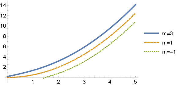
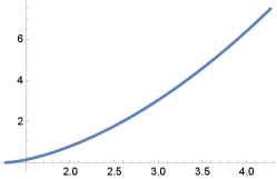
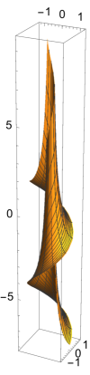
We point that it is expectable that in the case $\alpha\not\in[0,1/2]$ the domain cannot be $[0,\infty)$ because there are no entire graphs that are $K^{\alpha}$-translators if $\alpha>1/2$ ([17, Sect. 4]) and if $\alpha<0$ ([18, Th. 6.1]). It deserves to note the case $\alpha=1/4$ because it is possible to integrate explicitly (6) (see also [14]). See Figure 1.

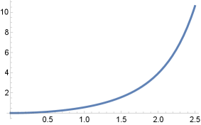
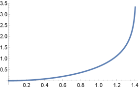
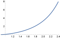
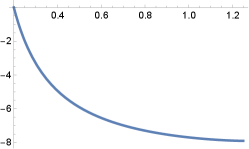
By (4), we point out that the maximal domain of $f$ is not $[0,\infty)$ in general. However, an interesting case to investigate is if there are generating curves that meet orthogonally the rotation axis. We prove that this occurs for all cases of $\alpha$. See Figure 2.

We point out that in some particular cases, the integrals in (6) can be explicitly solved. Here, we denote by $f_{\alpha}$ to emphasize the parameter $\alpha$ where we also assume $m=1$.

1. (1)

   Case $\alpha=1$. Then

   $$f^{\prime}(r)=\frac{r\sqrt{4-r^{2}}}{2-r^{2}}$$

   and

   $$f_{1}(r)=\mp\sqrt{4-r^{2}}\pm\sqrt{2}\tanh^{-1}\left(\frac{1}{\sqrt{2}}\sqrt{4-r^{2}}\right),$$

   defined on $[0,2).$

2. (2)

   Case $\alpha=1/3$. Now

   $$f^{\prime}(r)=\pm\frac{1}{2}r\sqrt{4+r^{2}}$$

   and the solution is

   $$f_{1/3}(r)=\pm\frac{1}{6}\left(4+r^{2}\right)^{3/2},$$

   defined on $[0,\infty).$

3. (3)

   For $\alpha=1/6$, we have

   $$f^{\prime}(r)=\pm(\sqrt{2r^{2}+1}-1)^{1/2},$$

   and

   $$f_{1/6}(r)=\pm\frac{\sqrt{\sqrt{2r^{2}+1}-1}\left(2r^{2}-\sqrt{2r^{2}+1}-1\right)}{3r},$$

   and defined on $[0,\infty)$.

Consider a helicoidal surface $\Sigma$ in $\mathbb{R}^{3}$ with axis $z$ whose generating curve $\gamma$ is included in the $xz$-plane and pitch $h$. Without loss of generality, we can assume that $\gamma(r)=(r,0,f(r))$ where $f\colon I\subset\mathbb{R}^{+}\to\mathbb{R}$ is a smooth function. Then $\Sigma$ parametrizes by

If $D=r^{2}(1+f^{\prime 2})+h^{2}$, then the unit normal vector $N$ is

and the Gauss curvature is

Then $\Sigma$ is a $K^{\alpha}$-translator if

As a first conclusion, we prove that $\vec{v}$ must be parallel to the $z$-axis. The proof is similar of Proposition 2.1.

From this proposition, we can assume that $\vec{v}=(0,0,1)$. Then (8) is

We will obtain a first integration of this equation. For this, let

Then $\frac{r}{2}g^{\prime}=g+r^{3}f^{\prime}f^{\prime\prime}-h^{2}$ and thus (9) is equivalent to

If $\alpha=1/2$, the solution is $g(r)=mr^{2}e^{r^{2}}$, with $m\in\mathbb{R}$. If $\alpha\not=1/2$, the solution of this equation is

In terms of the function $f$, we have

In particular, this gives a restriction on the domain of $f(r)$.

We now show examples of $f^{\prime}$ for some choices of $\alpha$. In all cases, the pitch is $h=1$. See Figures 3 and 4

1. (1)

   Case $\alpha=1/2$. We take $m=1$ in (10). The function $f$ is defined provided $r^{2}\geq\log((1+r^{2})/r^{2})$, that is, $[r_{0},\infty)$, where $r_{0}\approx 0.898$.

2. (2)

   Case $\alpha=1/4$. Let $m=0$. Then $1+f^{\prime 2}=-1/r^{2}+r^{2}$. Now the restriction on $r$ is $r^{4}-r^{2}-1\geq 0$, that is, the domain is $[r_{0},\infty)$ with $r_{0}\approx 1.272$. This case appeared in [14].

3. (3)

   Case $\alpha=1$. Let $m=0$ in (10). Then $1+f^{\prime 2}=4/r^{4}-1/r^{2}$ and the domain of $f$ is $[0,r_{0}]$ with $r_{0}\approx 1.249$. Here $\lim_{r\to 0}f(r)=\lim_{r\to 0}f^{\prime}(r)=\infty$.

Following Lee [14] we may also use the approach of Bour ([7]). More explicitly, the Bour coordinates are defined by $r\mapsto s$ and $\theta\mapsto t,$ $t=\theta+\Theta$, where

The first fundamental form is now $I=ds^{2}+U^{2}dt^{2},$ where the so-called Bour function is introduced by the relation $U^{2}=r^{2}+h^{2}.$ Using the Bour function $U$, the terms $r$, $f$ and $\Theta$ can be determined by

With the above discussion, the Gauss curvature is now $K=-(d^{2}U/ds^{2})/U$ and $\left\langle N,(0,0,1)\right\rangle=dU/ds.$ Then (1) is now

or equivalently

Setting $P=dU/ds$ and $\frac{dP}{dU}=(ds/dU)(d^{2}U/ds^{2})$, we have

A first integration is

where $m\in\mathbb{R}$ is a integration constant with $m>0$ if $\alpha=1/2$. Because $s$ can be viewed a function of $U$, we may interchange their roles. Therefore, we obtain again a classification of helicoidal $K^{\alpha}$-translators in terms of the Bour function $U$.

Again, for some particular values of $\alpha$, (12) can be explicitly integrated. We present the cases $\alpha=1/4$ ([14]), $\alpha=1/3$ and $\alpha=1$.

1. (1)

   Case $\alpha=1/4.$ The solution is

   $$s=\left\{\begin{array}[]{lll}\frac{1}{2}\left(U\sqrt{m+U^{2}}+m\cosh^{-1}(U)\right),&U\geq\{\sqrt{-m},1\}&\mbox{when }m<0,\\ \frac{1}{2}U^{2},&U>0&\mbox{when }m=0,\\ \frac{1}{2}\left(U\sqrt{m+U^{2}}+m\sinh^{-1}(U)\right),&U>0&\mbox{when }m>0.\end{array}\right.$$

2. (2)

   Case $\alpha=1/3$. The solution is

   $$s=mU+\frac{U^{3}}{6},$$

   where $U\in(0,\infty).$

3. (3)

   Case $\alpha=1.$ Then,

   $$s=\left\{\begin{array}[]{lll}\sqrt{\frac{2}{m}}\tanh^{-1}\left(\frac{U}{\sqrt{2m}}\right),&U\leq\sqrt{2m}&\mbox{when }m>0\\ \frac{2}{U},&U>0&\mbox{when }m=0\\ -\sqrt{\frac{2}{-m}}\tan^{-1}\left(\frac{U}{\sqrt{-2m}}\right),&U\leq\sqrt{-2m}&\mbox{when }m<0.\end{array}\right.$$

   In particular, we can express $U$ in terms of $s$,

   $$U=\left\{\begin{array}[]{lll}\sqrt{\frac{m}{2}}\tanh\left(\sqrt{2m}s\right),&\mid s\mid\leq(2m)^{-1/2}&\mbox{when }m>0\\ \frac{2}{s},&s>0&\mbox{when }m=0\\ -\sqrt{\frac{-m}{2}}\tan\left(\sqrt{-2m}s\right),&\mid s\mid\leq(-2m)^{-1/2}&\mbox{when }m<0.\end{array}\right.$$

By a translation surface of $\mathbb{R}^{3}$ we mean a surface given by the sum of two curves contained in two coordinate planes. This is a particular case of a Darboux surface where $A(t)$ is the identity. After a rigid motion, the surface is the sum of the curves $\gamma(x)=(x,0,f(x))$ and $\beta(y)=(0,y,g(y))$, where $f\colon I\subset\mathbb{R}\to\mathbb{R}$ and $g\colon J\subset\mathbb{R}\to\mathbb{R}$ are smooth functions in one variable. Thus the surface parametrizes by

If we see the surface $\Sigma$ as the graph of $z=f(x)+g(y)$, then the problem of finding all translation surfaces that are $K^{\alpha}$-translator is equivalent to ask which are the solutions of (1) obtained by separation of variables $z=f(x)+g(y)$. In this section we classify all $K^{\alpha}$-translators of translation type.

We calculate all terms of equation (1). Let us observe that once we have the parametrization (14), we cannot prescribed the speed $\vec{v}$ because the parametrization (14) was previously fixed after a rigid motion. Thus in order to calculate all terms of (1), the vector $\vec{v}=(v_{1},v_{2},v_{3})$ is assumed in all its generality. The computation of (1) gives

where the prime denotes the derivatives with respect to the corresponding variables $x$ or $y$ in each case.

In order to clarify the arguments, we separate the case $\alpha=1/4$. This case appears because the denominators in (15) are cancelled.

References

• [1] B. Andrews, Contraction of convex hypersurfaces in Euclidean space. Calc. Var. Partial Differ. Eq. 2 (1994), 151–171.
• [2] B. Andrews, Contraction of convex hypersurfaces by their affine normal. J. Differential Geom. 43 (1996), 207–230.
• [3] B. Andrews, Gauss curvature flow: the fate of the rolling stones. Invent. Math. 138 (1999), 151–161.
• [4] M. E. Aydin, R. López, Rotational KαK^{\alpha}-Translators in Minkowski space. Preprint 2022.
• [5] L. Caffarelli, Interior W2,pW^{2,p} estimates for solutions of the Monge-Ampère equation. Ann. of Math. 131 (1990), 135–150.
• [6] E. Calabi, Hypersurfaces with maximal affinely invariant area. Amer. J. Math. 104 (1982), 91–126.
• [7] M. P. do Carmo, M. Dajczer, Helicoidal surfaces with constant mean curvature. Tohoku Math. J. 34 (1982), 425–425.
• [8] B. Chow, Deforming convex hypersurfaces by the nth root of the Gaussian curvature. J. Differential Geom. 22 (1985). 117–138.
• [9] K. Choi, P. Daskalopoulos, K.-A. Lee, Translating solutions to the Gauss curvature flow with flat sides, Analysis &\& PDE 14 (2021), 595–616.
• [10] G. Darboux, Leçons sur la Théorie Générale des Surfaces et ses Applications Géométriques du Calcul Infinitésimal, vol. 1–4. Chelsea Publ. Co, reprint, 1972.
• [11] W. J. Firey, Shapes of worn stones. Mathematika 21 (1974), 1–11.
• [12] D. Gilbarg, N. Trudinger, Second Order Elliptic Partial Differential Equations. Second edition, Springer-Verlag, 1983.
• [13] H. Ju, J. Bao, H. Jian, Existence for translating solutions of Gauss curvature flow on exterior domains. Nonlinear Anal. 75 (2012), 3629–3640.
• [14] H. Lee, Isometric deformations of the K1/4K^{1/4}-flow translators in R3R^{3} with helicoidal symmetry. C. R. Math. Acad. Sci. Paris 351 (2013), 477–482.
• [15] K. Tso, Deforming a hypersurface by its Gauss-Kronecker curvature. Comm. Pure Appl. Math. 38 (1985), 867–882.
• [16] J. Urbas, An expansion of convex hypersurfaces. J. Differential Geom. 33 (1991), 91–125.
• [17] J. Urbas, Complete noncompact self-similar solutions of Gauss curvature flows, I: Positive powers. Math. Ann. 311 (1998), 251–274.
• [18] J. Urbas, Complete noncompact self-similar solutions of Gauss curvature flows, II: Negative powers. Adv. Differ. Equ. 4(3) (1999), 323–346.