Transitory tidal heating events and their impact on cluster isochrones
Abstract
The kinetic energy in tidal flows, when converted into heat, can affect the internal structure of a star and shift its location on a color-magnitude diagram from that of standard models. In this paper we explore the impact of injecting heat into stars with masses near the main sequence turnoff mass (1.26 ) of the open cluster M67. The heating rate is obtained from the tidal shear energy dissipation rate which is calculated from first principles by simultaneously solving the equations that describe orbital motion and the response of a star’s layers to the gravitational, Coriolis, centrifugal, gas pressure and viscous forces. The stellar structure models are computed with MESA. We focus on the effects of injecting heat in pulses lasting 0.01 Gyr, a timeframe consistent with the synchonization timescale in binary systems. We find that the location of the tidally perturbed stars in the M67 color-magnitude diagram is shifted to significantly higher luminosities and effective temperatures than predicted by the standard model isochrone and include locations corresponding to some of the Blue Straggler Stars. Because tidal heating takes energy from the orbit causing it to shrink, Blue Straggler Stars could be merger or mass-transfer progenitors as well as products of these processes.
1 Introduction
The Hertzprung-Russell Diagram (HRD) is a fundamental diagnostic tool in the study of astrophysical problems. Through the mediation of theoretical models, it allows information to be gleaned on the internal structure and evolutionary state of any star for which an effective temperature () and absolute luminosity () are known. The theoretical models that are currently in use have been developed over more than 7 decades and incorporate a wide variety of physical processes, including nuclear fusion, energy transport, plasma physics, and hydrodynamics, many of which have been added as their relevance becomes apparent or when there are advances in computational infrastructure. These models have, in general, been very successful in reproducing observational properties of stars, stellar associations and clusters. There are, however, exceptions: stars that do not fit into the established patterns.
Cluster HRDs systematically include some stars whose coordinates are inconsistent with the general cluster properties. The most striking example is the Blue Straggler Stars (BSSs), objects that are hotter and more luminous than the main-sequence turn-off (MSTO), and which should no longer be present. These outliers point to physical processes whose relevance has been underestimated or neglected in the standard models. For example, Currie & Browning (2017) show that the magnitude of dissipative heating in strongly stratified convecting fluids is not negligible, which could significantly alter the internal stellar structure but is not currently incorporated in model calculations.
In recent years, binary interaction effects have been invoked in order to explain stars located at anomalous HRD locations. The BSSs, for example, have been suggested to result from mergers (Hills & Day, 1976; Leonard, 1989) or mass exchange (McCrea, 1964; Ferraro et al., 2006; Knigge et al., 2009). However, additional binary interaction effects exist that can affect a star’s internal structure and thus its HRD location. Koenigsberger & Moreno (2016) suggested that, if tidal shear energy dissipation in an asynchronously rotating binary star is fed into the internal layers as heat, this would cause the star to increase its radius. Estrella-Trujillo et al. (2023) demonstrated that if the tidal heating is injected into a stellar model, the reaction of the star is indeed to increase its radius but, in addition, it becomes hotter and more luminous than the corresponding standard model, and its evolutionary path crosses the HRD regions occupied by BSSs. In this paper we take this experiment one step further, focusing it on the old open cluster Messier 67.
Shear energy dissipation becomes important when a star possesses a significant differential rotation structure. Such a structure develops as a consequence of evolutionary processes when, for example, the core contracts and the envelope expands as the star reaches the MSTO. It is also induced when the stellar rotation rate differs from the orbital angular velocity in a binary system. Asynchronously rotating systems should be found among the stars that are evolving off the main sequence as well as systems formed by two- or three-body tidal capture, such as those prevalent at the center of globular clusters (Knigge et al., 2009).
In this paper we examine the behavior of stars with masses near the MSTO of the M67 cluster (). In Section 2 we describe the method used to compute the tidal shear energy dissipation rates and the stellar structure. In Section 3 we show the manner in which the structure of the heated models differs from the standard models and the manner in which a star reacts when heating is introduced and then turned off. The application of these models to the M67 cluster is described in Section 4 and recent observational results are discussed in Section 5. Finally, we summarize and present our conclusions in Section 6. An appendix contains supporting information.
2 Method
| Parameter | Description | Value |
|---|---|---|
| Orbital period (d) | 1.44 | |
| Orbital eccentricity | 0 | |
| Perturbed star mass () | 1.2 | |
| Companion star mass () | (a) | |
| Initial radius () | (a) | |
| Synchronicity parameter | (a) | |
| Polytropic index | 2.2 | |
| Layer thickness | 0.06 | |
| Size of radial grid | 10 | |
| Size of longitude grid at the equator | 200 | |
| Size of latitude grid (one hemisphere) | 20 | |
| Duration of the run (orbital cycles) | 50(b) | |
| Number of orbital phases within each cycle | 40(c) | |
| Tol | Tolerance for the Runge-Kutta integration | 10-7 |
2.1 Tidal shear energy dissipation rate
We perform a calculation from first principles (Moreno et al., 2011; Koenigsberger et al., 2021; Estrella-Trujillo et al., 2023). It consists of simultaneously solving the orbital motion and the equations of motion of a 3D grid of volume elements that cover the central region of the tidally perturbed star, which we refer to as the primary. This central region, referred to as the core, rotates as a solid body with constant angular velocity in an inertial reference frame, and its rotation axis is perpendicular to the orbital plane. It does not coincide with the central nuclear burning region, and in all our models it includes a significant portion of the radiative envelope. The equations of motion are solved in the reference frame with origin in the center of the primary and rotating at the rate of the companion’s orbital motion, and include gravitational, centrifugal, Coriolis, gas pressure gradient and viscous forces. A seventh order Runge-Kutta integrator is used to solve the set of equations. The companion is considered to be a point-mass source and its orbital plane is coplanar with the primary star’s equator. The code, in its latest version, is named TIDES-nvv and is publicly available.111Moreno, E., & Koenigsberger, G. 2024, Tidal Interactions with Dissipation of Energy due to Shear version nvv, Zenodo. https://doi.org/10.5281/zenodo.10799022
The rate of energy dissipation per unit volume, depends on the mass density , viscosity as well as the velocity gradients in the radial, latitudinal and longitudinal directions across neighboring volume elements (McQuarrie, 1976). We use the formulation given in Moreno et al. (2011), in which only the gradients in angular velocity are implemented. Also, because the azimuthal perturbations are an order of magnitude larger than those in the radial and polar direction (Scharlemann, 1981; Harrington et al., 2009), the calculations performed in this paper only consider these perturbations.
The viscosity is non-isotropic and time-dependent. It is assumed to be dominated by a turbulent term whose value is computed for each volume element interface following the formulation of Landau & Lifshitz (1987):
| (1) |
where is the characteristic length of the largest eddies that are associated with the turbulence, is the typical average velocity variation of the flow over the length, . is a proportionality parameter that lies between zero and one and which can be interpreted as the fraction of kinetic energy that is converted into heat.
The TIDES calculation reproduces the oscillatory properties of the tidal flows and the evolving differential rotation structure that is established as angular momentum is transported between stellar layers in response to the tidal torque. The time-marching TIDES algorithm is valid for binary stars with arbitrary rotation velocity and eccentricity, as long as neighboring grid elements retain contact over at least 80% of their surface and the centers of mass of two adjoining grid elements do not overlap. However, it neglects buoyancy effects, heat and radiation transfer, fluid dynamics microphysics, diffusion and advection. Also, because the energy dissipation rates are not fed back into the system, the model does not compute the modified internal structure that would result from this feedback. Hence, it is valid only for studying the short-term (i.e., orbital timescales) behavior under the influence of tides.
The input parameters are described in Table 1. The orbital period, eccentricity, primary and companion masses are labelled and , and , respectively. The primary’s structure is assumed to be polytropic with an index . Its initial unperturbed radius is , and its initial rotation structure is that of uniform rotation with an angular velocity in the inertial reference frame. We define the parameter which establishes the initial rotation state. Here, is the orbital angular velocity at a reference point in the orbit. In circular orbits, is constant but for it varies over the orbital cycle, in which case, is chosen to be the orbital angular velocity at the time of periastron. In general, the layers above the core respond to the forces in the system and over time develop a differential rotation structure. The oscillatory tidal field is superposed on the differential rotation structure (see, for example, Fig. 5 in Koenigsberger et al., 2021). The only case in which such a differential rotation structure does not develop is when and , that is, in circular orbits in which the stellar rotation rate equals the orbital rate.
The computational input parameters are the grid size (), the thickness of each layer (), the number of orbital cycles over which the computation is run () and the tolerance for the Runge-Kutta integration. The triad correspond, respectively, to the distance from the stellar center, the azimuth angle and the colatitude. The angle is measured from the line joining the centers of the two stars in the direction of the orbit.222Note that because the solution of the equations of motion is performed in the reference frame rotating with the binary orbit ( in the notation of Moreno et al. 2011), these variables correspond to the primed variables but for the purposes of this paper, this notation is not required and thus omitted.
For the nominal calculations presented in this paper, we chose the primary mass , which is slightly smaller than the M67 turnoff mass, . The orbital period is 1.44 d, the same as in Estrella-Trujillo et al. (2023). We probed stars having radii , 1.2, 1.32 and 1.50, corresponding to different evolutionary times. The primary’s rotation velocity was assumed to always be subsynchronous with , which corresponds to , 29, 32, 36 for the above listed radii, respectively. These values are significantly larger than typical projected rotation speeds in M67 which lie in the range 5–8 km s-1 (Melo et al., 2001) but these cited values likely correspond to mostly single stars. Short-period binaries are expected to rotate much faster because synchronization times ( yr) are orders of magnitude smaller than the main-sequence lifetime. Furthermore, Nine et al. (2020) find 113 stars with km s-1 in NGC 7789. We note in passing that these very rapid rotators are hot and blue.
Energy dissipation rates were computed for and 0.4 companions while holding the other parameters constant. These models are labelled Case 1 and Case 2, respectively in Table 2. Each case is subdivided into cases b-d, corresponding to the different adopted values of , which are listed in Column 3 of this table. We also computed a set of models with and , which is a super-synchronously rotating model. This is Case 3.
The energy dissipation rate per unit volume is a time-dependent quantity due to the tidal oscillations and, in eccentric orbits, due to the varying conditions between periastron and apastron. Thus, . The algorithm computes this quantity at a set of user-defined orbital phases within several orbital cycles that are also chosen by the user. Because MESA performs only a one-dimensional structure calculation, the spatial distribution of the tidal perturbations is not relevant in this paper. Thus, we use the integral of over latitude and longitude for the energy dissipation rate profile in the radial direction:
| (2) |
This quantity is the energy dissipation rate in the shell that lies at a distance from the center el the star and has a total width . Thus, it is the dissipated energy within a volume . For the calculations in this paper . Hence, the volume of each shell is .
In general, we chose to output data at orbital phases within each of five orbital cycles. An inspection of the five cycles allows assessment of the long-term variability patterns and whether the initial transitory state has ended. After the transitory state, the average angular velocities evolve very slowly as the star tries to synchronize its rotation rate with the orbital angular velocity. For the current MESA calculations we chose to use the last orbital cycle of the calculation and averaged over the 40 orbital phases of the cycle to obtain the radial energy dissipation rate profile, , to be used as input for the MESA models:
| (3) |
Also of interest is the the total energy dissipation rate of the model:
| (4) |
where is the radius of the shell that is contiguous to the rigidly rotating core.
| Case | / | ||||
|---|---|---|---|---|---|
| 1b | 0.8 | 1.20 | 0.7 | 10.0 | 2.6 |
| 1c | 0.8 | 1.32 | 0.7 | 24.1 | 6.3 |
| 1d | 0.8 | 1.50 | 0.7 | 82.2 | 21.3 |
| 2b | 0.4 | 1.20 | 0.7 | 2.9 | 0.75 |
| 2c | 0.4 | 1.32 | 0.7 | 8.0 | 2.1 |
| 2d | 0.4 | 1.50 | 0.7 | 26.8 | 7.0 |
| 3b | 0.4 | 1.20 | 1.1 | 0.1 | 0.03 |
| 3c | 0.4 | 1.32 | 1.1 | 0.3 | 0.08 |
| 3d | 0.4 | 1.50 | 1.1 | 0.9 | 0.23 |
Figure 1 shows that displays a pronounced increase between the lower boundary of the calculation (0.4 ) and the surface. The rate of increase depends primarily on the degree of departure from synchronicity, , and less so on the mass of the companion. This can be seen by comparing Cases 1 and 2 ( and , respectively), which differ in by a factor , while Cases 2 and 3 (both with , but with and , respectively) differ by two orders of magnitude. Also noteworthy is the fact that is larger in the model than the corresponding model even though the former is rotating more slowly than the latter; for example, km s-1 for =0.7 while km s-1 for .
There are several factors that can affect the energy dissipation rates obtained for any given model. The model assumes that the central part of the star, below the smallest radius adopted for the TIDES calculation, is in solid body rotation. Even though the tidal perturbations in this region induce negligible velocity perturbations, the possibility exists that it has an intrinsic differential rotation. This would add shear energy dissipation to these inner zones and potentially affect the stellar structure as described in the next section. However, asteroseismological studies of pulsating stars in the mass-range 1.4-5 have led to the conclusion that, for rotation velocities up to 50% of breakup, the stars deviate from solid body rotation only mildly (Aerts et al., 2017). Another factor concerns the viscosity. Our calculations were performed with , which most likely is an overestimate. However, the fact that scales approximately linearly with which, in turn, scales linearly with in the above prescription, allows scaling the values for smaller values.

2.2 MESA models
We use the open-source stellar structure and evolution code MESA, version 15140333https://docs.mesastar.org/en/r15140/, (Paxton et al., 2011, 2013, 2015, 2018, 2019) to study the effect of tidal heating on the stellar envelope and resulting observable properties. The basic model physics parameters (i.e., abundances, equation of state, opacities, reaction rates, diffusion, convection, overshooting, semiconvection, thermohaline, boundary conditions) are the same as those used by the MIST project (see Table 1 of Choi et al., 2016) for low-mass stars, which were calibrated using the old open cluster M67. We made the adjustments necessary to update the input file commands from MESA v7503 used by MIST (Dotter, 2016; Choi et al., 2016) to v15140 used in this paper. We do not include rotation in our models.
Stellar models were run for low-mass stars with masses close to the
turn-off mass (around 1.26 ) for M67, which we use as a
reference and source of observational comparisons. The energy
dissipation rates as a function of radius, , calculated by TIDES are
used as inputs to the other_energy hook in the MESA
code and allow us to calculate the effect of energy dissipation on the
stellar envelope of the model stars. In particular, as our fiducial
energy input, we chose the Case 1 energy dissipation profile
(i.e., , ), which is shown in
Fig. 1 and listed in Table 5 (see Appendix).
The TIDES tidal perturbation model is not an evolution code and the outer radius of a given model is fixed. TIDES models with different radii can therefore be taken to represent possible points along the evolutionary track of a star. At any given time, the radius of a MESA stellar evolution model can be compared with the list of TIDES model radii. Interpolation between TIDES models of different radii enables us to find the appropriate energy dissipation rates for each MESA model in an evolutionary sequence. The TIDES shell radial positions are at fixed fractions of the outer radius of the star, and so this interpolation is performed using the normalized TIDES shell radii. The mass of a given shell is the same between TIDES models and can be easily found from the appropriate polytropic models. These masses are used to calculate the final energy dissipation profile per unit mass, which is then mapped back onto the MESA grid. MESA uses a much finer grid of interior points than TIDES, and so linear interpolation is used to provide values for the energy dissipation rate per unit mass at intermediate positions. The heating profiles for MESA models that have grown beyond the radius of the largest TIDES model are taken to be that of .
As a reference, we compute the evolution of a star with no heating using the MIST set-up detailed in Choi et al. (2016). This model, which we refer to as the “standard model”, was first evolved from the birthline to the zero-age main sequence (ZAMS), which it reaches after yr. The ZAMS model was then used as the starting point for all other models with the same stellar mass. The standard model was evolved for 5 Gyr, by which time the star has left the main sequence and has entered the subgiant stage. This is far longer than the age of M67, which is estimated to be around 4 Gyr, but allows us to study the effect of envelope heating on more than one stage of evolution of the same star.
We examined two general scenarios:
-
1.
Scenario 1: Tidal heating is present throughout the main sequence. This scenario is possible only if the main sequence lifetime is on the order of the synchronization timescale. Given the long lifetime of stars in the mass range we analyze here, this will not occur unless the binary is forced to remain in an eccentric orbit by external gravitational forces – for example a third component in the system.
-
2.
Scenario 2: Tidal heating occurs in a short burst ( yr) at a time when the internal structure undergoes a relatively fast transition, such as when the primary star reaches the end of its core hydrogen-burning phase, and the binary may become asynchronous.
For Scenario 1, several tests were performed and the resulting models are labeled as follows:
-
•
h00: this is the standard model. The star evolves from the ZAMS to the stopping point with no added heat;
-
•
h10: after age yr heat is injected steadily using the radial profile of the energy dissipation rate for the 1.20.8 system shown in Fig. 1.
-
•
h05 and h01: same as h10 but only 50% and 10%, respectively, of the radial energy dissipation rates are injected into the MESA model. These tests provide insight into the range of heating rates that have a significant effect on the stellar structure.
-
•
hk10: same as h10 except that the heat is not injected into the outermost 10% of the star. The reason for this test is that very near the surface, where the optical depth , Zahn (1975) suggested that a significant amount of the excess energy could be rapidly radiated away. Also, this test serves to examine the impact of the large heating rates in the surface layers on the internal structure.
Scenario 2 is investigated for stars with 1.16, 1.2, 1.26, 1.29 and 1.32 with the aim of making direct comparisons with observed stars in a range of evolutionary states in the M67 open cluster. In this scenario, MESA stellar evolution models for each mass were run without any heating until an age of 3.97 Gyr at which time the h10 heating rate was injected for a timespan of yr. This timescale is so short compared to the stellar lifetime that it can be viewed as a heating pulse, as we refer to it in what follows.
For the heating pulse, we set up the calculation to have a maximum timestep of yr, which is much finer than our standard MESA model runs, in order to capture the details of this transient episode in the life of the star. The computations were halted at an age of 4.25 Gyr but the main focus is around 3.98 Gyr, which the MIST isochrone shows to be a good fit to the observed stars in M67.
| Heating | Name | Age/Gyr | Luminosity/ | ||||
|---|---|---|---|---|---|---|---|
| 1.20 | 1.32 | 1.50 | 1.20 | 1.32 | 1.50 | ||
| None | h00 | 1.35 | 2.75 | 4.10 | 2.22 | 2.66 | 3.01 |
| 0.1 | h01 | 1.25 | 2.60 | 3.80 | 2.24 | 2.70 | 3.29 |
| 0.5 | h05 | 0.90 | 2.25 | 3.35 | 2.29 | 2.85 | 3.65 |
| 1.0 | h10 | 0.50 | 1.90 | 3.10 | 2.33 | 2.92 | 3.83 |
| 1.0 | hk10 | 0.70 | 2.25 | 3.45 | 2.31 | 2.86 | 3.54 |
3 Results
3.1 Scenario 1: Continuous heating
Figure 2 shows the manner in which the tidal heating affects the basic parameters of the perturbed star compared to the standard model. The heated star grows to a larger radius and this bloating scales with the amount of injected energy. Similarly, the effective temperature and surface luminosity are also larger than in the standard model. This description applies to all ages 5 Gyr, which is when the MESA model was terminated. The model with the highest heating rate (model h10) develops oscillations in radius, effective temperature and luminosity. The onset occurs around 3 Gyr, which is when the stellar radius has exceeded 1.5 and the heating rate becomes saturated at the limit of the largest TIDES model. Such instabilities are not present in model hk10, in which tidal heating is injected only in layers below the surface, , where is the surface radius. This case could apply to a star that has already synchronized the outer layers with the binary orbit but not those below.
From an observational standpoint, eclipsing binaries are routinely used to determine the mass and radius of the two stars which, in turn, are used to constrain the age of the system. However, if tidal heating is active, stars of a given radius can have different ages. For example, a star evolving according to the standard model attains a radius at an age of 4.1 Gyr while our h10 heated model attains this radius at an age of 3.1 Gyr (see Table 3). The internal structure of stars with the same radius but different heating rates will also be different. For example, Figure 3 presents a snapshot of the internal structure of the models at the point where the radius has expanded to 1.5 . As was seen in Estrella-Trujillo et al. (2023), the internal luminosity of heated models is lower than that of the standard model for because the heated stars are younger. This is because the luminosity leaving the core increases with decreasing central hydrogen mass fraction, i.e. due to chemical abundance changes with age as a result of fusion reactions. On the other hand, the luminosity of the heated models rises rapidly in the outer layers because of the injected heat, while that of the standard model remains constant between the edge of the core and the stellar surface. The internal temperature and opacity do not change significantly.
The evolutionary tracks of the tidally heated models are compared to that of the standard model in Fig. 4. The heated models are characterized by higher temperatures and luminosities than the reference case. The difference between heated and standard models increases with increasing heating rates. The largest heating rate (model h10) presents large oscillations shortly after the star reaches a radius 1.5 . Since MESA dynamically adjusts the integration timestep, these oscillations do not appear to be due to numerical instabilities. Instead, we tentatively interpret the oscillations as the outer layers of the star adjusting to the heating rate becoming saturated in the limit of the largest TIDES model (). A dynamical treatment of this model, beyond the scope of the present paper, would be able to ascertain whether such oscillations could lead to mass loss.


We note that the excess luminosity of the MESA models is significantly smaller than the total energy dissipation rate in the shearing layers; that is, , where is the difference between the MESA heated and standard models for the same radius and is the fraction of dissipated energy that escapes as radiation and contributes to the luminosity. Comparing the results of model h00 with the heated models we find that .444For example, at a time when the stellar radius reaches 1.5 , the luminosity of the MESA models are, respectively, 3.01 (standard model), 3.29 (h01), 3.65 (h05), and 3.83 (h10) (see Table 3). Thus, , 0.64 and 0.82 , respectively. The tidal shear energy dissipation rates that were injected into the MESA model are 2.6, 6, and 21 , respectively. The remaining 90% of the shear energy goes into sustaining the star against self-gravity and inflating it.
3.2 Scenario 2: Pulsed heat injection
The evolutionary paths shown in Fig. 4 correspond to continuous heating, a rather unrealistic state because the main sequence lifetime of solar-type stars is yr, while synchronization and orbital circularization processes are believed to last – yr. Hence, even if a star reaches the main sequence with non-synchronous rotation or an eccentric orbit, it is expected to attain an equilibrium state early in its main sequence lifetime. A more realistic situation is one in which the system departs from the equilibrium condition at some point during its evolutionary trajectory. A clear example is when a star nears the end of core hydrogen burning and the core contracts and spins up while the envelope expands and spins down. At this stage, the rotation becomes asynchronous and a differential rotation structure is established, thus triggering a tidal heating event. This is described by our Scenario 2, the pulsed-heating scenario.
The evolution over time of luminosity and radius of the pulse-heated models are summarized in Fig. 5. As soon as the heat is injected, the stellar response is a radius and luminosity increase. The response time of the 1.20 and 1.26 models is yr, with the luminosity and radius first increasing and then decreasing to an intermediate level where they settle at a plateau. At this time they undergo a series of oscillations about the mean level. As soon as the heating is turned off, the luminosity and radius decrease to that of the standard model on a timescale that is as short as when the heat was first injected. For the 1.20 and models, the mean luminosity and radius increases are modest, reaching a factor 1.5 increase in luminosity and only a factor 1.15 in radius. Also shown in Fig. 5 is the response of the model, which shares similar features with the lower-mass models but without the oscillations. In addition, in this higher mass model, the luminosity increases by a factor , while the radius grows by a factor over the yr duration of the heat injection.
Also shown in Fig. 5 is the response of the 1.32 model, which shares similar features with the lower-mass models but, instead of remaining at a plateau with oscillations, it continues brightening slowly until the heating is turned off. The overall luminosity increase is nearly a factor of three, and the radius increase mimics that of the luminosity, nearly doubling in size over the yr duration of the heat injection.
Estrella-Trujillo et al. (2023) found that the evolutionary track of a star in which the tidal heating is introduced late during its main sequence lifetime rapidly reaches the evolutionary track of a star with continuous heating throughout the main sequence. We confirm this result in our current calculations. Figure 6 shows that the evolutionary track of the pulse-heated model intersects that of of the h10 continuously heated model during the duration of the pulse. Thus, the continuously heated track serves to represent the locus of locations on the HRD that will be occupied during a tidal heating event. The precise location will depend on the age at which the heating event is triggered.
The theoretical HRD for masses in the range 1.16 and 1.29 with heat injection starting at an age of 3.97 Gyr and ending in 3.98 Gyr is displayed in Fig. 7. In all cases, the star crosses through the standard tracks of more massive stars during the heat pulse.
Another important feature of the pulses is that as soon as the heating is turned off, the star rapidly returns to the standard evolutionary track. Thus, the permanence of a tidally heated star on the blue side of the standard evolutionary track is as brief as the the time during which the heating is injected. Considering the long lives of these types of stars, the heating event can be considered to be extremely brief, thus explaining the relatively small number of stars that would be in this state at any given time.
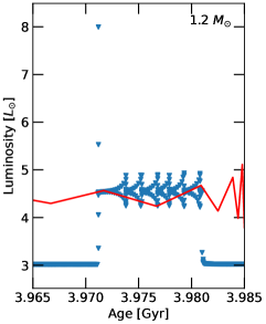
Further insight into the timescales involved can be gained by a detailed look at the 1.32 model undergoing a tidal heating episode that lasts 10 Myr, as illustrated in Fig. 8. The heat is first injected at an age of 3.97 Gyr and causes an immediate, transitory spike in luminosity and surface temperature, but the star then settles onto a new trajectory higher up the HRD with increasing luminosity and decreasing temperature. The first 1 Myr of this trajectory exhibits oscillatory behaviour superimposed on the general trend and by the end of this stage (point 3.9719 in the figure) the surface temperature has returned to its original value but the luminosity is four times higher. For the remainder of the heat-pulse duration, Myr, the star’s luminosity continues to rise and the temperature continues to decrease, until the trajectory intercepts the red-giant branch shortly before the heating switches off (point 3.980). Once the heating is turned off, the star quickly descends the red-giant branch, decreasing in luminosity while its surface temperature remains roughly constant. It takes 8 Myr for the star to return to its original location in the HRD, with the luminosity decreasing from to in the first 1 Myr but taking a further 7 Myr to fall to . At this point the star retakes the original trajectory and the luminosity begins to increase again as the star climbs back up the red-giant branch. The increases (decreases) in the luminosity due to the heat pulse are accompanied by increases (decreases) in the stellar radius.


The appearance of oscillations in the heated 1.2 and 1.26 models merits further comment. The layers into which the heat is injected lie very far from the nuclear processing zone which, for the ages considered, is limited to the central region of the star. They do, however, include the surface convection zone. Kippenhahn diagrams of the models show that the oscillations are present at the base of the convection zone, within the radiative zone (see Fig. 11). These oscillations are forced and for this reason only last the duration of the heat pulse. When heat is added to the outer layers of the model stars, these layers expand and their densities fall. This reduces the opacity in these layers (which correspond to temperatures K, hence the opacities are Kramers-type) and so the radiative region of the star now extends to larger radii. The partially ionized zones of H and He are also lifted to larger radii. Although physical oscillations may occur under such circumstances, we do not model them since our minimum time step is of order 1000 years, far longer than any physical oscillation. The oscillatory behaviour exhibited in Figure 5 is a result of fluctuations in the forcing term due to the mapping between the stellar model and the TIDES model. This affects the base of the heating region, since its position depends on the total radius of the star, and as a consequence all the layers above receive different heat forcing at each timestep, and in particular the base of the convection zone. The behaviour appears oscillatory because the mapped heating at each position diminishes as the stellar radius grows, i.e. the forcing becomes less and this leads to damping. Determining whether true oscillations during a heating pulse can be excited requires a separate investigation which is beyond the scope of this paper.
4 Tidal heating and the isochrone of M67


The old open cluster M67 has an age of around 4 Gyr, which has been determined by a variety of methods including white dwarf cooling (Bellini et al., 2010), isochrone fitting (e.g., Sandquist et al., 2021; Nguyen et al., 2022) and gyrochronology (Barnes et al., 2016). It is used as a case study for stellar evolution codes for testing internal stellar physics such as convective overshooting and diffusion (Choi et al., 2016; Nguyen et al., 2022). In particular, we obtained MIST isochrones for non-rotating models with metallicity from the MIST database555https://waps.cfa.harvard.edu/MIST/ (Choi et al., 2016; Dotter, 2016).
The MIST model , and -band magnitudes were converted to colors by finding the extinction in each passband using the following procedure (Gaia Collaboration, Babusiaux et al., 2018). First, the reddening was obtained from the literature (Taylor, 2007) and was used together with the Cardelli et al. (1989) extinction law to find . The extinction coefficients for each passband, , were found using the formula from Danielski et al. (2018) with the numerical coefficients provided by Gaia Collaboration, Babusiaux et al. (2018). The intrinsic color was then corrected for extinction using
| (5) |
which transforms the MIST model to the M67 color-magnitude diagram. A distance to M 67 of 830 pc, consistent with the range of reported values 800–900 pc (e.g., Geller et al., 2015) was assumed. Figure 9(a) shows a Gaia Data Release 2 (DR2) photometry color-magnitude diagram (CMD) of M 67 designated member stars from Geller et al. (2015) (see also Brady et al., 2023) together with the MIST isochrone for .
We transformed our MESA model outputs to the same CMD by converting the model effective temperature to the Gaia color using the color-temperature relation found by Mucciarelli & Bellazzini (2020). Eq. 5 was then used to correct for extinction. The absolute -band magnitudes were obtained from the model luminosities using the bolometric-correction polynomial fit of Andrae et al. (2018) and then corrected for distance.
Figure 9(b) shows the M 67 stars together with the segments of the evolutionary tracks for the heat-pulse MESA models for the time interval . The heat-pulse models reach regions of the CMD that are blueward of the Main Sequence and above the subgiant branch. These regions contain some M67 designated binary stars. Figure 10(a) shows the partial evolutionary tracks for the heat-pulse models against the MIST isochrone. The evolutionary tracks agree well with the M 67 member stars and with the MIST isochrone. During the heat pulse, the model stars reach regions of the CMD that are slightly bluer and above the main-sequence and subgiant stretches of the isochrone. These models return immediately to their original tracks after the yr pulse. Our highest mass model, , is at the base of the red giant branch when the heat pulse occurs. The pulse lifts it blueward to a new trajectory at higher magnitude, which then tracks towards the red giant branch. Once the pulse is over it descends the red giant branch to its original position. It is possible that mass loss occurs at the highest point but this is beyond the scope of this paper. The effect of the companion on the position of the primary in the CMD is depicted in Fig. 10(b). The companion is a low-luminosity, red star and it has little effect on the model stars, moving them slightly to the red at marginally higher luminosity. The binary systems remain consistent with both the isochrone and the observed M67 designated member stars.
5 Discussion
The tidal heating that was derived for the parameter space chosen for this paper offers an explanation for objects that lie above the sub-giant branch and to the immediate left of the lower red giant branch, as well as for BSSs that lie blueward of the Main Sequence but very close to it. This would mean that these objects are in a very short-lived evolutionary state (0.01 Gyr). Extending the parameter space to more massive companions, closer orbital separations and faster or slower rotation (1.3 or 0.7) would produce higher rates of tidal heating, thus potentially extending the pulse-heated tracks to even bluer locations where the majority of BSS stars lie. A future investigation will explore this possibility.
It is also important to note that within the merger scenario for BSS, the progenitors would necessarily transit through a phase of non-synchronous rotation and be tidally heated. They would therefore appear as BSS’s prior to the merger.
Finally, it is tempting to speculate that oscillations during the pulse-heated phase, if real, could trigger significant mass-loss, stripping the outer stellar layers. Thus, tidal heating is expected to play an important role in all of the BSS formation channels currently under analysis.
Many known binary BSSs are reported to have white dwarf (WD) companions in very long periods. However, this does not exclude the possibility that they are triple systems in which the BSS forms part of an inner system whose binary nature is as yet to be revealed. Other systems do have shorter orbital periods. Vernekar et al. (2023) studied the K2 and TESS data of five BSSs in M67 that are known to be spectroscopic binaries. They estimate an orbital period for WOCS 1007 d, , (similar to what is obtained from isochrones), , 8 (confirming the secondary to be a low-mass WD, which could not have formed through a single-star evolution scenario). Vernekar et al. (2023) postulate that the progenitor system of WOCS 1007 was an almost equal-mass () binary that has experienced mass transfer. WOCS 1007 is known to pulsate but this is due to its location in the Scuti instability region rather than tidally induced perturbations. Although no eclipses were found in the light curves of WOCS 5005 and 1025 (see Fig. 9 for the locations of these systems in the M67 color-magnitude diagram), thereby ruling out high-inclination close binary systems, it does not exclude the possibility of low-inclination close binary companions (Vernekar et al., 2023). No pulsations were found in these systems. The authors report that WOCS 4003 system was more difficult to interpret, with the data suggesting a possible low-inclination compact triple system. Detailed light-curve analysis, such as that carried out by Vernekar et al. (2023), is a powerful technique for constraining the properties of compact binary systems, which is essential for understanding the formation scenarios of BSS.
6 Summary and Conclusions
The HRDs of stellar clusters generally display a small number of stars that are located far from the cluster isochrone. The most striking examples are the Blue Straggler Stars (BSSs) which lie to the blue of the main sequence and tend to have higher luminosities than the main sequence turnoff. These anomalies indicate that the stellar properties have been influenced by physical processes that are not included in the standard structure and evolution models. In this paper we tested the hypothesis that stars with anomalous locations on the HRD are the result of energy that is released as heat in their differentially rotating shearing layers. We obtained the rate of energy dissipation from an ab initio calculation of the tidal perturbations induced by a binary companion and injected it into MESA stellar evolution models to study the star’s response to the injected heat. The surface temperature and luminosity were transformed to the Gaia colors and magnitudes and plotted on the color-magnitude diagram of the old cluster M67, which has a MSTO mass.
We showed that if the dissipated energy is converted into heat, the stellar structure is considerably altered with respect to that of the standard models. In particular, the surface temperature and luminosity are larger, as is the stellar radius. Thus, the star’s location on the HRD is shifted to higher temperatures and luminosities, similar to what is observed in some of the BSSs.
We studied asynchronously rotating stars in the mass range 1.16-1.32 having have a 0.8 companion in a 1.44 d orbit. We found that the heating from the induced differential rotation has the potential to shift the location of stars in the M67 color-magnitude diagram into several anomalous locations, one of which is the blue edge of the main sequence below the turnoff, where it could broaden the main sequence. A second one is the subgiant branch, where it can increase the luminosities of stars above the locus of single-stars, and a third one is the lower giant branch where it can shift stars to hotter temperatures. Stars with different masses, rotation velocities and orbital periods could produce objects in yet other anomalous color-magnitude locations.
Stars that are most likely to undergo heating events are those near the main sequence turnoff, which is when they start expanding and changing their internal rotation structure. Thus, most of the peculiar objects are likely to have masses close to the turnoff mass. However, stars with lower masses (still on the MS) or more evolved stars of higher masses could undergo a tidal heating event if they are severely perturbed by a tidal capture, leading to the formation of a binary system or triple system. The tidal heating mechanism is universal and is expected to apply to stars of all masses.
Models with the largest heating rates develop large amplitude oscillations which are tempting to suggest could drive significant mass-loss. Given the intrinsically asymmetrical properties of tidal heating, such mass-loss during late phases of stellar evolution could give rise to some of the morphologies observed in planetary nebulae.
Finally, we note that our 1.2 pulsed heated model shows a radius increase from 1.50 to 1.75 on a timescale yr. This assumes a constant amount of heat injection but as the radius increases, so does . Thus, the rise during the tidal heating event could be observed on a significantly shorter timescales. Such an event would be interpreted as a relatively slow-rising eruption or outburst, such as observed in some luminous blue variables on the high-mass end of the HRD or Red Novae in the low-mass. Furthermore, because the bloating induced by ultimately comes from the orbital energy, the orbit will shrink. As suggested by Koenigsberger & Moreno (2016), this could lead to a runaway process in which the bloating star absorbs a systematically increasing amount of orbital energy. One possible outcome is the ejection of a shell, allowing the star to contract and stabilize. The alternative would be a merger, in which case the progenitors would transit through a phase of non-synchronous rotation and be tidally heated. They would therefore appear at anomalous HRD locations prior to the merger.
References
- Aerts et al. (2017) Aerts, C., Van Reeth, T., & Tkachenko, A. 2017, ApJ, 847, L7, doi: 10.3847/2041-8213/aa8a62
- Andrae et al. (2018) Andrae, R., Fouesneau, M., Creevey, O., et al. 2018, A&A, 616, A8, doi: 10.1051/0004-6361/201732516
- Barnes et al. (2016) Barnes, S. A., Weingrill, J., Fritzewski, D., Strassmeier, K. G., & Platais, I. 2016, ApJ, 823, 16, doi: 10.3847/0004-637X/823/1/16
- Bellini et al. (2010) Bellini, A., Bedin, L. R., Piotto, G., et al. 2010, A&A, 513, A50, doi: 10.1051/0004-6361/200913721
- Brady et al. (2023) Brady, K. E., Sneden, C., Pilachowski, C. A., et al. 2023, AJ, 166, 154, doi: 10.3847/1538-3881/acf2f3
- Cardelli et al. (1989) Cardelli, J. A., Clayton, G. C., & Mathis, J. S. 1989, ApJ, 345, 245, doi: 10.1086/167900
- Choi et al. (2016) Choi, J., Dotter, A., Conroy, C., et al. 2016, ApJ, 823, 102, doi: 10.3847/0004-637X/823/2/102
- Currie & Browning (2017) Currie, L. K., & Browning, M. K. 2017, ApJ, 845, L17, doi: 10.3847/2041-8213/aa8301
- Danielski et al. (2018) Danielski, C., Babusiaux, C., Ruiz-Dern, L., Sartoretti, P., & Arenou, F. 2018, A&A, 614, A19, doi: 10.1051/0004-6361/201732327
- Dotter (2016) Dotter, A. 2016, ApJS, 222, 8, doi: 10.3847/0067-0049/222/1/8
- Estrella-Trujillo et al. (2023) Estrella-Trujillo, D., Arthur, S. J., Koenigsberger, G., & Moreno, E. 2023, A&A, 670, A44, doi: 10.1051/0004-6361/202244971
- Ferraro et al. (2006) Ferraro, F. R., Sabbi, E., Gratton, R., et al. 2006, ApJ, 647, L53, doi: 10.1086/507327
- Gaia Collaboration, Babusiaux et al. (2018) Gaia Collaboration, Babusiaux, Babusiaux, C., van Leeuwen, F., et al. 2018, A&A, 616, A10, doi: 10.1051/0004-6361/201832843
- Geller et al. (2015) Geller, A. M., Latham, D. W., & Mathieu, R. D. 2015, AJ, 150, 97, doi: 10.1088/0004-6256/150/3/97
- Harrington et al. (2009) Harrington, D., Koenigsberger, G., Moreno, E., & Kuhn, J. 2009, ApJ, 704, 813, doi: 10.1088/0004-637X/704/1/813
- Hills & Day (1976) Hills, J. G., & Day, C. A. 1976, Astrophys. Lett., 17, 87
- Knigge et al. (2009) Knigge, C., Leigh, N., & Sills, A. 2009, Nature, 457, 288, doi: 10.1038/nature07635
- Koenigsberger & Moreno (2016) Koenigsberger, G., & Moreno, E. 2016, Rev. Mexicana Astron. Astrofis., 52, 113
- Koenigsberger et al. (2021) Koenigsberger, G., Moreno, E., & Langer, N. 2021, A&A, 653, A127, doi: 10.1051/0004-6361/202039369
- Landau & Lifshitz (1987) Landau, L. D., & Lifshitz, E. M. 1987, Fluid Mechanics
- Leonard (1989) Leonard, P. J. T. 1989, AJ, 98, 217, doi: 10.1086/115138
- McCrea (1964) McCrea, W. H. 1964, MNRAS, 128, 147, doi: 10.1093/mnras/128.2.147
- McQuarrie (1976) McQuarrie, D. A. 1976, Statistical Mechanics (Harper & Row, New York)
- Melo et al. (2001) Melo, C. H. F., Pasquini, L., & De Medeiros, J. R. 2001, A&A, 375, 851, doi: 10.1051/0004-6361:20010897
- Moreno et al. (2011) Moreno, E., Koenigsberger, G., & Harrington, D. M. 2011, A&A, 528, 48
- Mucciarelli & Bellazzini (2020) Mucciarelli, A., & Bellazzini, M. 2020, Research Notes of the American Astronomical Society, 4, 52, doi: 10.3847/2515-5172/ab8820
- Nguyen et al. (2022) Nguyen, C. T., Costa, G., Girardi, L., et al. 2022, A&A, 665, A126, doi: 10.1051/0004-6361/202244166
- Nine et al. (2020) Nine, A. C., Milliman, K. E., Mathieu, R. D., et al. 2020, AJ, 160, 169, doi: 10.3847/1538-3881/abad3b
- Paxton et al. (2011) Paxton, B., Bildsten, L., Dotter, A., et al. 2011, ApJS, 192, 3, doi: 10.1088/0067-0049/192/1/3
- Paxton et al. (2013) Paxton, B., Cantiello, M., Arras, P., et al. 2013, ApJS, 208, 4, doi: 10.1088/0067-0049/208/1/4
- Paxton et al. (2015) Paxton, B., Marchant, P., Schwab, J., et al. 2015, ApJS, 220, 15, doi: 10.1088/0067-0049/220/1/15
- Paxton et al. (2018) Paxton, B., Schwab, J., Bauer, E. B., et al. 2018, ApJS, 234, 34, doi: 10.3847/1538-4365/aaa5a8
- Paxton et al. (2019) Paxton, B., Smolec, R., Schwab, J., et al. 2019, ApJS, 243, 10, doi: 10.3847/1538-4365/ab2241
- Sandquist et al. (2021) Sandquist, E. L., Latham, D. W., Mathieu, R. D., et al. 2021, AJ, 161, 59, doi: 10.3847/1538-3881/abca8d
- Scharlemann (1981) Scharlemann, E. T. 1981, ApJ, 246, 292, doi: 10.1086/158922
- Taylor (2007) Taylor, B. J. 2007, AJ, 133, 370, doi: 10.1086/509781
- Vernekar et al. (2023) Vernekar, N., Subramaniam, A., Jadhav, V. V., & Bowman, D. M. 2023, MNRAS, 524, 1360, doi: 10.1093/mnras/stad1947
- Zahn (1975) Zahn, J. P. 1975, A&A, 41, 329
Appendix A Energy dissipation rates and Kippenhahn diagrams for selected models
The tidal shear energy dissipation rates in each shell of the 1.2 M⊙ star for the h10 model when it has attained a radius of 1.20, 1.32 and 1.50 are given in Table 4 for a supersynchronously rotating star (=1.1) with a 0.4 companion, and in Table 5 for a subsynchronously rotating star (=0.7) with a 0.8 companion. The ages at which the radii of the latter model are reached, according to the heated MESA model, are listed in Table 3. The radius that is listed in each column is given in and corresponds to the midpoint of the layer. (r) is computed with Eq. (3) and is given in ergs s-1.
Kippenhahn diagrams for the 1.2, 1.26 and 1.32 pulse-heated models The left-hand panels show the stellar interior up to 3.95 Gyr, while the right-hand panels cover the age range between 3.95 and 4.25 Gyr, which includes the period of energy injection into the outer layers. Note that the radius scale is different between the two sets of panels. The blue shaded areas are regions of active nuclear burning, with the shade of blue corresponding to the nuclear energy generation rate, as indicated in the side bar. The inclined lines indicate the regions where convection occurs, while red indicates semi-convection zones. The black line represents the stellar surface.
| 0.42 | 1.68 1029 | 0.52 | 3.09 1029 | 0.57 | 1.69 1029 | 0.65 | 2.65 1029 |
| 0.48 | 2.23 1029 | 0.59 | 4.18 1029 | 0.65 | 3.73 1029 | 0.74 | 4.02 1029 |
| 0.53 | 1.50 1029 | 0.66 | 3.01 1029 | 0.73 | 3.10 1029 | 0.82 | 8.96 1029 |
| 0.59 | 2.78 1029 | 0.73 | 8.11 1029 | 0.81 | 6.72 1029 | 0.92 | 8.69 1029 |
| 0.65 | 6.44 1029 | 0.80 | 1.52 1030 | 0.88 | 2.56 1030 | 1.00 | 4.57 1030 |
| 0.71 | 1.84 1030 | 0.88 | 4.89 1030 | 0.96 | 8.14 1030 | 1.10 | 1.98 1031 |
| 0.77 | 2.55 1030 | 0.95 | 1.18 1031 | 1.04 | 2.67 1031 | 1.19 | 6.56 1031 |
| 0.82 | 1.60 1030 | 1.02 | 1.85 1031 | 1.12 | 4.94 1031 | 1.28 | 1.29 1032 |
| 0.88 | 2.72 1030 | 1.09 | 4.48 1031 | 1.20 | 1.27 1032 | 1.37 | 4.26 1032 |
| 0.94 | 6.47 1030 | 1.16 | 1.96 1031 | 1.28 | 4.79 1031 | 1.46 | 2.34 1032 |
| 0.42 | 1.91 1029 | 0.52 | 4.10 1029 | 0.57 | 2.90 1029 | 0.65 | 7.35 1029 |
| 0.48 | 2.90 1029 | 0.59 | 6.08 1029 | 0.65 | 7.34 1029 | 0.74 | 2.16 1030 |
| 0.53 | 4.77 1029 | 0.66 | 2.24 1030 | 0.73 | 5.48 1030 | 0.82 | 1.90 1031 |
| 0.59 | 2.48 1030 | 0.73 | 2.86 1031 | 0.81 | 6.51 1031 | 0.92 | 1.92 1032 |
| 0.65 | 1.56 1031 | 0.80 | 1.88 1032 | 0.88 | 3.90 1032 | 1.00 | 9.36 1032 |
| 0.71 | 5.62 1031 | 0.88 | 6.26 1032 | 0.96 | 1.18 1033 | 1.10 | 2.52 1033 |
| 0.77 | 1.07 1032 | 0.95 | 1.21 1033 | 1.04 | 2.12 1033 | 1.19 | 4.22 1033 |
| 0.82 | 1.44 1032 | 1.02 | 1.59 1033 | 1.12 | 3.01 1033 | 1.28 | 7.30 1033 |
| 0.88 | 4.27 1032 | 1.09 | 4.42 1033 | 1.20 | 1.09 1034 | 1.37 | 3.93 1034 |
| 0.94 | 3.03 1032 | 1.16 | 1.97 1033 | 1.28 | 6.44 1033 | 1.46 | 2.98 1034 |
