Transition slow-down by Rydberg interaction of neutral atoms and a fast controlled-NOT quantum gate
Abstract
Exploring controllable interactions lies at the heart of quantum science. Neutral Rydberg atoms provide a versatile route toward flexible interactions between single quanta. Previous efforts mainly focused on the excitation annihilation (EA) effect of the Rydberg blockade due to its robustness against interaction fluctuation. We study another effect of the Rydberg blockade, namely, the transition slow-down (TSD). In TSD, a ground-Rydberg cycling in one atom slows down a Rydberg-involved state transition of a nearby atom, which is in contrast to EA that annihilates a presumed state transition. TSD can lead to an accurate controlled-NOT (CNOT) gate with a sub-s duration about by two pulses, where is a negligible transient time to implement a phase change in the pulse and is the Rydberg Rabi frequency. The speedy and accurate TSD-based CNOT makes neutral atoms comparable (superior) to superconducting (ion-trap) systems.
I introduction
There are exciting advances in Rydberg atom quantum science recently Jaksch et al. (2000); Lukin et al. (2001); Saffman et al. (2010); Saffman (2016); Weiss and Saffman (2017); Firstenberg et al. (2016); Adams et al. (2020); Browaeys and Lahaye (2020) because of the feasibility to coherently and rapidly switch on and off the strong dipole-dipole interaction. Such interaction enables simulation of quantum many-body physics Gurian et al. (2012); Tretyakov et al. (2017); De Léséleuc et al. (2019); Schauß et al. (2015); Labuhn et al. (2016); Zeiher et al. (2016, 2017); Bernien et al. (2017); de Léséleuc et al. (2018); Guardado-Sanchez et al. (2018); Kim et al. (2018); Keesling et al. (2019); Ding et al. (2020); Borish et al. (2020), probing and manipulation of single photons Dudin and Kuzmich (2012); Peyronel et al. (2012); Firstenberg et al. (2013); Li et al. (2013); Gorniaczyk et al. (2014); Baur et al. (2014); Tiarks et al. (2014); Li et al. (2016); Busche et al. (2017); Ripka and Pfau (2018); Liang et al. (2018); Li et al. (2019); Thompson et al. (2017), large-scale entanglement generation Ebert et al. (2015); Omran et al. (2019), and quantum computation Ebert et al. (2015); Omran et al. (2019); Wilk et al. (2010); Isenhower et al. (2010); Zhang et al. (2010); Maller et al. (2015); Zeng et al. (2017); Levine et al. (2019); Graham et al. (2019); Madjarov et al. (2020); Jau et al. (2016); Levine et al. (2018); Picken et al. (2019); Tiarks et al. (2019); Jo et al. (2020). To date, however, most effort focused on the effect of excitation annihilation (EA) proposed in Jaksch et al. (2000); Lukin et al. (2001) and reviewed in Saffman et al. (2010); Saffman (2016); Weiss and Saffman (2017); Firstenberg et al. (2016); Adams et al. (2020); Browaeys and Lahaye (2020), although there are other categories as summarized in Table 1. Belonging to the Rydberg blockade regime, EA involves single-atom Rydberg excitation and hence is not sensitive to the fluctuation of interaction. Besides EA, one can also excite both qubits to Rydberg states Jaksch et al. (2000), or explore the antiblockade regime Ates et al. (2007); Amthor et al. (2010), or use the resonant dipole-dipole flip Thompson et al. (2017); De Léséleuc et al. (2019). These latter processes, however, involve two-atom Rydberg excitation and are sensitive to the fluctuation of qubit separation that can substantially reduces the fidelity of a quantum control by using them Jo et al. (2020). It is an open question whether there is another means other than EA to explore the Rydberg blockade regime for efficient and high-fidelity quantum control.
Here, we study an unexplored transition slow-down (TSD) effect of the dipole-dipole interaction between Rydberg atoms. When the state of one atom oscillates back and forth between ground and Rydberg states, its Rydberg interaction does not block a Rydberg-involved state swap in a nearby atom, but slows it down, and the fold of slow-down is adjustable. The resulted TSD denotes the slow-down of the state transfer of one of the two atoms although the collective Rabi frequency is enhanced due to the many-body effect. Albeit appeared as a slow-down, a controlled TSD on the contrary can drastically speed up certain crucial element in a quantum computing circuit, such as the controlled-NOT (CNOT) which is the very important two-qubit entangling gate in the circuit model of quantum computing in both theory Nielsen and Chuang (2000); Williams (2011); Ladd et al. (2010); Shor (1997); Bremner et al. (2002); Shende et al. (2004) and experiment Peruzzo et al. (2014); Debnath et al. (2016). TSD is a new route toward efficient, flexible, and high-fidelity quantum control over neutral atoms because it is implemented in the strong blockade regime which is robust to the fluctuation of interactions.
| Category | Blockade () | Frozen interaction | ||||||
| Feature | Robust to fluctuation of | Sensitive to fluctuation of | ||||||
| Type of |
|
Van der Waals | Dipole-dipole | |||||
| Application | TSD | Excitation annihilation | Phase shift | Antiblockade |
|
|||
| Theoretical proposal | Here | Jaksch et al. (2000); Lukin et al. (2001) | Jaksch et al. (2000) | Ates et al. (2007) | (Intrinsic) | |||
| Realized | CNOT; Toffoli |
|
||||||
| Entanglement |
|
Jo et al. (2020) | ||||||
|
|
|
|
|||||
Though Rydberg atoms have kindled the flame for the ambition to large-scale quantum computing Jaksch et al. (2000); Lukin et al. (2001); Saffman et al. (2010); Saffman (2016); Weiss and Saffman (2017), and recent experiments demonstrated remarkable advances Wilk et al. (2010); Isenhower et al. (2010); Zhang et al. (2010); Maller et al. (2015); Jau et al. (2016); Zeng et al. (2017); Levine et al. (2018); Picken et al. (2019); Levine et al. (2019); Graham et al. (2019); Madjarov et al. (2020); Tiarks et al. (2019); Jo et al. (2020), further progress toward neutral-atom quantum computing is hindered by the difficulty to prepare a fast and accurate CNOT. This is partly because each of those CNOT gates was realized via combining an EA-based controlled-Z () and a series of single-qubit gates Isenhower et al. (2010); Zhang et al. (2010); Maller et al. (2015); Zeng et al. (2017); Graham et al. (2019); Levine et al. (2019), leading to CNOT durations dominated by single-qubit operations (e.g., over s in Levine et al. (2019); Graham et al. (2019)). In contrast, an TSD-based CNOT has a duration about by only two Rydberg pulses, i,e., needs no single-qubit rotations, where is a transient moment to implement a phase change in the pulses and the Rydberg Rabi frequency. Using values of and from Graham et al. (2019); Levine et al. (2019), the TSD-based CNOT (duration s) would be orders of magnitude faster than those in Graham et al. (2019); Levine et al. (2019), which means that a neutral-atom CNOT can be much faster than the CNOT (or ground Bell-state gate) by trapped ions Cirac and Zoller (1995); Sørensen and Mølmer (1999); Ballance et al. (2015, 2016); Gaebler et al. (2016) (notice that the fast ion-trap gates in Schäfer et al. (2018); Zhang et al. (2020) are phase gates). Although still inferior to superconducting circuits You and Nori (2005); Devoret and Schoelkopf (2013) where CNOT gate times can be around ns Barends et al. (2014), the TSD-based CNOT is applicable in scalable neutral-atom platforms that are ideal for long-lived storage of quantum information in room temperatures.
II A two-state case
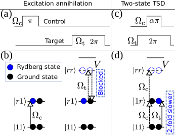
The simplest model of TSD consists of two nearby atoms, each pumped by a laser pulse that induces a transition between a ground state and a Rydberg state . The Rabi frequency is for the control (target) qubit, and the dipole-dipole interaction in is assumed large compared to so that is not populated. For Rydberg interaction of the van der Waals type, is limited because in this regime the native dipole-dipole interaction should be much smaller than the energy gaps between nearby two-atom Rydberg states Walker and Saffman (2008), and thus the qubit spacing should be large enough. On the other hand, a direct dipole-dipole interaction can be huge for high-lying Rydberg states although it is no longer a pure energy shift. In this sense, the residual blockade error of the order Saffman and Walker (2005) can be negligible in the strong dipole-dipole interaction regime as long as the two-atom spacing is beyond the LeRoy radius.
Figure 1 shows a contrast between EA and a two-state TSD, where the pulse sent to the control atom is applied during , and that to the target atom is during with . Starting from an initial two-atom state , the wavefunction at becomes
| (1) |
During , the system Hamiltonian is
| (2) |
where includes excitation between and and the dipole-dipole flip from . Focusing on the strong interaction regime, can be discarded because is not coupled Jaksch et al. (2000) and hence , where and . When , we have , so that the wavefunction at , given by , is equal to Eq. (1), and it is like that nothing happens to the target qubit upon the completion of the drive in the control qubit. Then, because the pulse for the control qubit ends at , the continuous pumping on the target qubit drives the state to at , i.e., a pulse, instead of a pulse, completes the transition , which corresponds to a 2-fold slow-down.
III A fast CNOT
To show the strength of TSD in quantum information, we would like to consider TSD in three states. This is because the two-state TSD ends up in a Rydberg state which is not stable, while quantum information shall be encoded with two qubit states and in the more stable ground manifold. For frequently used rubidium and cesium atoms, and can be chosen from the two hyperfine-split ground levels with a frequency difference of several gigahertz.
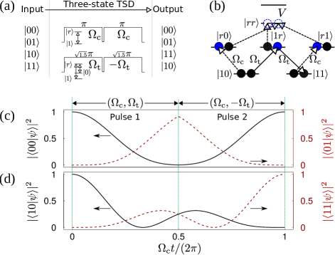
Consider a ground-Rydberg-ground transition chain , i.e., a state swap between the two long-lived qubit states via a metastable Rydberg state . The three-state TSD is implemented by pumping the control and target qubits with respective Rabi frequencies and for the same duration, with transition for the control qubit and for the target qubit. This requires a setup capable of pumping both qubit states to a common Rydberg state in the target qubit, which is feasible as experimentally demonstrated for two-atom entanglement about a decade ago Wilk et al. (2010) and for -state preparation in atom ensembles later Ebert et al. (2015). Because is not pumped in the control qubit, the Hamiltonian is H.c. for the input states and , where the subscript () denotes that the Hamiltonian applies when the input state for the control qubit is . For the remaining input states, we consider the ordered basis for the following Hamiltonian
| (8) |
where we ignore the two-atom Rydberg state with reasons shown below Eq. (2). By diagonalizing Eq. (8) one has
| (9) |
where with are four eigenvectors of Eq. (8), with eigenvalues , respectively [the fifth eigenvector does not enter Eq. (9)], where and
| (10) | |||||
We proceed to describe an accurate and exceedingly fast CNOT by a spin-echo assisted TSD. The sequence consists of two pulses, each with duration and condition , shown in Fig. 2(a). A phase change (requiring a time ) is inserted between the pulses sent to the target qubit so as to induce spin echo, where can be around ns Levine et al. (2019). The spin echo suppresses the state swap of the target qubit if the control qubit is initialized in Shi (2018a, 2020a); but when the control qubit is initialized in , it is pumped to which results in TSD in the target qubit, i.e., the transition in the target qubit, which can occur with a pulse duration if no TSD is used Shi (2018b), will be slowed down by a fold of . The mechanism is understood in two steps. First, during with , the input state or evolves according to , and after a phase change to the Rydberg Rabi frequency which may require a finite transient time , the state evolution becomes during the second pulse, leading to at the end of the sequence. Second, according to Eq. (10), the first pulse during evolves the input state according to
| (11) |
which becomes
| (12) |
at because . In Eq. (12), the eigenvectors , , are defined in Eq. (10) with Rabi frequencies during . During , the Hamiltonian has Rabi frequencies with the eigenvectors the same as in Eq. (10), but the expressions for become
Using Eqs. (10) and (LABEL:eq08) we cast Eq. (12) into
| (14) |
i.e., the state at is like if Rabi frequencies were used during the first pulse. Equation (14) is the key feature enabling a fast CNOT. After the second pulse, the state at becomes that can be rewritten as thanks to Eq. (14), which further reduces to according to Eqs. (9) and (11). A similar analysis shows that if the initial state is , it maps to upon the completion of the pulse. So the following map is realized
| (15) |
which is the standard CNOT. A numerical simulation of the population evolution by and in Eq. (8) is shown in Figs. 2(c) and 2(d) for the input states and , respectively, where the transient time is ignored for brevity.
High fidelity is possible with the TSD-based CNOT. To estimate the intrinsic fidelity limited by Rydberg-state decay and Doppler dephasing, we consider atomic levels and Rydberg laser Rabi frequencies in recent experiments Graham et al. (2019); Levine et al. (2019), and numerically found that the fidelity of the TSD-based CNOT or Bell state would reach () with experimentally affordable effective temperatures K of qubit motion Picken et al. (2019); Zeng et al. (2017); Graham et al. (2019). As detailed in Appendix A.2, this estimate assumes that the field for and that for in the target qubit copropagate, leading to opposite phases in the two transitions of the chain , where is the wavevector and the speed of the target qubit along the propagation direction of light. Then, the state transfer from to (or the reverse) picks up two opposite phases which partly suppresses the dephasing. Fortunately, our method is not strictly dependent on the above dephasing-resilient configuration. For example, for the worst case of counterpropagating fields so that the sequential state transfer from to picks up a total phase , simulation in Appendix A shows that fidelity over is achievable for K in room temperatures. The robustness against the Doppler dephasing benefits from the avoidance of shelving the control atom on the Rydberg level in free flight during pumping the target atom as required in an EA-based CNOT Müller et al. (2009); Shi (2018b).
The above analysis assumes MHz corresponding to an interatomic distance m. When MHz with larger m (where crosstalk can be negligible Graham et al. (2019)), the fidelity would be () with K in room temperatures (see Appendix B for details). This benefits from that our CNOT is not sensitive to the change of interaction in the strong blockade regime. Finally, with fluctuation (of relative Gaussian width ) of the two Rabi frequencies for the two transitions in the target qubit, very small extra error arises for as detailed in Appendix C. So, high fidelity is achievable since the power fluctuation of Rydberg lasers can be well suppressed Levine et al. (2018, 2019).
IV Discussion and conclusions
The CNOT in Eq. (15) is implemented within a short time plus a transient moment for a phase change between the two pulses, where can be negligible as in Levine et al. (2019). Although a phase twist is used in both Levine et al. (2019) and here, our TSD method is drastically different in physics from the method of Levine et al. (2019) as discussed in Appendix D. Note that Eq. (15) does not depend on any single-qubit gates if one starts from Eq. (8). If or -orbital Rydberg states are used, two-photon transitions can be applied which leads to ac Stark shifts for the ground and Rydberg states. As shown in Appendix E, these shifts are annulled in Eq. (8) which is achievable by choosing appropriate ratio between the detuning at the intermediate state and the magnitudes of the fields for the lower and upper transitions Maller et al. (2015).
Our CNOT gate duration can be s with Rydberg Rabi frequencies ( MHz) like those realized in Graham et al. (2019); Levine et al. (2019) that showed CNOT gate durations orders of magnitude longer than here. Previous CNOT gates Zhang et al. (2010); Maller et al. (2015); Zeng et al. (2017); Graham et al. (2019); Levine et al. (2019); Isenhower et al. (2010) required two or more single-qubit rotations to convert to CNOT, which was usually achieved with two-frequency Raman light Isenhower et al. (2010); Zhang et al. (2010); Zeng et al. (2017); Levine et al. (2019), or with microwave driving assisted by Stark shift of laser fields Graham et al. (2019); Maller et al. (2015). High-fidelity realizations of such gates came with long gate durations Xia et al. (2015); Wang et al. (2016); Graham et al. (2019); Levine et al. (2019), although they can also be carried out rapidly in proof-of-principle experiments Yavuz et al. (2006); Jones et al. (2007) where high fidelity is not concerned. The atom traps have finite lifetimes Saffman (2016) and a faster protocol can lead to more CNOT cycles before the qubit arrays should be reloaded. Because a practical quantum processor tackling real problems uses a series of quantum gates including CNOT Nielsen and Chuang (2000); Williams (2011); Ladd et al. (2010); Shor (1997); Bremner et al. (2002); Shende et al. (2004); Peruzzo et al. (2014); Debnath et al. (2016), certain computation tasks can be executed only with fast enough CNOT in each cycle of laser cooling and loading of atom array. The studied speedup of the minimal functional quantum circuit shows a possibility to confront the problems of finite lifetime of atom traps which limits the capability of a neutral-atom quantum processor. Moreover, concerning the ratio between the coherence time and the CNOT gate time, the TSD method makes neutral-atom systems competitive with superconducting and ion-trap systems as compared in detail in Appendix F.
In conclusion, we have explored another effect of Rydberg blockade by dipole-dipole interaction in neutral atoms, namely, the effect of transition slow-down (TSD). We show that TSD can speed up a neutral-atom quantum computer by proposing an exceedingly fast TSD-based CNOT realized by two pulses separated by a short transient moment for changing the phase of the pulse. The exotic TSD is an excellent character of dipole-dipole interactions other than the well-known excitation annihilation effect that can push Rydberg-atom quantum science to another level.
ACKNOWLEDGMENTS
The author thanks Yan Lu for useful discussions. This work is supported by the National Natural Science Foundation of China under Grant No. 11805146 and Natural Science Basic Research plan in Shaanxi Province of China under Grant No. 2020JM-189.
Appendix A Gate fidelity
Before analyzing the gate error, we would like to emphasize that TSD is particularly useful for speeding up the minimal functional quantum circuit, namely, the CNOT. The CNOT protocols by EA in previous methods involve multiple switchings of the external control fields which brings extra complexity to the experimental implementation, elongate the gate duration, and introduces extra errors from the fluctuation of the control fields and from the intrinsic atomic Doppler broadening. Previous effort for suppressing these errors includes a gate based on quantum interference Shi (2019); Levine et al. (2019), but going from to the more useful CNOT (or to create Bell states in the ground-state manifold) still needs several single-qubit operations Graham et al. (2019); Levine et al. (2019); Isenhower et al. (2010); Zhang et al. (2010); Maller et al. (2015); Zeng et al. (2017). For example, the first experimental neutral-atom CNOT needed five or seven pulses Isenhower et al. (2010), and the recent CNOT in Levine et al. (2019) used two (four) pulses in the control (target) qubit besides several short pulses for phase compensation. The central procedure of the CNOT in Levine et al. (2019) is via combining (i) a two-qubit -like gate by two pulses of duration about with a phase change inserted between the pulses that requires an extra transient time , (ii) a short pulse to compensate an intrinsic phase to recover a from the -like gate, and (iii) two single-qubit rotations of duration (s therein) in the target qubit, where is the Rydberg laser Rabi frequency and is the hyperfine laser Rabi frequency between the two qubit states. Page 4 of Ref. Levine et al. (2019) indicates that the -like gate needs s, and it had MHz (see page 1 and 2 of Levine et al. (2019)), thus s ns; we assume such a fast phase change time here. Figure 3(d) of Ref. Levine et al. (2019) presents a CNOT sequence with durations equal to those of two , one , and the -like, i.e., , and thus the CNOT sequence needs about s therein (the actual gate durations should be larger when accounting for gaps between pulses therein). In contrast, the TSD-based CNOT needs a duration about which is only s with MHz from Ref. Graham et al. (2019) (Ref. Levine et al. (2019)).
One may image that if the single-qubit rotations in Refs. Graham et al. (2019); Levine et al. (2019) are implemented by the transition chain , then their gate durations can also be small. But there will be problems in this assumption. This is because the single-qubit rotations necessary to transform to CNOT are two gates that transfer to (see Fig. 5(a) of Graham et al. (2019) or Fig. 3(d) of Levine et al. (2019)). But the pumping by H.c can not achieve this since one can easily prove that starting from , the populations in will be , where . This means that there is no way to use the resonant transition chain for the rotation. On the other hand, one may also imagine a succession of a pulse on , a pulse on , and a pulse on can, e.g., realize a rotation. However, the extra time to shelve an atom in Rydberg state leads to extra Doppler dephasing, and the frequent turning on and off of Rydberg lasers can lead to extra atom loss Maller et al. (2015).
Below, we analyze gate imperfections due to the prevailing intrinsic Rydberg-state decay and Doppler broadening. These are the dominant intrinsic errors in gate operations Graham et al. (2019) while technical issues such as laser noise is in principle not fundamental. From here to Appendix C, we take, as an example, 87Rb qubits and consider the intermediate level for Rydberg pumping, where the two detunings at should be different for the two transitions and . For an -orbital rubidium Rydberg state with principal quantum number around , the lifetime of is about s at a temperature of K by the estimate in Beterov et al. (2009). When the lower and upper fields counterpropagate along, e.g., , the wavevector is nm-1 Shi (2020b). We assume that the two qubits are initially located at the centers of the traps at and respectively. The traps are usually turned off during Rydberg pumping, and the free flight of the qubits leads to time-dependent Rabi frequencies for the control qubit, and for the two transitions in the target qubit, where are the projection of velocity along for the control and target qubits, respectively. With a finite atomic temperature , there is a finite distribution for the speeds , where is a Gaussian Graham et al. (2019); Shi (2020b).
A.1 Rydberg-state decay
Although the gate duration, when neglecting the transient time ( ns as shown above) for phase change in the pulses, is , the main decay error arises when the atoms are in Rydberg state Saffman and Walker (2005) supposing the intermediate state is largely detuned. By using the estimate in Zhang et al. (2012), the decay error of the TSD-based CNOT gate can be approximated as
| (16) | |||||
which is by numerical simulation. Consider a set of experimentally feasible Graham et al. (2019) values of Rydberg Rabi frequencies MHz, we have for qubits in an environment temperature of K. Alternatively, a more detailed numerical simulation by using the optical Bloch equation in the Lindblad form with correct branching ratios Shi (2019) can predict a slightly lower because some population can decay to qubit states that will again contribute to the gate operation.
A.2 Doppler dephasing
For the TSD-based CNOT to be resilient to Doppler dephasing, the two fields for the lower transitions and shall copropagate along , and those for their upper transitions shall copropagate along , so that the wavevectors for have (approximately) the same value . Here is symbolic for the intermediate state and one shall bare in mind that the detunings at for the two transition chains must have a large difference; alternatively one can use different fine states in the manifold for the two transition chains (the numerical results in Tables 2 and 3 stay similar). Then, the transition becomes
| (17) |
when accounting for the atom drift. The above transition mainly transfers the population between the two hyperfine states, which means that if negligible population stays at , the two phases and add up for any moment, leading to negligible phase noise because for the population transfer from to . However, this is not ideal since there is always some population at during the process. Nonetheless, that there is partial phase cancellation can suppress the Doppler dephasing compared to usual cases.
For the control qubit, the transition still has the usual Doppler dephasing. However, the pumping in the control is immersed in the TSD and does not put much population in the Rydberg state. Numerical simulation shows for either or in each gate sequence.
To show the robustness of the TSD-based CNOT against the Doppler dephasing, we numerically simulate the state evolution by using H.c. for the input states and , and
| (24) |
for the input states and , where Eq. (24) is written with the basis , where represents the interaction of the state . Because of the Doppler dephasing, the gate map in the basis changes from the ideal form
| (29) |
to
| (34) |
where , and can be calculated by sequentially using and for the input states and , while , and can be calculated using, sequentially, and , for the input states and . To study the robustness to Doppler dephasing, we would like to see errors mainly from the Doppler dephasing if the blockade error is negligible. So we adopt a large blockade interaction MHz as in Ref. Saffman et al. (2020). We choose MHz, define the rotation error by Pedersen et al. (2007)
| (35) |
and evaluate the ensemble average with
| (36) |
where the sum is over sets of speeds , where applies values equally distributed from to m/s because the atomic speed has little chance to be over m/s for the temperatures K considered in this work. The approximation by Eq. (36) has little difference from a rigorous integration. More details can be found in Shi (2020b) for the method of numerical simulation.
Case 1.–By using (for ) and (for ) for the first pulse, and and for the second pulse, the ensemble-averaged rotation errors are given in the second row of Table 2, with effective atomic temperatures above K which was achievable in experiments Picken et al. (2019). From these results, one can see that the CNOT fidelity can reach with qubits cooled to around K in a K environment.
Case 2.–To further suppress the Doppler dephasing, we consider switching propagation directions of fields for the control qubit between the two pulses. In other words, the Hamiltonians (for ) are and for the first and second pulses, respectively. The ensemble-averaged rotation errors are shown in the third row of Table 2. From the results in Table 2, one can see that the CNOT fidelity has a slight improvement if this latter case of configuration is employed. The mechanism for the extra suppression of Doppler dephasing in this latter case lies in that the population going, e.g., from to , obtains some phase error due to the action and ; subsequently, the second pulse pumps to and induces some phase error due to the action and , which means that the phase terms between the two pulses are continuous which is better for the desired transition to occur. For case 1, the pumping from to has a phase term at the end of pulse 1, which becomes when the population begins to go back at the start of pulse 2, i.e., there is a phase jump. More details about the influence on gate fidelity from atom-drift-induced phase change in Rabi frequencies can be found in Shi (2020b). Since this latter case is a little involved and the increase of fidelity is marginal, it is only of interest in the future when technical issues are resolved so that a fidelity level beyond is technically achievable.
| K) | 5 | 10 | 15 | 20 | 50 | |
|---|---|---|---|---|---|---|
| Case 1 | ||||||
| Case 2 |
| K) | 5 | 10 | 15 | 20 | 50 | |
|---|---|---|---|---|---|---|
| Case 1 | ||||||
| Case 2 |
The result in Table 2 accounts for both the population errors and the phase errors. In experiments, usually the phase errors are not important especially in the characterization of the Bell state Levine et al. (2019); Graham et al. (2019). Thus we continue to study the strength of TSD-based CNOT for achieving high-fidelity Bell states.
A.3 High-fidelity Bell states
A TSD-based CNOT can map the initial product state to the Bell state without resorting to extra single-qubit gates (except the state initialization). The Rydberg superposition time is equal to that in Sec. A.1. We follow Ref. Levine et al. (2019) by evaluating the infidelity as , where with evolved by using the pulse sequence as in Sec. A.2 for the input state . The numerical results are given in Table 3, which shows that in room temperatures, the Bell state can be created with a fidelity if qubits are cooled to the level of K, which is affordable according to the atom cooling achieved in previous experiments Picken et al. (2019); Zeng et al. (2017).
Finally, we would like to emphasize that it is not so crucial to have the Doppler-resilient configuration (with copropagating fields) for the two transition chains in the target qubit, as discussed around Eq. (17). Consider the worst case with largest dephasing, i.e., if the two sets of fields counterpropagate so that Eq. (17) becomes , then the motional dephasing error should be larger. For example, we numerically found that the Bell-state errors in the second row (case 1) of Table 3 become for K; similar results can be found for the TSD-based CNOT. With for qubits in an environment of K, the Bell-state fidelity would be at K. This still large fidelity means that for experimental convenience, high fidelity is possible with any configuration for the propagation directions for the two sets of fields if errors other than the intrinsic Doppler dephasing and Rydberg-state decay can be avoided.
Appendix B Interatomic distances
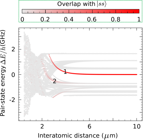
The dipole-dipole interaction is a function of interatomic distance . For to be large enough so that the blockade error is negligible, should be small enough. In order to avoid wavefunction overlap, the distance between the nuclei of the two Rydberg atoms shall be larger than the Le Roy distance which can be calculated by using the open source library of Ref. Šibalić et al. (2017). For the parameters chosen as an example in this work, the Le Roy distance is m for two rubidium atoms in the state , and we can consider longer interatomic distance in the range of m. The dipole-dipole interaction will couple the two-atom state to many other states. To find the interaction, we consider states coupled from the initial states ( and denote the principal and angular momentum quantum numbers, respectively), with , and (because states couple to states, which couple to -orbital and to -orbital states, and so on), and consider energy gaps between pair states within GHz. After diagonalization, the energy map is shown in Fig. 3. In Fig. 3, the color denotes the population of the state in the diagonalized state; the color can also be understood as how possible if one atom is already in the state , what will the chance be to populate the state if the other atom is Rydberg pumped via, e.g., the intermediate state.
For the TSD to hold, we focus on the strong blockade regime where the two-atom Rydberg state shown in Fig. 3 is barely populated. In this case, the smallest energy of the diagonalized eigenstate matters, or more accurately, the state with the smallest eigenenergy that can be coupled (marked by red) plays the role. In Fig. 3, one can find that for m, there are mainly three eigenstates, one with a positive energy (labeled as state 1), and the other two with negative energy. For those two that have negative energy, the one we focus on is the state with more overlap with , whose energy is sometimes lower and sometimes higher than the energy of the other with less population in . The two states we focus on are labeled by 1 and 2 in Fig. 3. State 1 has the largest component in : at m, the amplitude overlap between state 1 and is . For state 2, its overlap with is when m and is negligible when is beyond m. The eigenenergy of these two states are listed in Table 4, from which one can see that around m, the interaction can be represented by the eigenenergy of state 2, which is largest for the cases shown in Table 4.
| m) | 2.6 | 3.0 | 3.6 | 4.0 | 4.6 | |
|---|---|---|---|---|---|---|
| State 1 | (MHz) | 1600 | 780 | 340 | 180 | 94 |
| State 2 | (MHz) | -280 | -510 | -590 | -650 | -670 |
| (MHz) | K) | 5 | 10 | 15 | 20 | 50 |
|---|---|---|---|---|---|---|
| 50 | ||||||
| 100 | ||||||
| 200 | ||||||
| 300 | ||||||
| 400 |
To have MHz, the above study shows that placing the two qubits with a distance around m seems necessary. With such a distance, the analysis in Ref. Graham et al. (2019) shows that the crosstalk error is about if the waist ( intensity radii) of the laser beams is m. To reduce the crosstalk, it is possible to use super-Gaussian Rydberg beams, as detailed in Ref. Gillen-Christandl et al. (2016). Another possibility is to use higher Rydberg states so that the dipole-dipole interaction can be as large as MHz at a larger interatomic distance, and hence the laser-beam crosstalk can be avoided.
If only commonly used Gaussian Rydberg beams are employed for a Rydberg state of principal quantum number around , then smaller values of can be used for larger interatomic distances so as to avoid crosstalk. For the values MHz, the fidelity of our gate is shown in Table 5, which shows that with MHz, the rotation error is about with K, and the interatomic distance should be around m where crosstalk can be ignored safely () if the waists for the lower and upper lasers are both m. Taking into account the decay error, this means that our gate would have a fidelity with K in room temperatures.
Appendix C Amplitude fluctuation of laser fields
Our TSD-based CNOT requires the Rabi frequencies for the two transitions to be equal in the target qubit. Here we investigate the impact on the gate fidelity if this condition is not satisfied.
We assume that the Rabi frequency obeys a Gaussian distribution
| (37) |
around the desired value , where t1, t2 denotes the two channels and . By using the Gaussian distributed Rabi frequencies in the target qubit, one can evaluate the averaged fidelity by
| (38) |
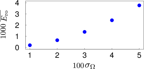
where is evaluated by using the gate fidelity with and for the two transitions and . In Eq. (38), the integration is approximated by the sum over 121 sets of , each of which applies values . With , the result is shown in Fig. 4. One can see that with quite large relative fluctuation of Gaussian width , the fidelity is still larger than . There is little relation between the Doppler dephasing and fluctuation of Rabi frequency, and one can expect that the gate fidelity can be evaluated by combining Table 2 and Fig. 4 if the fluctuation of the Rabi frequencies is not quenched.
In Ref. Levine et al. (2018), the power fluctuation of the Rydberg lasers was suppressed below for preparing ground-Rydberg entanglement, which means that the Rydberg Rabi frequencies were suppressed to have relative noise below in Ref. Levine et al. (2018). More than one year later, in Ref. Levine et al. (2019), preparation of high-fidelity ground-state entanglement was reported by the same group, which was a significant progress. We suppose that the laser noise was even more suppressed in Ref. Levine et al. (2019) compared to the earlier experiment in Ref. Levine et al. (2018), and thus we consider the relative Gaussian width of the fluctuation up to .
Appendix D Comparison with other fast Rydberg gates
It is useful to compare our CNOT with other fast entangling methods with Rydberg atoms. The comparison focuses on physical mechanism and their application in quantum computing.
A popular method to generate entanglement by Rydberg interactions is to use the EA mechanism Jaksch et al. (2000). The standard way to use it is a three-pulse sequence for a gate in the form of
| (43) |
in the basis , where the blockade takes effect in the state . To use it for quantum computing in the circuit model, the gate in Eq. (43) needs single-qubit gates to become a CNOT. By this method, a most recent experiment in Ref. Graham et al. (2019) realized a CNOT of duration more than 100 s with Rydberg Rabi frequencies MHz because of the slow single-qubit gates. Physically, this method depends on a missed phase accumulation in an annihilated Rabi cycle for the input state by the Rydberg blockade.
The other recent experiment in Ref. Levine et al. (2019) used detuned Rabi cycles for entanglement combined with detunings found by optimal control. The method is essentially identical to the interference method proposed in Ref. Shi (2019), as can be easily verified by looking at the similar structure of the gate matrix [with the same basis as in Eq. (43)]
| (48) |
in Refs. Levine et al. (2019); Shi (2019) (Ref. Shi (2019) proposed two gates among which the first is quoted here). Compared to the initial interference method, Ref. Levine et al. (2019) used optimal-control-found parameters and phase twist in the Rydberg pumping within the blockade regime so as to realize (and thus the gate in Ref. Levine et al. (2019) can be called a -like gate). Because of the detuned Rabi cycles used, there is no way to realize a gate with , where is an integer with . To use it in quantum computing, several single-qubit gates must be used to transform the gate in Ref. Levine et al. (2019) to the CNOT so their final CNOT duration was more than s with Rydberg Rabi frequencies MHz. Without using the detuned Rabi cycles, the method in Ref. Levine et al. (2019) can not work. The physical mechanism of Ref. Levine et al. (2019) is that dynamical phases in detuned Rabi cycles are accumulated.
In order to compare with the gates in Eqs. (43) and (48) which have a diagonal form, the TSD-based CNOT in the basis of can be rewritten as
| (53) |
with the basis , where . The CNOT duration would be less than s with Rydberg Rabi frequencies MHz by the TSD method. The blockade interaction is in and the pumping on the target qubit induces a transition from to with a Rabi frequency while further excitation to is blocked. Each of the two pulses in the TSD-based CNOT sequence induces a complete rotation which leads to a phase change to . The change of the sign of between the two pulses does not change this picture, and thus a total phase is accumulated in . Since , acquires no phase term in practice. On the other hand, the input state only experiences two pulses (i.e., a pulse) in the control qubit which results in a phase change to it. The pumping of the target qubit experiences spin echo for the input state , thus no phase appears for it. So, the physical mechanism of the gate in Eq. (53) is fundamentally different from those in Eqs. (43) and (48); in fact, the drastically different forms of the three gate maps reveal this. To sum up in one word, Eq. (43) relies on a missed phase change in an annihilated Rabi cycle, Eq. (48) relies on three phase changes in three detuned Rabi cycles, and (53) relies on a phase change in a resonant Rabi cycle. For quantum computing, the gate in Eq. (53) is exactly a CNOT in the basis of , and thus is more useful compared to Eqs. (43) and (48).
Because a phase twist is used in realizing both Eq. (48) and Eq. (53), one may guess that they are similar. But the following facts show their distinct physics: (i) detuned Rydberg pumping is used in Eq. (48), but resonant Rydberg pumping is used in Eq. (53); (ii) three input states acquire phase terms in Eq. (48), but only one input state acquires a phase term in Eq. (53); (iii) the population in Rydberg state can reach 1 for the fourth input state in Eq. (53), while there is no way to realize such an effect in Eq. (48). This last effect basically means that the mechanism for realizing Eq. (53) can be used to realize a high-fidelity multi-qubit gate: one can use TSD to excite the input state to which can block the Rydberg pumping in a nearby atom (of course care shall be taken for the design of such a gate); notice that the three-qubit gate in Ref. Levine et al. (2019) requires exciting the two edge atoms to block the Rydberg pumping in the middle atom which results in error due to the residual blockade between the two edge atoms. For the method in Eq. (48), detuned Rabi cycles are used and it can not excite one Rydberg excitation in the blocked excitation [for the input state in Eq. (48)] , and thus it is not possible to extend the method in Eq. (48) to a high-fidelity multi-qubit gate. This means that the underlying physics in Eq. (53) is different from that of Eq. (48).
Note that the basis transform used to write the TSD-based CNOT in Eq. (48) is used only for clarifying the physics, but not for practical use since in a large-scale quantum computer the way to encode quantum information shall be based on a commonly used qubit basis in all registers (otherwise the information loading and retrieving will face trouble). For example, to initialize the atomic arrays, the quantization axis is fixed by applying, e.g., an external magnetic field, and the qubit states and are chosen from two hyperfine levels with different energy. So, the states are no longer eigenstates because of the applied external fields, and new state detection schemes shall be designed. In a large-scale quantum computer, to play the role of control or target is not fixed for any qubit: a computation task is divided into a series of unitary operations, in different unitary operations, the same qubit sometimes serves as a control, and sometimes as a target. This means that if one uses a hybrid coding with for the control and for the target, an exceedingly large amount of transforming operations between and should be used in the quantum circuit. So, it is impractical to use for information coding in the control, and to use for information coding in the target; for a proof-of-principle study either in theory or in experiment, it may be of interest, but not for a realistic large-scale quantum computer.
Appendix E AC Stark shifts
There is a detailed study about the ac Stark shifts in a two-photon Rydberg excitation in Ref. Maller et al. (2015). Appendix B of Maller et al. (2015) presents a detailed calculation of the ac Stark shifts accounting for the hyperfine splitting of the intermediate state, where one can find that compensation of the ac Stark shifts is feasible. Below, we ignore the hyperfine splitting of the intermediate state to give a brief introduction. More details can be found in Ref. Maller et al. (2015).
Here, we choose the qubit states by and of cesium. The state is driven to (in the manifold) with laser fields that are left-hand circularly polarized (note that this is a little different from Ref. Maller et al. (2015)), which is further excited to . The Hamiltonian for a two-photon Rydberg excitation is (in this section we explicitly put in Hamiltonians)
| (54) | |||||
where is defined as the frequency of the laser field deducted by the frequency of the atomic transition. Note that we have not included the nonresonant shift in the equation above. When is very large compared to the decay rate of , the intermediate state can be adiabatically eliminated, leading to
| (55) | |||||
where , and according to Ref. Maller et al. (2015) the effective detuning at the level is
| (56) | |||||
where is the elementary charge, the mass of the electron, and and are the frequency and electric field amplitude of the laser field, where and for the lower and upper transitions, respectively. Similarly, for the ground state, the effective detuning is
| (57) | |||||
where and are the nonresonant polarizabilities from the lower and upper fields that can be calculated via the sum over transitions to other states except the intermediate state . Meanwhile, there is a shift on the ground state
| (58) | |||||
where is the frequency separation between and , and is a factor determined by the selection rules. Because and is negative, the off-resonant shift will be negative, and thus it is necessary for the resonant shift to be positive. So, both in Eq. (57) and in (58) shall be positive, which further means that shall be larger than 1.
For the case when is much larger than the hyperfine splitting of the intermediate state, we ignore its hyperfine splitting and then it can be written as . When right-hand polarized fields are used for coupling qubit states and the states, the square of the ratio of the coupling between and and that between and is
| (59) |
which is 8. To shift to zero, one can simply adjust the frequency of the laser fields for addressing the upper transition. To compensate the Stark shifts at and , Eqs. (57) and (58) indicates that , which means that we shall choose GHz (for rubidium it would be GHz) which is near to values used in experiments Isenhower et al. (2010); Maller et al. (2015). With satisfied, an appropriate set of satisfying Eq. (57) would satisfy Eq. (58), too. With the given data for the radial coupling between ground and states and the values of (page 6 of Maller et al. (2015)), Eq. (57) reduces to , where , which can be used to set up the ratio .
We have shown the method to compensate the Stark shifts if pumping applies only to the transition . For the target qubit, there will be another transition required, . Then, four fields lead to Stark shifts in the two qubit states (two equations), and there is a condition that the Rabi frequencies for shall be equal (a third equation). Moreover, there will be two detunings at the intermediate states for these two transitions. Altogether there are three equations for six variables and hence the problem is solvable. The Stark shift at can be compensated by adjusting the central frequencies of the laser fields. So, Eq. (24), or Eq. (3) in the main text, can be realized.
For one-photon excitation of -orbital Rydberg states, the off-resonant ac Stark shift on or from the resonant field is positive, but one can use another field of larger wavelength to induce a negative shift. Then, a similar set of equations like Eqs. (57) and (58) can be established to compensate the Stark shifts. For the shift on the Rydberg state, one can shift the wavelength of the laser field to recover the resonance condition for .
Appendix F CNOT in other systems
It is useful to compare the speed of CNOT in different physical systems by using the ratio , where is the coherence time (pure spin dephasing or the inhomogeneously broadened ), and is the duration of CNOT. First, for neutral atom qubit systems, in Ref. Wang et al. (2016) a coherence time of 7 seconds has been measured (see the left column of page 2 of Wang et al. (2016)) in a large neutral atom array. Ref. Wang et al. (2016) realized such a coherence time so as to have high fidelity in the single-qubit gates that had gate durations 80 s; in principle, much longer coherence times can be achieved. To have a conserved estimation, we assume that a coherence time of 7s for neutral atoms. With the protocol in this manuscript, the CNOT duration would be about 0.3 s with Rydberg Rabi frequencies like those realized in Refs. [43, 44]. Then, the figure-of-merit would be .
Second, for trapped ions, several most recent and most advanced results can be inferred from literatures. However, one should bare in mind that some fast entangling gates are not CNOT gates. Any two-qubit entangling gate can be repeated several times to form a CNOT when assisted by single-qubit gates, as demonstrated in Bremner et al. (2002), but the CNOT is the gate directly helpful to quantum computation in the circuit model Shor (1997); Bremner et al. (2002); Shende et al. (2004); Peruzzo et al. (2014); Debnath et al. (2016). So, we focus on data for trapped ions with CNOT gates demonstrated. (i) In Ref. Ballance et al. (2015), Bell states of trapped ions were created with gate times 27.4 s. The coherence times were not mentioned in Ref. Ballance et al. (2015). However, near the end of Ref. Ballance et al. (2015) it stated coherence times of 60s which indicates that the coherence times of their qubits were around 60s. So the figure-of-merit would be s) which is about . (ii) In Ref. Ballance et al. (2016), Bell states of trapped ions were prepared by pulses with durations from 50s to 100s; it also showed very short gate times of about 3.8s. In the Supplemental Material of Ref. Ballance et al. (2016), it showed that the coherence time is about 6s. So the figure-of-merit is 6s/(3.8s) which is about . (iii) In Ref. Gaebler et al. (2016), Bell states of trapped ions were prepared by pulses of duration about 30s (Fig. 6 of Ref. Gaebler et al. (2016) showed gates with durations even longer), and the coherence time is about 1.5s. So the figure-of-merit would be 1.5s/(30s) which is about .
Third, for superconducting qubits, very fast CNOT gates were reported in Ref. Barends et al. (2014). The energy relaxation time is usually shorter than the phase coherence time in superconducting circuits. In Barends et al. (2014) the measured value of was s and values up to s were recorded. The Supplementary Information of Ref. Barends et al. (2014) showed that the gate durations can be as short as ns, and the single-qubit gate times can be as small as ns. So the gate duration of a CNOT can be ns, leading to a figure-of-merit . Suppose the fast gate in Ref. Barends et al. (2014) was realized in the superconducting system with a longer coherence time s Rigetti et al. (2012), the figure-of-merit is still much smaller than those in neutral atoms.
Concerning the ratio between the coherence time and the CNOT duration, the above comparison shows that TSD makes neutral atoms advantageous compared to trapped ions and superconducting systems.
References
- Jaksch et al. (2000) D. Jaksch, J. I. Cirac, P. Zoller, S. L. Rolston, R. Côté, and M. D. Lukin, Fast Quantum Gates for Neutral Atoms, Phys. Rev. Lett. 85, 2208 (2000).
- Lukin et al. (2001) M. D. Lukin, M. Fleischhauer, R. Cote, L. M. Duan, D. Jaksch, J. I. Cirac, and P. Zoller, Dipole Blockade and Quantum Information Processing in Mesoscopic Atomic Ensembles, Phys. Rev. Lett. 87, 037901 (2001).
- Saffman et al. (2010) M. Saffman, T. G. Walker, and K. Mølmer, Quantum information with Rydberg atoms, Rev. Mod. Phys. 82, 2313 (2010).
- Saffman (2016) M. Saffman, Quantum computing with atomic qubits and Rydberg interactions: Progress and challenges, J. Phys. B 49, 202001 (2016).
- Weiss and Saffman (2017) D. S. Weiss and M. Saffman, Quantum computing with neutral atoms, Phys. Today 70, 44 (2017).
- Firstenberg et al. (2016) O. Firstenberg, C. S. Adams, and S. Hofferberth, Nonlinear quantum optics mediated by Rydberg interactions, J. Phys. B 49, 152003 (2016).
- Adams et al. (2020) C. S. Adams, J. D. Pritchard, and J. P. Shaffer, Rydberg atom quantum technologies, J. Phys. B 53, 012002 (2020).
- Browaeys and Lahaye (2020) A. Browaeys and T. Lahaye, Many-body physics with individually controlled Rydberg atoms, Nat. Phys. 16, 132 (2020).
- Gurian et al. (2012) J. H. Gurian, P. Cheinet, P. Huillery, A. Fioretti, J. Zhao, P. L. Gould, D. Comparat, and P. Pillet, Observation of a resonant four-body interaction in cold cesium rydberg atoms, Phys. Rev. Lett. 108, 023005 (2012).
- Tretyakov et al. (2017) D. B. Tretyakov, I. I. Beterov, E. A. Yakshina, V. M. Entin, I. I. Ryabtsev, P. Cheinet, and P. Pillet, Observation of the Borromean three-body Förster resonances for three interacting Rb Rydberg atoms, Phys. Rev. Lett. 119, 173402 (2017).
- De Léséleuc et al. (2019) S. De Léséleuc, V. Lienhard, P. Scholl, D. Barredo, S. Weber, N. Lang, H. P. Büchler, T. Lahaye, and A. Browaeys, Observation of a symmetry-protected topological phase of interacting bosons with Rydberg atoms, Science 365, 775 (2019).
- Schauß et al. (2015) P. Schauß, J. Zeiher, T. Fukuhara, S. Hild, M. Cheneau, T. Macrì, T. Pohl, I. Bloch, and C. Gross, Crystallization in Ising quantum magnets, Science 347, 1455 (2015).
- Labuhn et al. (2016) H. Labuhn, D. Barredo, S. Ravets, S. de Léséleuc, T. Macrì, T. Lahaye, and A. Browaeys, A highly-tunable quantum simulator of spin systems using two-dimensional arrays of single Rydberg atoms, Nature 534, 667 (2016).
- Zeiher et al. (2016) J. Zeiher, R. V. Bijnen, P. Schauß, S. Hild, J.-y. Choi, T. Pohl, I. Bloch, and C. Gross, Many-body interferometry of a Rydberg-dressed spin lattice, Nat. Phys. 12, 1095 (2016).
- Zeiher et al. (2017) J. Zeiher, J.-Y. Choi, A. Rubio-Abadal, T. Pohl, R. van Bijnen, I. Bloch, and C. Gross, Coherent many-body spin dynamics in a long-range interacting Ising chain, Phys. Rev. X 7, 041063 (2017).
- Bernien et al. (2017) H. Bernien, S. Schwartz, A. Keesling, H. Levine, A. Omran, H. Pichler, S. Choi, A. S. Zibrov, M. Endres, M. Greiner, V. Vuletic, and M. D. Lukin, Probing many-body dynamics on a 51-atom quantum simulator, Nature 551, 579 (2017).
- de Léséleuc et al. (2018) S. de Léséleuc, S. Weber, V. Lienhard, D. Barredo, H. P. Büchler, T. Lahaye, and A. Browaeys, Accurate Mapping of Multilevel Rydberg Atoms on Interacting Spin- 1 /2 Particles for the Quantum Simulation of Ising Models, Phys. Rev. Lett. 120, 113602 (2018).
- Guardado-Sanchez et al. (2018) E. Guardado-Sanchez, P. T. Brown, D. Mitra, T. Devakul, D. A. Huse, P. Schauß, and W. S. Bakr, Probing the Quench Dynamics of Antiferromagnetic Correlations in a 2D Quantum Ising Spin System, Phys. Rev. X 8, 021069 (2018).
- Kim et al. (2018) H. Kim, Y.-J. Park, K. Kim, H. S. Sim, and J. Ahn, Detailed Balance of Thermalization dynamics in Rydberg atom quantum simulators, Phys. Rev. Lett. 120, 180502 (2018).
- Keesling et al. (2019) A. Keesling, A. Omran, H. Levine, H. Bernien, H. Pichler, S. Choi, R. Samajdar, S. Schwartz, P. Silvi, S. Sachdev, P. Zoller, M. Endres, M. Greiner, V. Vuletić, and M. D. Lukin, Quantum Kibble–Zurek mechanism and critical dynamics on a programmable Rydberg simulator, Nature 568, 207 (2019).
- Ding et al. (2020) D.-S. Ding, H. Busche, B.-S. Shi, G.-C. Guo, and C. S. Adams, Phase Diagram and Self-Organizing Dynamics in a Thermal Ensemble of Strongly Interacting Rydberg Atoms, Phys. Rev. X 10, 21023 (2020).
- Borish et al. (2020) V. Borish, O. Marković, J. A. Hines, S. V. Rajagopal, and M. Schleier-Smith, Transverse-Field Ising Dynamics in a Rydberg-Dressed Atomic Gas, Phys. Rev. Lett. 124, 063601 (2020).
- Dudin and Kuzmich (2012) Y. O. Dudin and A. Kuzmich, Strongly interacting Rydberg excitations of a cold atomic gas. Science 336, 887 (2012).
- Peyronel et al. (2012) T. Peyronel, O. Firstenberg, Q.-Y. Liang, S. Hofferberth, A. V. Gorshkov, T. Pohl, M. D. Lukin, and V. Vuletić, Quantum nonlinear optics with single photons enabled by strongly interacting atoms. Nature 488, 57 (2012).
- Firstenberg et al. (2013) O. Firstenberg, T. Peyronel, Q.-Y. Liang, A. V. Gorshkov, M. D. Lukin, and V. Vuletić, Attractive photons in a quantum nonlinear medium, Nature 488, 57 (2013).
- Li et al. (2013) L. Li, Y. O. Dudin, and A. Kuzmich, Entanglement between light and an optical atomic excitation. Nature 498, 466 (2013).
- Gorniaczyk et al. (2014) H. Gorniaczyk, C. Tresp, J. Schmidt, H. Fedder, and S. Hofferberth, Single-Photon Transistor Mediated by Interstate Rydberg Interactions, Phys. Rev. Lett. 113, 053601 (2014).
- Baur et al. (2014) S. Baur, D. Tiarks, G. Rempe, and S. Dürr, Single-Photon Switch Based on Rydberg Blockade, Phys. Rev. Lett. 112, 073901 (2014).
- Tiarks et al. (2014) D. Tiarks, S. Baur, K. Schneider, S. Dürr, and G. Rempe, Single-Photon Transistor Using a Förster Resonance, Phys. Rev. Lett. 113, 053602 (2014).
- Li et al. (2016) J. Li, M.-T. Zhou, B. Jing, X.-J. Wang, S.-J. Yang, X. Jiang, K. Mølmer, X.-H. Bao, and J.-W. Pan, Hong-Ou-Mandel Interference between Two Deterministic Collective Excitations in an Atomic Ensemble, Phys. Rev. Lett. 117, 180501 (2016).
- Busche et al. (2017) H. Busche, P. Huillery, S. W. Ball, T. Ilieva, M. P. A. Jones, and C. S. Adams, Contactless nonlinear optics mediated by long-range Rydberg interactions, Nat. Phys. 13, 655 (2017).
- Ripka and Pfau (2018) F. Ripka and T. Pfau, A room-temperature single-photon source based on strongly interacting Rydberg atoms, Science 449, 446 (2018).
- Liang et al. (2018) Q.-Y. Liang, A. V. Venkatramani, S. H. Cantu, T. L. Nicholson, M. J. Gullans, A. V. Gorshkov, J. D. Thompson, C. Chin, M. D. Lukin, and V. Vuleti, Observation of three-photon bound states in a quantum nonlinear medium, Science 786, 783 (2018).
- Li et al. (2019) J. Li, M.-T. Zhou, C.-W. Yang, P.-F. Sun, J.-L. Liu, X.-H. Bao, and J.-W. Pan, Semi-Deterministic Entanglement between a Single Photon and an Atomic Ensemble, Phys. Rev. Lett. 123, 140504 (2019).
- Thompson et al. (2017) J. D. Thompson, T. L. Nicholson, Q.-Y. Liang, S. H. Cantu, A. V. Venkatramani, S. Choi, I. A. Fedorov, D. Viscor, T. Pohl, M. D. Lukin, and V. Vuletić, Symmetry-protected collisions between strongly interacting photons, Nature 542, 206 (2017).
- Ebert et al. (2015) M. Ebert, M. Kwon, T. G. Walker, and M. Saffman, Coherence and Rydberg Blockade of Atomic Ensemble Qubits, Phys. Rev. Lett. 115, 093601 (2015).
- Omran et al. (2019) A. Omran, H. Levine, A. Keesling, G. Semeghini, T. T. Wang, S. Ebadi, H. Bernien, A. S. Zibrov, H. Pichler, S. Choi, J. Cui, M. Rossignolo, P. Rembold, S. Montangero, T. Calarco, M. Endres, M. Greiner, V. Vuletić, and M. D. Lukin, Generation and manipulation of Schrödinger cat states in Rydberg atom arrays, Science 365, 570 (2019).
- Wilk et al. (2010) T. Wilk, A. Gaëtan, C. Evellin, J. Wolters, Y. Miroshnychenko, P. Grangier, and A. Browaeys, Entanglement of Two Individual Neutral Atoms Using Rydberg Blockade, Phys. Rev. Lett. 104, 010502 (2010).
- Isenhower et al. (2010) L. Isenhower, E. Urban, X. L. Zhang, A. T. Gill, T. Henage, T. A. Johnson, T. G. Walker, and M. Saffman, Demonstration of a Neutral Atom Controlled-NOT Quantum Gate, Phys. Rev. Lett. 104, 010503 (2010).
- Zhang et al. (2010) X. L. Zhang, L. Isenhower, A. T. Gill, T. G. Walker, and M. Saffman, Deterministic entanglement of two neutral atoms via Rydberg blockade, Phys. Rev. A 82, 030306(R) (2010).
- Maller et al. (2015) K. M. Maller, M. T. Lichtman, T. Xia, Y. Sun, M. J. Piotrowicz, A. W. Carr, L. Isenhower, and M. Saffman, Rydberg-blockade controlled-not gate and entanglement in a two-dimensional array of neutral-atom qubits, Phys. Rev. A 92, 022336 (2015).
- Zeng et al. (2017) Y. Zeng, P. Xu, X. He, Y. Liu, M. Liu, J. Wang, D. J. Papoular, G. V. Shlyapnikov, and M. Zhan, Entangling Two Individual Atoms of Different Isotopes via Rydberg Blockade, Phys. Rev. Lett. 119, 160502 (2017).
- Levine et al. (2019) H. Levine, A. Keesling, G. Semeghini, A. Omran, T. T. Wang, S. Ebadi, H. Bernien, M. Greiner, V. Vuletić, H. Pichler, and M. D. Lukin, Parallel implementation of high-fidelity multi-qubit gates with neutral atoms, Phys. Rev. Lett. 123, 170503 (2019).
- Graham et al. (2019) T. M. Graham, M. Kwon, B. Grinkemeyer, Z. Marra, X. Jiang, M. T. Lichtman, Y. Sun, M. Ebert, and M. Saffman, Rydberg mediated entanglement in a two-dimensional neutral atom qubit array, Phys. Rev. Lett. 123, 230501 (2019).
- Madjarov et al. (2020) I. S. Madjarov, J. P. Covey, A. L. Shaw, J. Choi, A. Kale, A. Cooper, H. Pichler, V. Schkolnik, J. R. Williams, and M. Endres, High-fidelity entanglement and detection of alkaline-earth Rydberg atoms, Nat. Phys. 16, 857 (2020).
- Jau et al. (2016) Y.-Y. Jau, A. M. Hankin, T. Keating, I. H. Deutsch, and G. W. Biedermann, Entangling atomic spins with a Rydberg-dressed spin-flip blockade, Nat. Phys. 12, 71 (2016).
- Levine et al. (2018) H. Levine, A. Keesling, A. Omran, H. Bernien, S. Schwartz, A. S. Zibrov, M. Endres, M. Greiner, V. Vuletić, and M. D. Lukin, High-fidelity control and entanglement of Rydberg atom qubits, Phys. Rev. Lett. 121, 123603 (2018).
- Picken et al. (2019) C. J. Picken, R. Legaie, K. McDonnell, and J. D. Pritchard, Entanglement of neutral-atom qubits with long ground-Rydberg coherence times, Quantum Sci. Technol. 4, 015011 (2019).
- Tiarks et al. (2019) D. Tiarks, S. Schmidt-Eberle, T. Stolz, G. Rempe, and S. Dürr, A photon–photon quantum gate based on Rydberg interactions, Nat. Phys. 15, 124 (2019).
- Jo et al. (2020) H. Jo, Y. Song, M. Kim, and J. Ahn, Rydberg atom entanglements in the weak coupling regime, Phys. Rev. Lett. 124, 33603 (2020).
- Ates et al. (2007) C. Ates, T. Pohl, T. Pattard, and J. M. Rost, Antiblockade in Rydberg Excitation of an Ultracold Lattice Gas, Phys. Rev. Lett. 98, 023002 (2007).
- Amthor et al. (2010) T. Amthor, C. Giese, C. S. Hofmann, and M. Weidemüller, Evidence of Antiblockade in an Ultracold Rydberg Gas, Phys. Rev. Lett. 104, 013001 (2010).
- Nielsen and Chuang (2000) M. A. Nielsen and I. L. Chuang, Quantum Computation and Quantum Information (Cambridge University Press, Cambridge, 2000).
- Williams (2011) C. P. Williams, Explorations in Quantum Computing, 2nd ed., edited by D. Gries and F. B. Schneider, Texts in Computer Science (Springer-Verlag, London, 2011).
- Ladd et al. (2010) T. D. Ladd, F. Jelezko, R. Laflamme, Y. Nakamura, C. Monroe, and J. L. O’Brien, Quantum computers. Nature (London) 464, 45 (2010).
- Shor (1997) P. W. Shor, Polynomial-time algorithms for prime factorization and discrete logarithms on a quantum computer, SIAM J. Comput. 26, 1484 (1997).
- Bremner et al. (2002) M. J. Bremner, C. M. Dawson, J. L. Dodd, A. Gilchrist, A. W. Harrow, D. Mortimer, M. A. Nielsen, and T. J. Osborne, Practical Scheme for Quantum Computation with Any Two-Qubit Entangling Gate, Phys. Rev. Lett. 89, 247902 (2002).
- Shende et al. (2004) V. V. Shende, I. L. Markov, and S. S. Bullock, Minimal universal two-qubit controlled-NOT-based circuits, Phys. Rev. A 69, 062321 (2004).
- Peruzzo et al. (2014) A. Peruzzo, J. McClean, P. Shadbolt, M. H. Yung, X. Q. Zhou, P. J. Love, A. Aspuru-Guzik, and J. L. O’Brien, A variational eigenvalue solver on a photonic quantum processor, Nat. Comm. 5, 4213 (2014).
- Debnath et al. (2016) S. Debnath, N. M. Linke, C. Figgatt, K. A. Landsman, K. Wright, and C. Monroe, Demonstration of a small programmable quantum computer with atomic qubits, Nature 536, 63 (2016).
- Cirac and Zoller (1995) J. I. Cirac and P. Zoller, Quantum Computations with Cold Trapped Ions, Phys. Rev. Lett. 74, 4091 (1995).
- Sørensen and Mølmer (1999) A. Sørensen and K. Mølmer, Quantum Computation with Ions in Thermal Motion, Phys. Rev. Lett. 82, 1971 (1999).
- Ballance et al. (2015) C. J. Ballance, V. M. Schafer, J. P. Home, S. D. J, W. S. C, A. D. T. C, N. M. Linke, T. P. Harty, D. P. L. A. Craik, D. N. Stacey, a. M. Steane, and D. M. Lucas, Hybrid quantum logic and a test of Bell’s inequality using two different atomic species, Nature 528, 384 (2015).
- Ballance et al. (2016) C. J. Ballance, T. P. Harty, N. M. Linke, M. A. Sepiol, and D. M. Lucas, High-Fidelity Quantum Logic Gates Using Trapped-Ion Hyperfine Qubits, Phys. Rev. Lett. 117, 060504 (2016).
- Gaebler et al. (2016) J. P. Gaebler, T. R. Tan, Y. Lin, Y. Wan, R. Bowler, A. C. Keith, S. Glancy, K. Coakley, E. Knill, D. Leibfried, and D. J. Wineland, High-Fidelity Universal Gate Set for Ion Qubits, Phys. Rev. Lett. 117, 060505 (2016).
- Schäfer et al. (2018) V. M. Schäfer, C. J. Ballance, K. Thirumalai, L. J. Stephenson, T. G. Ballance, A. M. Steane, and D. M. Lucas, Fast quantum logic gates with trapped-ion qubits, Nature 555, 75 (2018).
- Zhang et al. (2020) C. Zhang, F. Pokorny, W. Li, G. Higgins, A. Pöschl, I. Lesanovsky, and M. Hennrich, Submicrosecond entangling gate between trapped ions via Rydberg interaction, Nature 580, 345 (2020).
- You and Nori (2005) J. Q. You and F. Nori, Superconducting circuits and quantum information, Phys. Today 58, 42 (2005).
- Devoret and Schoelkopf (2013) M. H. Devoret and R. J. Schoelkopf, Superconducting Circuits for Quantum Information: An Outlook, Science , 1169 (2013).
- Barends et al. (2014) R. Barends, J. Kelly, A. Megrant, A. Veitia, D. Sank, E. Jeffrey, T. C. White, J. Mutus, A. G. Fowler, B. Campbell, Y. Chen, Z. Chen, B. Chiaro, A. Dunsworth, C. Neill, P. O’Malley, P. Roushan, A. Vainsencher, J. Wenner, A. N. Korotkov, A. N. Cleland, and J. M. Martinis, Superconducting quantum circuits at the surface code threshold for fault tolerance, Nature 508, 500 (2014).
- Walker and Saffman (2008) T. G. Walker and M. Saffman, Consequences of Zeeman degeneracy for the van der Waals blockade between Rydberg atoms, Phys. Rev. A 77, 032723 (2008).
- Saffman and Walker (2005) M. Saffman and T. G. Walker, Analysis of a quantum logic device based on dipole-dipole interactions of optically trapped Rydberg atoms, Phys. Rev. A 72, 022347 (2005).
- Shi (2018a) X.-F. Shi, Accurate Quantum Logic Gates by Spin Echo in Rydberg Atoms, Phys. Rev. Appl. 10, 034006 (2018a).
- Shi (2020a) X.-F. Shi, Single-site Rydberg addressing in 3D atomic arrays for quantum computing with neutral atoms, J. Phys. B 53, 054002 (2020a).
- Shi (2018b) X.-F. Shi, Deutsch, Toffoli, and CNOT Gates via Rydberg Blockade of Neutral Atoms, Phys. Rev. Appl. 9, 051001 (2018b).
- Müller et al. (2009) M. Müller, I. Lesanovsky, H. Weimer, H. P. Büchler, and P. Zoller, Mesoscopic Rydberg Gate Based on Electromagnetically Induced Transparency, Phys. Rev. Lett. 102, 170502 (2009).
- Xia et al. (2015) T. Xia, M. Lichtman, K. Maller, A. W. Carr, M. J. Piotrowicz, L. Isenhower, and M. Saffman, Randomized Benchmarking of Single-Qubit Gates in a 2D Array of Neutral-Atom Qubits, Phys. Rev. Lett. 114, 100503 (2015).
- Wang et al. (2016) Y. Wang, A. Kumar, T.-Y. Wu, and D. S. Weiss, Single-qubit gates based on targeted phase shifts in a 3D neutral atom array, Science 352, 1562 (2016).
- Yavuz et al. (2006) D. D. Yavuz, P. B. Kulatunga, E. Urban, T. A. Johnson, N. Proite, T. Henage, T. G. Walker, and M. Saffman, Fast Ground State Manipulation of Neutral Atoms in Microscopic Optical Traps, Phys Rev Lett 96, 063001 (2006).
- Jones et al. (2007) M. P. A. Jones, J. Beugnon, A. Gaëtan, J. Zhang, G. Messin, A. Browaeys, and P. Grangier, Fast quantum state control of a single trapped neutral atom, Phys. Rev. A 75, 040301(R) (2007).
- Shi (2019) X.-F. Shi, Fast, Accurate, and Realizable Two-Qubit Entangling Gates by Quantum Interference in Detuned Rabi Cycles of Rydberg Atoms, Phys. Rev. Appl. 11, 044035 (2019).
- Beterov et al. (2009) I. I. Beterov, I. I. Ryabtsev, D. B. Tretyakov, and V. M. Entin, Quasiclassical calculations of blackbody-radiation-induced depopulation rates and effective lifetimes of Rydberg nS, nP, and nD alkali-metal atoms with n80, Phys. Rev. A 79, 052504 (2009).
- Shi (2020b) X.-F. Shi, Suppressing Motional Dephasing of Ground-Rydberg Transition for High-Fidelity Quantum Control with Neutral Atoms, Phys. Rev. Appl. 13, 024008 (2020b).
- Zhang et al. (2012) X. L. Zhang, A. T. Gill, L. Isenhower, T. G. Walker, and M. Saffman, Fidelity of a Rydberg-blockade quantum gate from simulated quantum process tomography, Phys. Rev. A 85, 042310 (2012).
- Saffman et al. (2020) M. Saffman, I. I. Beterov, A. Dalal, E. J. Paez, and B. C. Sanders, Symmetric Rydberg controlled- Z gates with adiabatic pulses control target, Phys. Rev. A 101, 62309 (2020).
- Pedersen et al. (2007) L. H. Pedersen, N. M. Møller, and K. Mølmer, Fidelity of quantum operations, Phys. Lett. A 367, 47 (2007).
- Šibalić et al. (2017) N. Šibalić, J. D. Pritchard, C. S. Adams, and K. J. Weatherill, ARC: An open-source library for calculating properties of alkali Rydberg atoms, Comp. Phys. Comm. 220, 319 (2017).
- Gillen-Christandl et al. (2016) K. Gillen-Christandl, G. D. Gillen, M. J. Piotrowicz, and M. Saffman, Comparison of Gaussian and super Gaussian laser beams for addressing atomic qubits, Appl. Phys. B 122, 131 (2016).
- Rigetti et al. (2012) C. Rigetti, J. M. Gambetta, S. Poletto, B. L. T. Plourde, J. M. Chow, A. D. Córcoles, J. A. Smolin, S. T. Merkel, J. R. Rozen, G. A. Keefe, M. B. Rothwell, M. B. Ketchen, and M. Steffen, Superconducting qubit in a waveguide cavity with a coherence time approaching 0.1 ms, Phys. Rev. B 86, 100506(R) (2012).